
 Open Access Article
 This Open Access Article is licensed under a Creative Commons Attribution-Non Commercial 3.0 Unported Licence
H2-rich syngas production from gasification involving kinetic modeling: RSM-utility optimization and techno-economic analysis
Ajay Sharma *a and
Ratnadeep Nath*b
*a and
Ratnadeep Nath*b
aDepartment of Chemical Engineering, Indian Institute of Technology Roorkee, Uttarakhand, 247667 India. E-mail: asharma@ch.iitr.ac.in
bDepartment of Mechanical Engineering, National Institute of Technology Mizoram, Mizoram, 796012 India. E-mail: rnath@me.iitr.ac.in
First published on 31st March 2023
Abstract
In this research article, H2 rich syngas production is optimized using response surface methodology (RSM) and a utility concept involving chemical kinetic modeling considering eucalyptus wood sawdust (CH1.63O1.02) as gasification feedstock. By adding water gas shift reaction, the modified kinetic model is validated with lab scale experimental data (2.56 ≤ root mean square error ≤ 3.67). Four operating parameters (i.e., particle size “dp”, temperature “T”, steam to biomass ratio “SBR”, and equivalence ratio “ER”) of air–steam gasifier at three levels are used to frame the test cases. Single objective functions like H2 maximization and CO2 minimization are considered whereas for multi-objective function a utility parameter (80% H2![[thin space (1/6-em)]](https://www.rsc.org/images/entities/char_2009.gif) :20% CO2) is considered. The regression coefficients (RH22 = 0.89, RCO22 = 0.98 and RU2 = 0.90) obtained during the analysis of variance (ANOVA) confirm a close fitting of the quadratic model with the chemical kinetic model. ANOVA results indicate ER as the most influential parameter followed by T, SBR, and dp. RSM optimization gives H2|max = 51.75 vol%, CO2|min = 14.65 vol% and utility gives H2|opt. = 51.69 vol% (0.11%↓), CO2|opt. = 14.70 vol% (0.34%↑). The techno-economic analysis for a 200 m3 per day syngas production plant (at industrial scale) assured a payback period of 4.8 (∼5) years with a minimum profit margin of 142% when syngas selling price is set as 43 INR (0.52 USD) per kg.
:20% CO2) is considered. The regression coefficients (RH22 = 0.89, RCO22 = 0.98 and RU2 = 0.90) obtained during the analysis of variance (ANOVA) confirm a close fitting of the quadratic model with the chemical kinetic model. ANOVA results indicate ER as the most influential parameter followed by T, SBR, and dp. RSM optimization gives H2|max = 51.75 vol%, CO2|min = 14.65 vol% and utility gives H2|opt. = 51.69 vol% (0.11%↓), CO2|opt. = 14.70 vol% (0.34%↑). The techno-economic analysis for a 200 m3 per day syngas production plant (at industrial scale) assured a payback period of 4.8 (∼5) years with a minimum profit margin of 142% when syngas selling price is set as 43 INR (0.52 USD) per kg.
1. Introduction
Energy is one of the prime drivers for the development of mankind. Existing energy demand is primarily fulfilled by fossil fuels (coal, oil, and natural gas), accounting for approximately 80% of global commercial and residential energy demand.1 However, dependency on fossil fuels has not only raised the global average temperature but has also disrupted weather cycles in most parts of the world. Burning of fossil fuels releases CO2 gas and hence efforts must be made by deploying some sustainable technologies to lessen the effect of greenhouse gas emission. Hydrogen, a highly pure form of green alternative gaseous fuel, has the highest energy density among all hydrocarbon fuels. Thus, H2 can be considered as an alternate fuel for replacing fossil fuel in a sustainable way to produce energy. Biomass derived hydrogen is a clean renewable source of energy that could preserve the environment and improve energy security.2 Compared to other thermo-chemical processes, gasification is preferred for H2 as almost all the gasification products (mainly CO, H2, CO2 and CH4) are in gaseous form only. Gasification reactions are carried out in a controlled environment [H2O(g), O2(g), & air(g)] and hence it is referred as steam-, oxy- and air-gasification. Steam is favoured over other gasifying agents as it enhances the combustible quality of syngas by improving H2(g) production and accelerating the steam gasification, methane reforming and water-gas shift reactions. In addition to it, in steam gasification process, there is a tendency of reducing tar content, which is one of the major challenges during gasification.3 Apart from the technological and designing aspects of gasifier there are other factors that influence H2 yield in biomass gasification such as feedstock type, quality and inherent moisture content, particle size and density, reaction temperature, bed height, heating rate, environment, flow of medium, steam flow rate, addition of catalyst, sorbent to biomass ratio, etc.For computing the energy value/potential of a given biomass, researchers conducted experimental analysis in a lab scale set-up. Alternatively, different methods on kinetic modeling are also available for predicting the same in a limited time/cost and that is why kinetic model technique is mostly adopted for gasification analysis. A chemical kinetic model is developed by Champion et al.4 to understand the effect of equivalence ratio, temperature on syngas compositions. The plug flow distribution of the product gases, coming out from the bed, is approximated same as the output of ten continuous stirred tank reactors (CSTRs) in series. Results indicate that equivalence ratio (ER) from 0.25 to 0.35 and temperatures from 950 to 1050 K are the major contributing parameters for H2-rich syngas production. Cao et al.5 utilized “The Peng-Robinson/Boston–Mathias (PR-BM) equation of state” based Aspen Plus model for gasification of pine sawdust. The impact of variation in ER, SBR on gas compositions, tar yield and gas yield was observed. The analyses showed that SBR is an influential parameter for gasifier performance whereas CO and CH4 gas composition diminishes with change in ER from 0.21 to 0.23. A Gibbs free energy minimization method based ASPEN Plus model was studied by Pala et al.,6 Nikoo and Mahinpey7 and Shahbaz et al.8 The authors reported that H2 shows linear trend with increase in temperature from 750 to 950 °C whereas it increases with change in SBR from 0.2 to 1 (Pala et al.6). Shahbaz obtained minimum CO2 (5.42 vol%) and maximum H2 (79.32 vol%) for SBR of 1.5, temperature of 700 °C, and sorbent to biomass ratio of 1.42 respectively.8 Nikoo and Mahinpey7 addressed both reaction kinetic modeling and hydrodynamic parameters for the gasification of pine sawdust. The article revealed the proportional relation between SBR & temperature with H2 and CO gas composition, and ER with CO2 concentration.
In the field of biomass gasification, applying statistical approaches to analyze the effect of process parameters is an interesting research area to the scientists working in this field. Different optimization techniques are used for optimizing hydrothermal gasification process such as Taguchi method, Response Surface Methodology (RSM), Univariate approach, Factorial method etc. RSM has the advantage of intra-parameters effect and requirement of fewer experiments over other optimization techniques.9 On a CFD model for optimizing Portuguese biomass gasification, Silva and Rouboa10 observed that for domestic natural gas application forest residue was found to be a preferred substrate followed by vine pruning waste for fuel cell. In a rise husk pyrolysis process Bakari et al.11 used RSM technique for optimization. A quadratic model for gas yield and a cubic model for bio-oil yield were proposed in the article. ANOVA results of the RSM technique revealed the optimum bio-oil yield (36.72%) and gas yield (73.25%) conditions. Zaman et al.12 considered parameters namely steam to biomass ratio and gasification temperature to conduct optimization study on steam-gasification process. Results showed that H2 rich syngas production and cold gas efficiency goes up to 58% and 90% respectively. Recently, Singh and Tirkey13 performed RSM based optimization of biomass air gasification. Typical parameters such as equivalence ratio, moisture content, and gasification temperature are varied to optimize hydrogen yield, HHV and CGE. For each optimizing function, RSM gives a mathematical model where the results identified gasification temperature as the most significant factor. To optimize a given objective function, RSM is preferred over other optimization techniques though in many engineering application, there are several factors that need to be optimized simultaneously for achieving the maximum utilization of the system. At that time, instead of targeting single optimizing function one has to consider multi-objective function. Hence, utility concept is important for analyzing multi-objective function. Rao et al.14 employed graph theory & matrix approach (GTMA) and utility concept in micro-milling process for multi-response optimization such as surface roughness, tool wear, cutter vibration. The mean utility value in ANOVA indicates that the parameter “depth of cut” has the maximum contribution for four different responses. In a similar work, the authors used RSM and utility technique to improve the machining characteristics.15 By maximizing the utility value, it is concluded that nose radius (0.4 mm); cutting speed (170 m min−1); feed rate (0.1358 mm per rev) gives optimum process parameters.
After completing an extensive literature survey, the authors observed that most of the articles on gasifying problem consider different type of biomass using experimental technique or commercial software-based modeling and only a few employed optimization techniques with multi-objective function. In any gasification problem for a given biomass, usually it is targeted to obtain maximum H2 production with least focus on environment like minimum release of CO2 gas. Moreover, utilization of eucalyptus wood sawdust as a gasification feedstock material for H2 rich syngas production was hardly investigated, especially from the point of view of production in large scale industrial level. In view of the above research gap, the current study is an attempt to throw light on finding a single solution for maximum utilization of eucalyptus wood sawdust (EWS) gasification process. For that, a chemical kinetic model developed by Wang and Kinoshita16 has been modified by incorporating water gas shift reaction. Using this kinetic model different cases are designed and performed optimization using RSM technique with single objective functions like (i) maximizing H2 production and (ii) minimizing CO2 production. For multi-objective function, utility concept has been employed where both these objective functions are clubbed together into a single objective function and performed optimization for maximum utilization of the system. The present study considers four input parameters such as particle size, temperature, steam to biomass ratio, and equivalence ratio and two output parameters such as H2 and CO2 gas (vol%). In order to find out the feasibility of EWS biomass at industrial scale for H2 gas production, a techno-economic study also has been performed. The following section elaborately discuses on the chemical kinetic model, RSM-utility optimization technique and techno-economic study of EWS biomass gasification.
2. Problem statement
2.1 Material and methods
Eucalyptus wood sawdust (EWS) used in the present study are collected from a wood processing shop at Meerut, Uttar Pradesh (India). Then, the sample is dried in an air-oven at 35 °C for 24 h, and separated by the certified tested sieves into particles (size range 100 to 1000 μm). The sieved samples are kept in a closed plastic zip-bag to minimize the moisture absorption from the environment. Characterization process of a given biomass gives information of mass% of H2O, volatiles, fixed carbon, ash, carbon, hydrogen, nitrogen, sulfur, and oxygen present in a sample. Fixed carbon and oxygen content are determined using difference formulas. American Society for Testing Materials (ASTM) protocols17 are adopted to perform characterization analysis (ASTM E871 for H2O, ASTM E872 for volatiles, ASTM D1102 for inert, ASTM E777 for carbon & hydrogen, ASTM E778 for nitrogen, and ASTM E775 for sulfur). The results obtained from the characterization process reveal that the biomass contains 7.76 mass% H2O, 75.38 mass% volatiles, 2.16 mass% ash, 40.12 mass% C, 5.462 mass% H, 0 mass% of S and N. Using difference formulas, the fixed carbon and oxygen content are computed as 14.70 mass% and 54.418 mass%, respectively. The EWS biomass can be expressed by empirical co-relation as CH1.63O1.02 (α = 1.63 and β = 1.02). The lower and higher heating value of EWS biomass (as-received) are computed as 13.58 and 14.78 MJ kg−1, respectively.2.2 Kinetic model
It is a challenging task to develop a chemical kinetic model for biomass gasification due to large variation in feedstock material and changes in structural characteristics. Wang and Kinoshita16 proposed a chemical kinetic model based on Langmuir–Hinshelwood mechanism where differential equations were formulated involving reaction rates for the syngas and char composition. Over other available models, this model is widely accepted and preferred because of its suitability for surface catalytic reactions.18 The present kinetic model is an extended form of Wang and Kinoshita16 where gas-shift reaction is additionally considered for computing the syngas composition close to the actual chemical reactions.The air–steam biomass gasification occurs in a gasifier can be expressed in terms of general equation as:
| CHαOβ + yO2 +zN2 + wH2O → x1C + x2H2 + x3CO + x4H2O + x5CO2 + x6CH4 + x7N2 (ΔH = +ve) | (1) |
The operating range of temperature for reactions in the gasifier is from 900 K to 1200 K. The residue of eucalyptus wood reacts with the mixture of superheated steam and air that leads to conversion of biomass into syngas (H2, CO2, CO, and CH4) and biochar. At any given temperature the reaction is irreversible and always helps in production of hydrogen gas. Reactions occurred during the gasification process are given as follows:
Char gasification:
Boudouard reaction (R1):
| C + CO2 ↔ 2CO | (2) |
Steam gasification (R2):
| C + H2O ↔ CO + H2 | (3) |
Hydrogen gasification (R3):
| C + 2H2 ↔ CH4 | (4) |
Homogeneous volatile reactions:
Methane–steam reforming (MSR) (R4):
| CH4 + H2O ↔ CO + 3H2 | (5) |
Water-gas shift (WGS) (R5):
| CO + H2O ↔ CO2 + H2 | (6) |
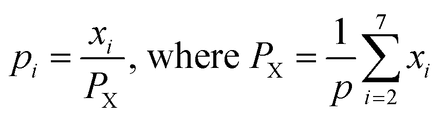
At t = 0, assuming x2 = x3 = 0; x7 = z, continuity equations are need to be satisfied and are expressed as:
Carbon balance:
| x1 + x5 + x6 = 1 | (7) |
Hydrogen balance:
| 2x4 + 4x6 = α + 2w | (8) |
Oxygen balance:
| x4 + 2x5 = 2y + β + w | (9) |
Steam balance:
| x4 = μx5 + w | (10) |
Now, the rate equations, based on the Langmuir–Hinshelwood mechanism, can be given as:
For Boudouard reaction (R1):
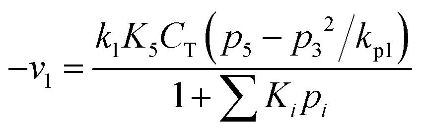 | (11) |
 | (12) |
Therefore, 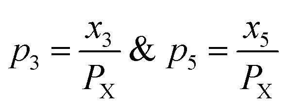 and using
 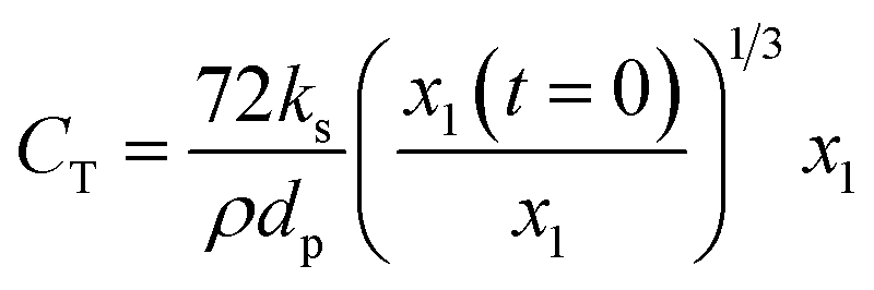 the Boudouard reaction (R1) eqn (11) can be rewritten as:
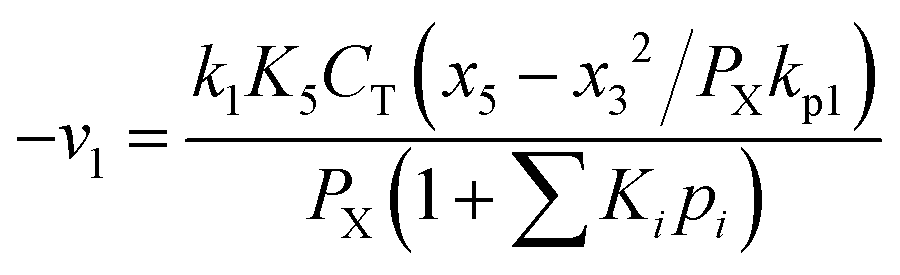
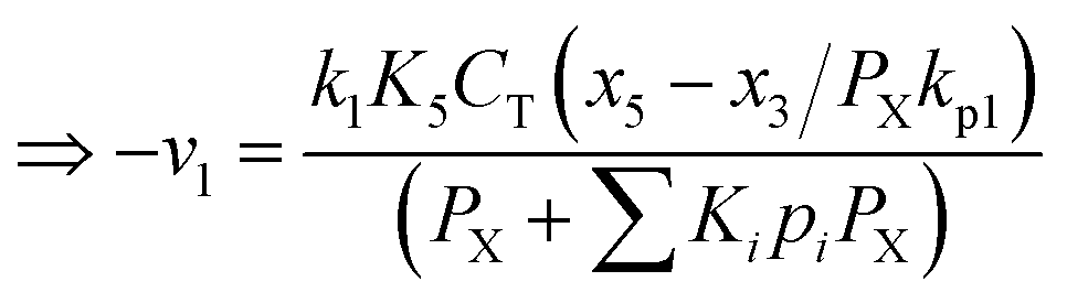
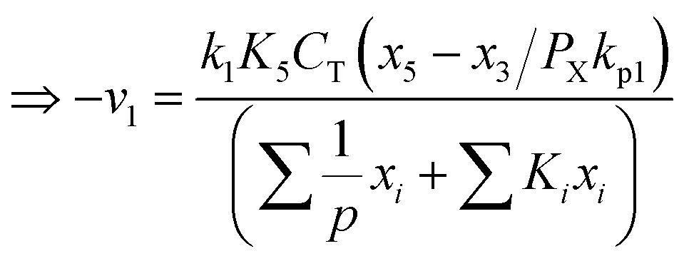
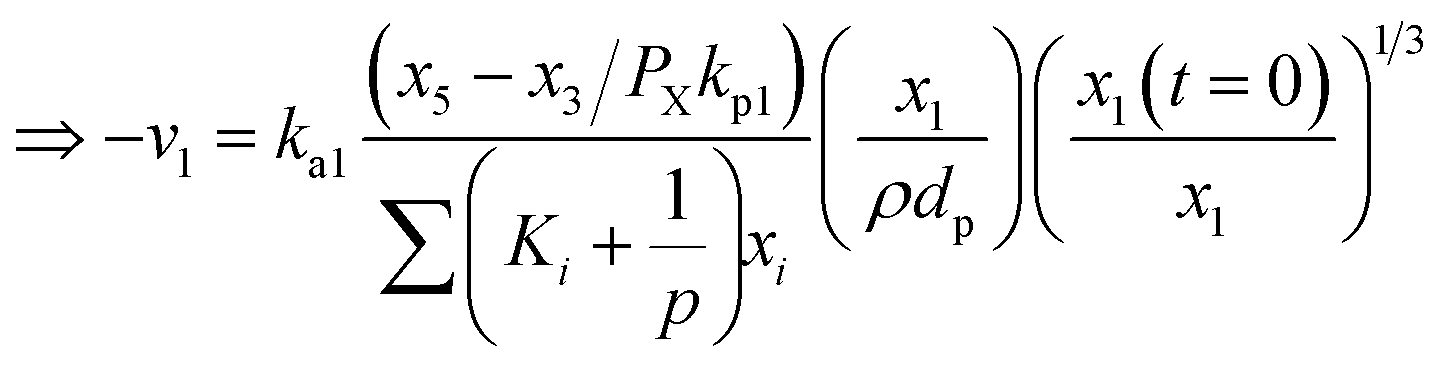 | (13) |
As a similar way like Boudouard reaction (R1), steam gasification (R2) is given as:
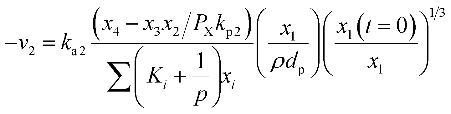 | (14) |
Hydrogen gasification (R3) can be expressed as:
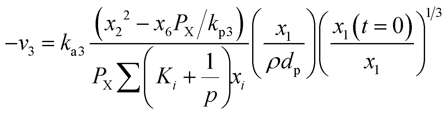 | (15) |
Methane–steam reforming (MSR) (R4) can be expressed as:
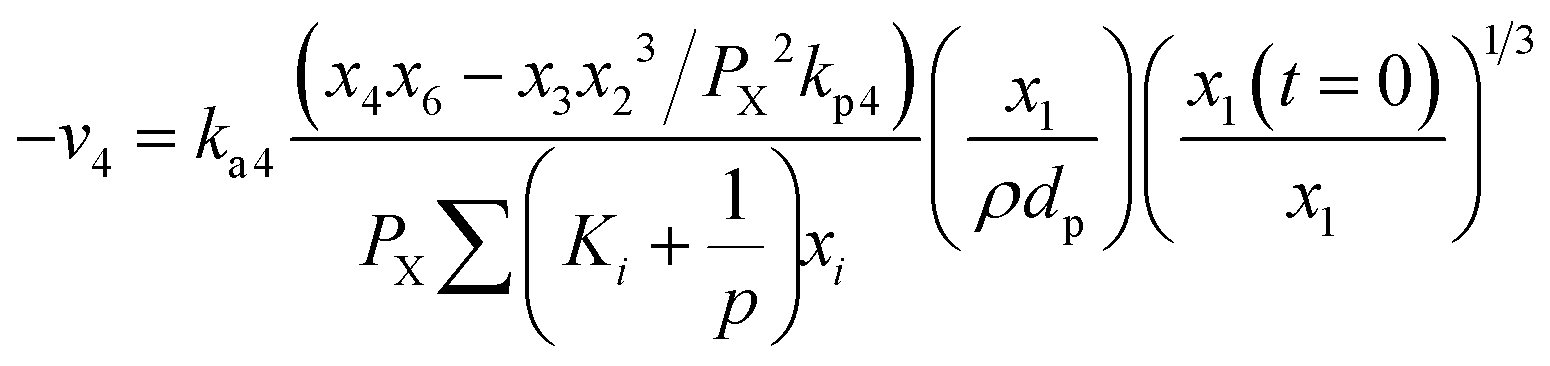 | (16) |
Water-gas shift (WGS) (R5) can be expressed as:
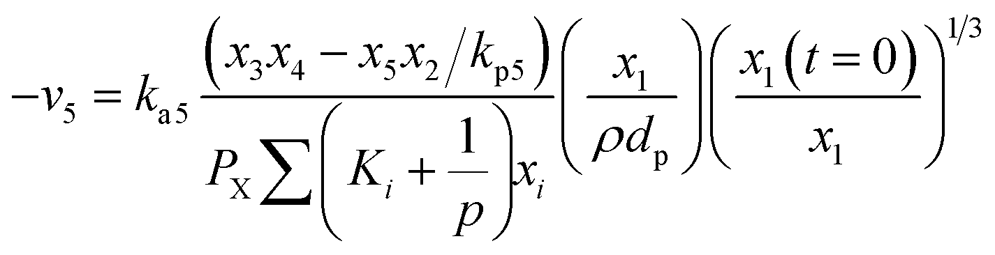 | (17) |
Now, using reactions (R1)–(R5) as given in eqn (13)–(17), differential equations can be formulated for solving the gas composition and carbon content. These are expressed as follows:
 | (18) |
 | (19) |
 | (20) |
 | (21) |
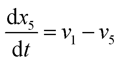 | (22) |
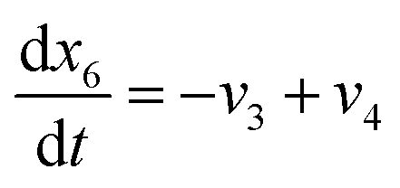 | (23) |
Eqn (18)–(23) are numerically solved by applying explicit methodology where starting guesses are taken from eqn (18)–(23). An in-house built FORTRAN code has been developed for solving the aforesaid equations to obtain the gas/carbon composition. Results obtain till the gasification reached a steady state condition where an error is kept fixed at 1% between two successive time steps.
2.3 Experimental set-up and procedure
The bubbling fluidized bed (BFB) gasifier setup at Process Engineering Research Laboratory of Indian Institute of Technology Roorkee20 was used in this study whose schematic PFD is shown in Fig. 1.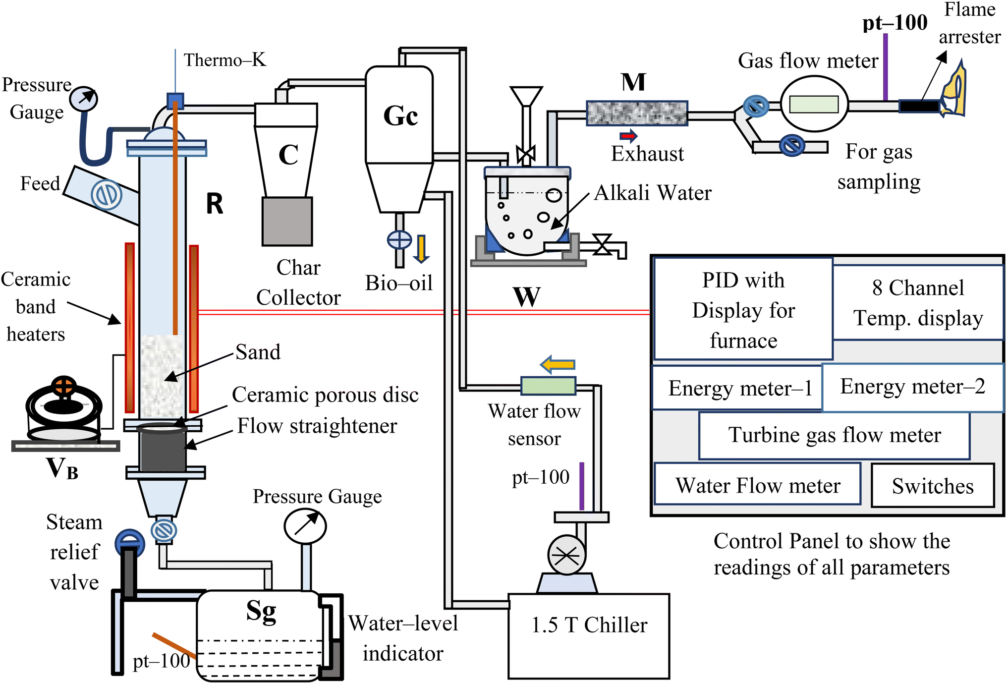 | ||
| Fig. 1 Schematic diagram of experimental setup. | ||
The reactor (R) (1.5 m tall × 0.102 m o.d.) made of stainless steel (SS-304), is electrically heated using ceramic band heaters (total height, 0.63 m) having kanthal-®A inner wire, which are controlled by a voltage barrier (VB) (set at 230 V). The “R” is covered with a highly insulated 2 to 3 cm thick layer of ceramic wool to prevent heat loss from the system to the surrounding. All the temperatures are dynamically sensed by the temperature thermocouples (TCs) (pt-100 and K-type (Nickel–Chromium)) and recorded in a temperature data logger at the control panel. These temperatures are regularly monitored and controlled using PID controllers (TC203 and TC344). The steam generator (Sg) having 15 L of water intake capacity, is designed for a maximum working pressure of 3 kg cm−2. The superheated steam (2 kg cm−2 at 140 ± 5 °C) followed by a preheating process, is used to fluidized the bed in the reactor (R). A bunch of Cu-tubes (length × diameter = 40 mm × 6 mm) are arranged vertically, gas-welded and used as a flow-straightener. A ceramic porous disc of 50 μm pore size is placed above the flow straightener. The EWS biomass is fed from the side-top section of the “R”, as shown in Fig. 1. The cyclone separator (C) is used to separate char and dust particles from the gasifier exhaust gas, collected in a char collection drum placed below the cyclone separator.
After that a gas cooler (Gc) (0.7 m tall × 0.20 m o.d.) is used to quench the gases/volatiles from “C”. The flow and temperature of cooling water inside “GC” are maintained by 0.25 HP centrifugal pump and water chiller unit, respectively. Then, the non-condensable/permanent gases (mainly CO, CH4, H2 and CO2) coming out from “GC” are passed through an alkali-water tank (W) so that tars and reaming dust can be separated from the gases. The clean and cool gases from “W” is sent to the moisture trap (M), having silica beads so that moisture from the gases can be removed. Then, the gaseous mixture is passed through a gas flow meter (E-TFM-11), which is used to quantify the total volume (in L) and volumetric flow rate (in L h−1) of gas produced during a particular run. The sample gas is collected in a Tedlar bag for analyzing it using a gas chromatogram analyzer (NEWCHROM 6700). The remaining gases are burned using a gas burner after these come out from the inline flame arrestor (MODEL: 872).
In order to construct different test cases, four input parameters at three levels are considered, as listed in Table 1.
| Parameters (units) | Low level (−1) | Mid-level (0) | High level (+1) |
|---|---|---|---|
| Equivalence ratio (ER, unitless) | 0 | 0.2 | 0.4 |
| Particle diameter (dp, μm) | 100 | 550 | 1000 |
| Reaction temperature (T, K) | 900 | 1050 | 1200 |
| Steam to biomass ratio (SBR, unitless) | 0.5 | 1.5 | 2.5 |
Based on experiment matrix given by design of experiment, simulations are performed and volumetric compositions of H2 and CO2 gases have been computed, as reported in Table 2.
| Runs | Parameters | Kinetic model | RSM-predicted | |||||||
|---|---|---|---|---|---|---|---|---|---|---|
| ER | dp (μm) | T (K) | SBR | H2 (vol%) | CO2 (vol%) | Utility | H2 (vol%) | CO2 (vol%) | Utility | |
| a Where, ER: equivalence ratio (mol mol−1), dp: Particle size (μm), T: gasification temperature (K), and SBR: steam to biomass ratio (mass/mass). | ||||||||||
| 1 | 0.2 | 550 | 1050 | 1.5 | 35.16 | 28.84 | 4.29 | 36.06 | 28.66 | 4.36 |
| 2 | 0 | 550 | 1050 | 1.5 | 46.77 | 17.69 | 7.59 | 41.55 | 20.25 | 6.03 |
| 3 | 0.4 | 100 | 900 | 0.5 | 27.08 | 39.10 | 1.51 | 29.62 | 39.22 | 2.06 |
| 4 | 0 | 100 | 900 | 0.5 | 46.45 | 19.21 | 7.39 | 46.27 | 18.73 | 7.38 |
| 5 | 0.4 | 1000 | 900 | 0.5 | 36.23 | 41.26 | 3.97 | 32.5 | 42.32 | 2.96 |
| 6 | 0 | 100 | 900 | 2.5 | 32.87 | 21.81 | 4.16 | 30.83 | 22.86 | 3.61 |
| 7 | 0.4 | 100 | 1200 | 0.5 | 38.44 | 33.78 | 4.82 | 38.29 | 33.11 | 4.78 |
| 8 | 0.4 | 100 | 1200 | 2.5 | 39.58 | 34.96 | 5.01 | 35.81 | 37.31 | 3.85 |
| 9 | 0 | 1000 | 1200 | 2.5 | 51.83 | 15.95 | 8.65 | 48.57 | 16.24 | 7.97 |
| 10 | 0.2 | 100 | 1050 | 1.5 | 31.35 | 30.29 | 3.21 | 32.91 | 28.85 | 3.71 |
| 11 | 0 | 1000 | 1200 | 0.5 | 52.19 | 14.37 | 8.88 | 54.92 | 13.76 | 9.4 |
| 12 | 0.4 | 1000 | 1200 | 0.5 | 38.45 | 33.79 | 4.82 | 39.76 | 33.14 | 5.23 |
| 13 | 0.2 | 1000 | 1050 | 1.5 | 39.54 | 27.34 | 5.41 | 37.68 | 28.84 | 4.89 |
| 14 | 0.4 | 100 | 900 | 2.5 | 23.25 | 42.57 | 0.03 | 21.32 | 42.76 | 0.34 |
| 15 | 0.2 | 550 | 1200 | 1.5 | 47.03 | 24.01 | 7.14 | 45.22 | 24.39 | 6.85 |
| 16 | 0.2 | 550 | 1050 | 2.5 | 27.85 | 32.24 | 2.07 | 32.54 | 29.49 | 3.44 |
| 17 | 0.4 | 550 | 1050 | 1.5 | 24.29 | 42.38 | 0.43 | 29.21 | 39.89 | 1.96 |
| 18 | 0.4 | 1000 | 1200 | 2.5 | 39.57 | 34.97 | 5.01 | 40.55 | 35.02 | 5.17 |
| 19 | 0 | 100 | 1200 | 2.5 | 37.39 | 20.83 | 5.36 | 41.92 | 19.35 | 6.51 |
| 20 | 0.2 | 550 | 1050 | 0.5 | 44.86 | 23.67 | 6.75 | 39.87 | 26.48 | 5.35 |
| 21 | 0 | 100 | 1200 | 0.5 | 52.10 | 14.21 | 8.89 | 51.53 | 14.56 | 8.82 |
| 22 | 0.4 | 1000 | 900 | 2.5 | 27.62 | 43.48 | 1.51 | 27.46 | 43.53 | 1.44 |
| 23 | 0 | 1000 | 900 | 2.5 | 37.94 | 22.55 | 5.36 | 38.89 | 22.8 | 5.53 |
| 24 | 0.2 | 550 | 900 | 1.5 | 34.54 | 31.04 | 4.02 | 36.05 | 30.73 | 4.27 |
| 25 | 0 | 1000 | 900 | 0.5 | 48.02 | 22.93 | 7.39 | 51.07 | 20.99 | 8.42 |
2.4 Response surface methodology
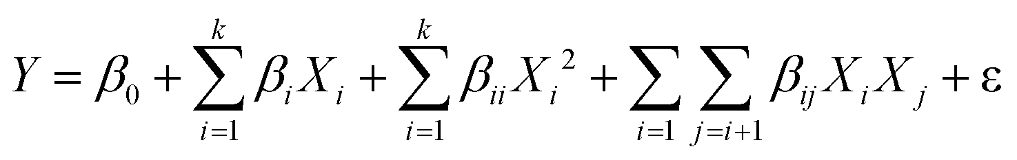
The central composite design (CCD) technique is employed to conduct the optimization analysis. A quadratic model, as a function of independent input parameters, is opted for predicting maximum H2 (vol%) and minimum CO2 (vol%), expressed in eqn (24):21
 | (24) |
2.5 Utility concept
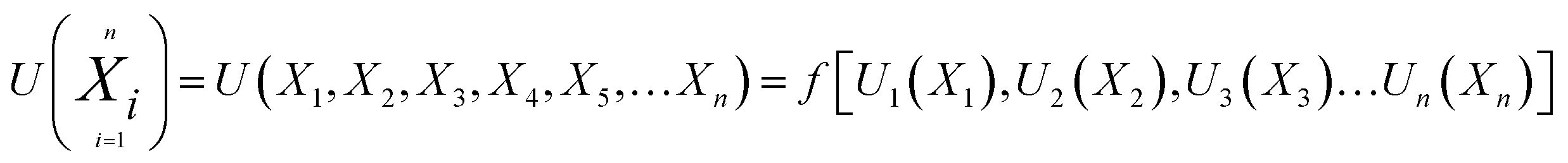
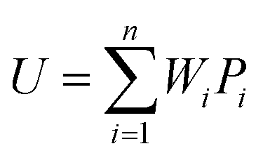
Any physical problem, it is important to get the maximum performance of the system and that is why optimization of multi-objective function is necessary to be analyzed. In that context, utility concept is important where different objective functions are clubbed together into a single objective function and depending upon their respective usage, maximum/minimum utilization of the system can be evaluated. The overall utility of the EWS gasification is computed as the total sum of all the performance utility characteristics i.e., enriching H2 concentration and diminishing CO2 gas emission. “U” = overall utility function [f(Xi)], refers the effective quantity of ith performance characteristics, is given by as below:22
 | (25) |
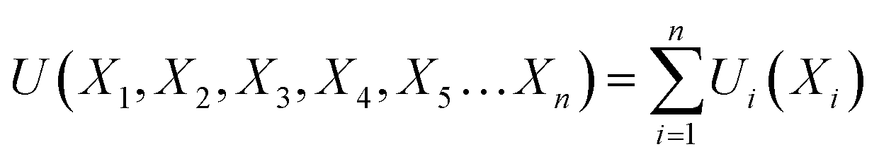
The overall utility is calculated as the summation of individual utility and is given as:
 | (26) |
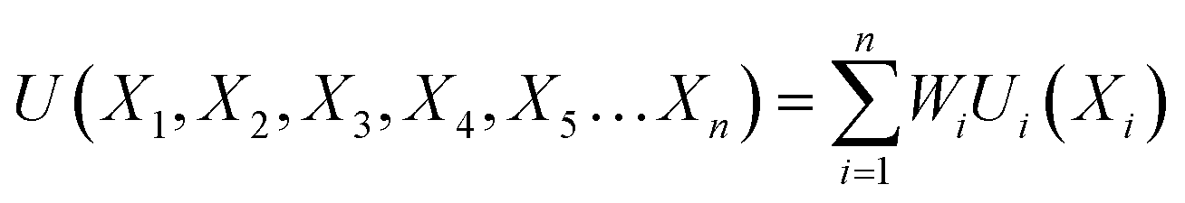
Based on the requirement of the system under consideration (like gasification in this study) priorities are given to the performance characteristics and accordingly appropriate weights are assigned. Finally, the overall utility can be rewritten as:
 | (27) |
 | (28) |
For finding the utility value for a number of performances generally involves a preference scale and weightages are assigned. For this purpose, a logarithmic scale is considered and a preference number is calculated between 0 to 9 where 0 = the least acceptable quality and 9 = the finest quality. This can be expressed as:23
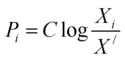 | (29) |
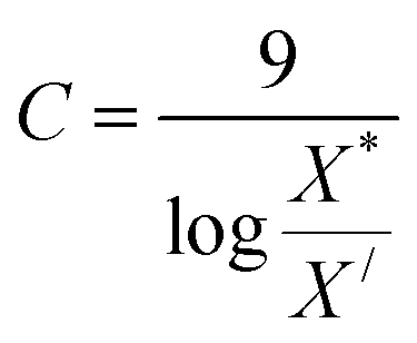
For finding C value preference number is set as 9 and Xi = X* where X* = optimum value. This can be represented as:
 | (30) |
 | (31) |
3. Results and discussion
3.1 Validation
Study on EWS gasification for optimum operating condition of the gasifier has been performed involving chemical kinetic modeling. The kinetic model includes various gasification reactions including gas shift reaction in the form of differential equations. The equations need to be solved in order to obtain the composition of syngas production. To obtain results, an in-house built FORTRAN code has been developed satisfying the initial conditions and utilizing explicit method. As the reactions are time dependent, so iterations are performed until steady state condition is arrived. It is important to perform validation work before proceed for different case studies. Validation has been performed for different compositions of syngas production with different feed material and results generated by present code are compared with that of the available literature. In addition, experiments are performed in a lab scale setup using EWS biomass and the syngas compositions are compared with the results obtained by the present FORTRAN code using chemical kinetic model. All these validation parts are illustrated in Fig. 2 along with the RMSE value, calculated as: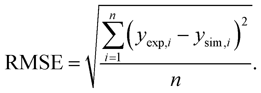 It can be seen from the figure that the present kinetic model predicts syngas composition closer to the experimental one and the RMSE value lies well within the acceptable range. This validation encourages for conducting other case studies required for the analysis.
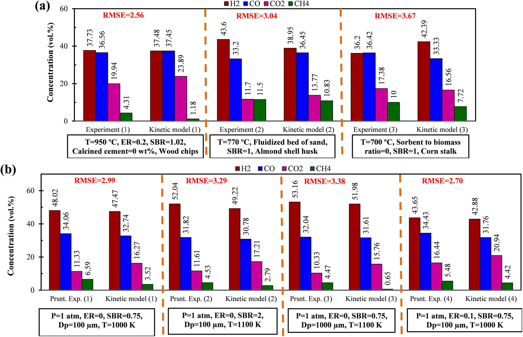 | ||
| Fig. 2 Comparison of syngas composition between present kinetic model with (a) experiment-1,24 experiment-2,25 experiment-3 (ref. 26) (b) present experiments using EWS biomass. | ||
3.2 Maximizing H2 production and minimizing CO2 emission
In biomass gasification it is common to produce hydrogen rich syngas because of having higher heating value of hydrogen gas. In this study EWS biomass is used as a feedstock material and involving chemical kinetic modeling many experimental cases are planned for finding suitable condition for maximum H2 production. But such process is a time taking, and inefficient. Hence, optimization tool is important to minimize this effort. Here, response surface methodology (RSM) is employed as optimization tool with two different single objective functions i.e. (i) finding the best condition for maximum H2 gas production (ii) minimizing CO2 gas production. There are four input parameters such as equivalence ratio (ER), particle size (dp), gasification temperature (T), steam to biomass ratio (SBR) and two output parameters i.e., vol% of H2 and CO2 gas and using these parameters RSM optimization will be performed. For analyzing only 25 numbers of experimental cases/runs are required, given by design of experiments, as tabulated in Table 2.Table 3 represents the analysis of variance (ANOVA) table for both the objective functions. For first objective function i.e. maximizing H2 gas, one can see in Table 3 that lower p-values (<0.05) of input parameters (such as ER, dp, T, and SBR) indicate that all these parameters are significant for H2 production but parameters like ER followed by T are the most influential one. However, p-values for square & two-way interaction parameters are found “(>0.05)” and thus insignificant for the objective function. A quadratic model is developed for H2 gas which is a function of all input parameters is expressed in eqn (32). The ANOVA table also gives that the p-value for the quadratic model is 0.0049 (<0.05) which confirms the robustness of the developed model. For the second objective function i.e., minimizing CO2 gas production, Table 3 shows that except dp all other parameters are significant. Because of the smallest p-value, ER is the most influential parameter followed by T and SBR. The quadratic model is given in eqn (33) and its lower p-value (<0.0001) certifies the authenticity of the model.
| Response | H2 (vol%) | CO2 (vol%) | ||||
|---|---|---|---|---|---|---|
| Source | Coefficient | p-value | Remark | Coefficient | p-value | Remark |
| Model | 0.0049 | Significant | <0.0001 | Significant | ||
| Intercept (β0) | 36.06 | 28.66 | ||||
| ER | −6.17 | 0.0002 | Significant | 9.82 | <0.0001 | Significant |
| dp | 2.38 | 0.0496 | Significant | −0.01 | 0.9910 | Insignificant |
| T | 4.59 | 0.0016 | Significant | −3.17 | 0.0001 | Significant |
| SBR | −3.66 | 0.0064 | Significant | 1.50 | 0.0159 | Significant |
| ER2 | −0.68 | 0.8157 | Insignificant | 1.41 | 0.3299 | Insignificant |
| dp2 | −0.76 | 0.7933 | Insignificant | 0.19 | 0.8949 | Insignificant |
| T2 | 4.57 | 0.1381 | Insignificant | −1.10 | 0.4431 | Insignificant |
| SBR2 | 0.14 | 0.9610 | Insignificant | −0.67 | 0.6359 | Insignificant |
| ER × dp | −0.48 | 0.6818 | Insignificant | 0.21 | 0.7121 | Insignificant |
| ER × T | 0.85 | 0.4686 | Insignificant | −0.49 | 0.3976 | Insignificant |
| ER × SBR | 1.78 | 0.1459 | Insignificant | −0.15 | 0.7930 | Insignificant |
| dp × T | −0.35 | 0.7622 | Insignificant | −0.76 | 0.1942 | Insignificant |
| dp × SBR | 0.82 | 0.4873 | Insignificant | −0.58 | 0.3167 | Insignificant |
| T × SBR | 1.46 | 0.2271 | Insignificant | 0.17 | 0.7681 | Insignificant |
| LOF | 5.56 | Insignificant | 29.35 | Insignificant | ||
| Regression analysis | R2 = 0.8863, adj. R2 = 0.7270, adeq precision = 9.58, std dev. = 4.53, mean = 38.42, CV% = 11.78, PRESS = 1317.19 | R2 = 0.9762, adj. R2 = 0.9430, adeq precision = 17.49, std dev. = 2.20, mean = 28.53, CV% = 7.71, PRESS = 283.66 | ||||
The centre composite design (CCD) technique recommends 25 number of experiments which includes 16 factorial, 8 axial, and 1 center points experiments of input parameters (ER, dp, T, SBR). These suggested runs are numerically performed by adopting the developed FORTRAN code involving chemical kinetic modeling. The obtained value of H2 and CO2 gas compositions are used in the design matrix, suggested by design expert software (Design-Expert v22.0), to perform further investigations such as analysis of suggested model, optimization, and graphical interpretation. Finally, a mathematical model (2nd-order) is obtained for maximum volumetric composition of H2 and CO2 as shown in eqn (32) and (33), respectively, in the coded factors units.
| H2 (vol%) = 36.06 − 6.17 × ER + 2.38 × dp + 4.59 × T − 3.66 × SBR − 0.68 × ER2 − 0.76 × dp2 + 4.57 × T2 + 0.14 × SBR2 − 0.48 × ER × dp + 0.85 × ER × T + 1.78 × ER × SBR − 0.35 × dp × T + 0.82 × dp × SBR + 1.46 × T × SBR | (32) |
| CO2 (vol%) = 28.66 + 9.82 × ER − 6.0 × 10⁻³ × dp − 3.17 × T + 1.50 × SBR + 1.41 × ER2 + 0.19 × dp2 − 1.10 × T2 − 0.67 × SBR2 + 0.21 × ER × dp − 0.49 × ER × T − 0.15 × ER × SBR − 0.76 × dp × T − 0.58 × dp × SBR + 0.17 × T × SBR | (33) |
Fig. 3(a)–(c) shows 3-D surface plots for H2 production for a variation of any two operating parameters keeping other parameters fixed at their center points. The plots are useful to find out a small area, defined by the reduced ranges of operating parameters, in which the maxima of H2 production lies. The importance of any input parameter on output parameter is determined by the slope of the curve, Fig. 3(a)–(c). It is observed that all the input parameters developed a steep slope for H2 production representing the significant effect of all these parameters. Fig. 3(a) depicts the combined effects of ER and dp on the H2 production. It shows that when ER is increased from 0 to 0.4 there is a rapid decrease in H2 production. When dp increases from 100 to 1000 μm, H2 production rises slowly. The variation of H2 production with T and dp is given in Fig. 3(b). It can be seen that maximum H2 production is found at 1200 K temperature and 1000 μm particle diameter. The effect of SBR and T on the H2 production is shown in Fig. 3(c), it reveals that at SBR = 0.5 to 2.5 range H2 production diminishes. Therefore, the optimum setting for maximum H2 production, the quadratic model gives an accurate setting i.e., ER = 0, dp = 950 μm, T = 1170 K, and SBR = 0.5 predicted by central composite design at which maximum 51.72 vol% H2 production is achieved. Fig. 3(d)–(f) shows 3-D surface plots for CO2 minimization while varying two input parameters by taking other parameters fixed at their centre point values. By varying dp from 100 to 1000 μm there is hardly any change in CO2 concentration; however, CO2 concentration decreases when ER decreases from 0.4 to 0, as shown in Fig. 3(d). Fig. 3(e) represents the variation of CO2 with T and dp. The CO2 emission reduces with rising T values whereas the reduction is comparatively less with dropping in dp value. Fig. 3(f) shows that by augmenting gasification temperature and decreasing SBR diminishes CO2 gas production. By analyzing Fig. 3(d)–(f) for obtaining the second objective function i.e., CO2 minimization, the model predicts the optimum setting as ER = 0, dp = 794 μm, T = 1150 K, and SBR = 0.5 where the CO2 gas composition is predicted as 15.51 vol%.
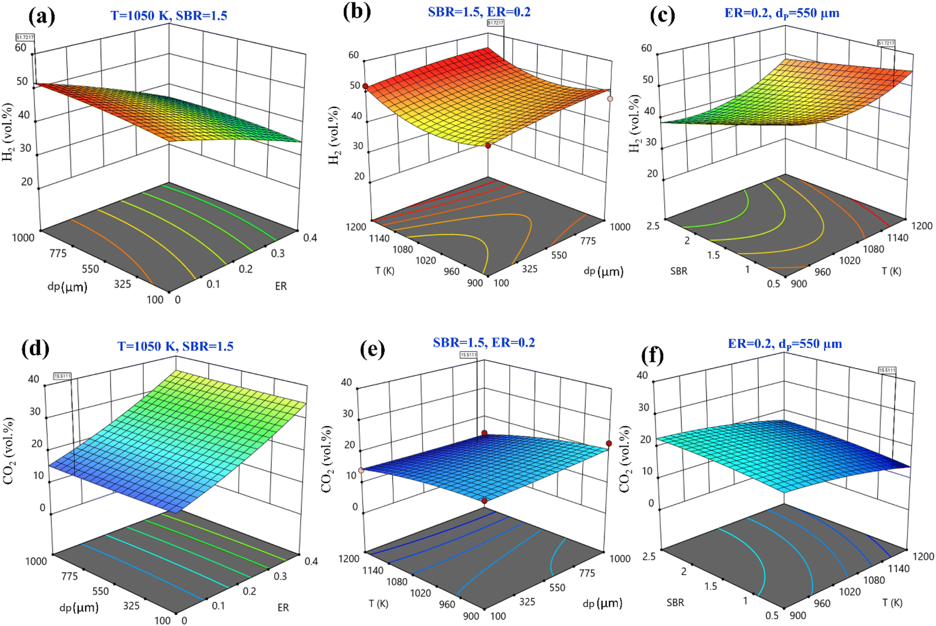 | ||
| Fig. 3 Three-dimensional surface plots for (a–c) H2 maximization and (d–f) CO2 minimization. | ||
Instead of analyzing three different 3-D surface plots, one can visualize the same by seeing a single figure like perturbation plot, as shown in Fig. 4. Such figure is important from the subject point of view as it describes the impact of each input parameter on the output parameter. The path traced by an individual parameter denotes its sensitivity or insensitivity on the output parameter like higher the slope more the sensitive parameter whereas less slope or flat line shows its insensitivity. The impact of varying parameters such as ER, dp, T, SBR on H2-rich syngas production using EWS biomass is shown in Fig. 4(a). It is noticed that parameter ‘ER’ has attained the highest slope (from 0 to 0.4) and hence it is the most influential parameter. The plausible reason is that change in ER-value from 0.4 to 0 reduces the oxygen supply in the gasifier which in-turn suppresses the emission of CO2 gases resulting in the increase in H2 gas composition. Parameter ‘T’ has attained the second highest slope in the range 1050 to 1200 K. With rise in temperature the volumetric concentration of H2 rapidly increases because of the sudden jump of the equilibrium constant values of Boudouard (R1), steam gasification (R2), and methane-steam reforming (R4) reactions. Parameter ‘SBR’ gives the third highest slope where H2 production drops with supplying excessive steam that starts the reverse-water-gas shift (rev-WGS) reaction. The path traced by parameter ‘dp’ approaches closely to a flat line and hence it is the least significant factor for H2-rich syngas production. EWS biomass particle size stimulates the residence time but the present analysis considers steady state condition to obtain the gas compositions and that is why parameter ‘dp’ is comparatively less affective for maximum H2 gas production. Fig. 4(b) depicts the effect of input parameters on CO2 gas production. By observing this figure, one can easily identify parameter ‘ER’ as the most dominant factor in CO2 gas reduction. The argument is already discussed above emphasizing that lower oxygen supply at small value of ER leads to partial oxidation of EWS biomass followed by minimum CO2 generation. Secondly, referring to Boudouard reaction (R1), increase in temperature reduces CO2 concentration as carbon reacts with CO2 to produce CO gas and that is why parameter ‘T’ attains the second highest slope. It is also to be noticed that SBR-curve followed by dp-curve has negligible slope and hence they are relatively less significant parameters compared to others.
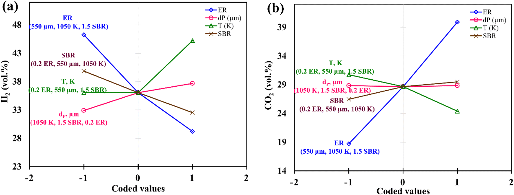 | ||
| Fig. 4 Perturbation plot for (a) H2 maximization (b) CO2 minimization. | ||
3.3 Utility concept
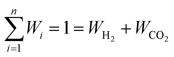
In this study, utility concept is employed to combine two objective functions, i.e. (i) H2 maximization and (ii) CO2 minimization, into a single objective function by applying appropriately weightage to the respective objective functions depending upon the usage of the gasification process. Usually, gasification focusses on production of high heating value gases like H2-gas without affecting the surrounding environmental condition like low CO2 production. Hence, more weightage is given to the first objective function and less weightage to the second objective function. The present analysis considers weightage as 80:20 ratio for framing the utility function as the maximization case.
Table 4 represents the ANOVA table for utility function. It can be seen from the table that except particle diameter of EWS biomass, all the three parameters have significant effect on utility function in the order like ER > T > SBR. The interaction between two parameters and square terms are found insignificant for the utility model. RSM generates a quadratic model for utility function involving all input parameters (i.e., dp, ER, T, SBR), as given in eqn (34).
| U = 4.36 − 2.03 × ER + 0.59 × dp + 1.29 × T − 0.96 × SBR − 0.36 × ER2 − 0.063 × dp2 + 1.21 × T2 + 0.037 × SBR2 − 0.035 × ER × dp + 0.32 × ER × T + 0.34 × ER × SBR − 0.12 × dp × T + 0.22 × dp × SBR + 0.37 × T × SBR | (34) |
| Source | Coefficient | p-value | Remark |
|---|---|---|---|
| a For utility (U) function, the model equation in coded factors units. | |||
| Model | 0.0030 | Significant | |
| β0 | 4.36 | ||
| ER | −2.03 | <0.0001 | Significant |
| dp | 0.59 | 0.0738 | Insignificant |
| T | 1.29 | 0.0014 | Significant |
| SBR | −0.96 | 0.0089 | Significant |
| ER2 | −0.36 | 0.6533 | Insignificant |
| dp2 | −0.06 | 0.9378 | Insignificant |
| T2 | 1.21 | 0.1563 | Insignificant |
| SBR2 | 0.04 | 0.9633 | Insignificant |
| ER × dp | −0.03 | 0.9136 | Insignificant |
| ER × T | 0.32 | 0.3290 | Insignificant |
| ER × SBR | 0.34 | 0.2998 | Insignificant |
| dp × T | −0.12 | 0.7200 | Insignificant |
| dp × SBR | 0.22 | 0.5007 | Insignificant |
| T × SBR | 0.37 | 0.2712 | Insignificant |
| LOF | 6.30 | Insignificant | |
| Regression analysis | R2 = 0.8982, adj. R2 = 0.7555, adeq precision = 10.02, std dev. = 1.26, mean = 4.95, CV% = 25.38, PRESS = 98.32 | ||
Fig. 5 shows the three-dimensional surface plot for utility. Fig. 5(a) illustrates that increase in utility function is obtained at higher EWS particle size and lower ER value. Keeping the remaining parameters constant at their mid-values, both higher temperature and particle size maximizes the utility value, as shown in Fig. 5(b), whereas it is also maximum at small SBR and temperature value, as shown in Fig. 5(c). By analyzing Fig. 5(a)–(c) and satisfying the objective function i.e., utility maximization, the RSM predicts the optimum setting as ER = 0, dp = 840 μm, T = 1150 K, and SBR = 0.5 where the H2 and CO2 gas compositions are given as 51.54 vol% and 15.52 vol%, respectively.
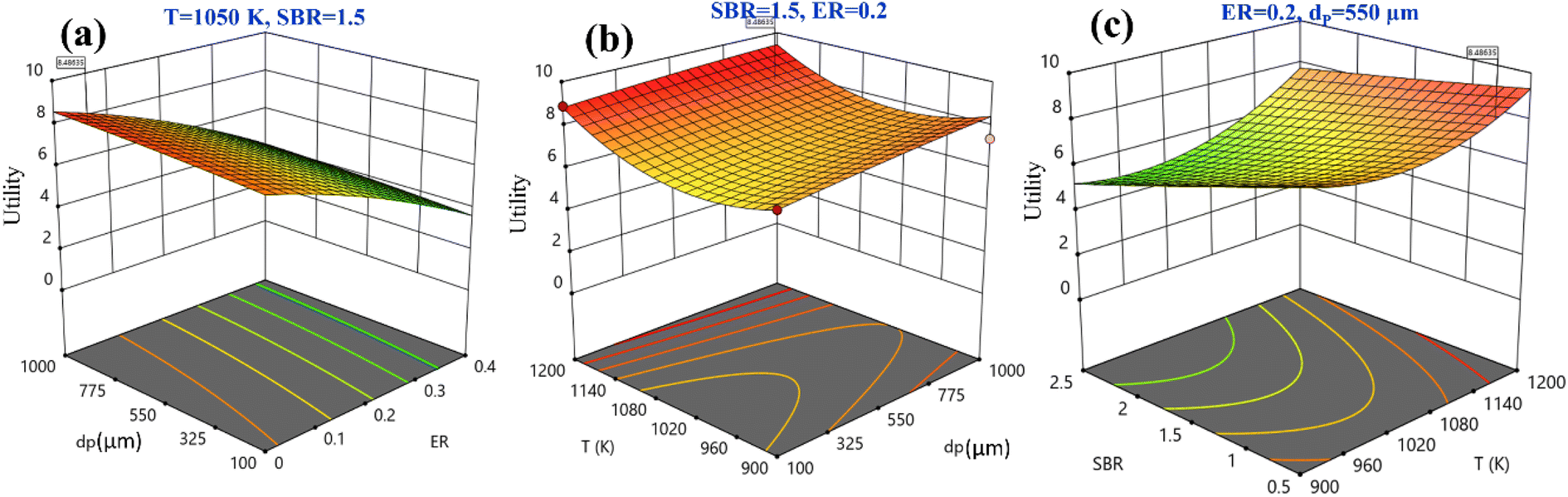 | ||
| Fig. 5 Three-dimensional surface plots for utility maximization. | ||
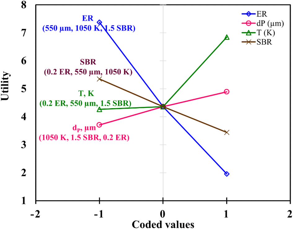
Fig. 6 demonstrates the effect of each input parameters on utility function. It can be observed that for maximizing the utility function, parameter ‘ER’ has the highest contribution followed by parameter ‘T’, ‘SBR’, and ‘dp’. The trend of each parameter for the utility function is similar to that of the first objective function i.e., H2 gas maximization and the reason is already discussed in the earlier section (Fig. 4(a)). This trend is quite obvious because while forming utility function more weightage (80%) is given to H2 gas composition and less weightage (20%) to CO2. It is found that for single objective function H2 maximization case gives 51.72 & 15.57 vol% of H2 & CO2 concentrations and CO2 minimization case gives 51.45 & 15.51 vol% of H2 & CO2 gas compositions whereas utility gives 51.54 vol% and 15.52 vol% of H2 and CO2 gas compositions. After critically analyzed the scenario, the authors noticed that for the maximum utilization of gasification of EWS biowaste there is a reduction in H2 gas production in the expense of more CO2 emission. In order to validate the syngas compositions, at optimum condition given by utility concept, the results obtained by kinetic model are compared with the experimental one and quadratic model, as shown in Fig. 7. The figure shows that syngas compositions obtained by different models are found close (std. deviation: σ ≤ 2.245 for H2 and σ ≤ 2.885 for CO2 gas compositions) to the experimental results which confirms the reliability or robustness of the models.
 | ||
| Fig. 6 Perturbation plot for utility maximization. | ||
 | ||
| Fig. 7 Comparison of H2 and CO2 gas compositions between different models and experiment at optimum condition (ER = 0, dp = 840 μm, T = 1150 K, SBR = 0.50). | ||
3.4 Techno-economic analysis
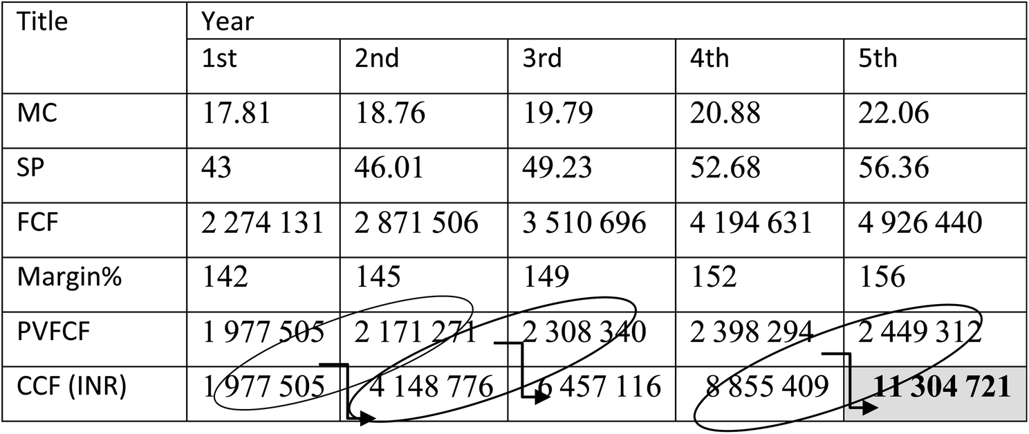
The present study focuses on maximum utilization of biomass gasification process for H2 rich syngas production with minimum CO2 emission through chemical kinetic modeling. On the other hand, global energy market demands continuous rise in green energy production (e.g., H2) in order to limit the dependency on fossil fuel and preventing the greenhouse gases emission. In this regard, it is important to linkup the current analysis with the industrial level like finding the large-scale usage of EWS biomass and checking the feasibility of H2 production in bulk amount. Apart from the technical part, cost analysis is an important tool for deciding the usage of EWS biomass in industrial plant. Such analysis is called techno-economic analysis where both technological and cost analysis/plant economics are simultaneously investigated.For economic analysis of EWS biomass, an industrial level “down draft 20 kW h−1 biomass pyrolysis gasifier” setup is considered. This analysis is conducted for a pilot plant, having a capacity of 500 m3 per day of syngas production. Economic analysis involves computing the following items such as (i) fixed cost [FC] (ii) operating cost [OC] (iii) raw material cost [CRM] (iv) manufacturing cost [MC] (v) selling price [SP] (vi) total annual cost [TAC] (vii) annual cost of capital recovery [ACCR] (viii) payback period [PP]. Fixed cost primarily involves equipment/machinery cost and its related cost such as installation, delivery cost, instrumentation-control-piping-electrical arrangement cost, building cost, courtyard improvement cost, contingency and contractor fee etc.27 The gasifier equipment (for 500 m3 per day syngas production, waste processing capacity of 2000 kg per day) cost is taken from ‘Sakthi Veera Green Energy Pvt. Ltd, Chennai [India]’ manufacturing company. For computation of the plant operating cost, following data are collected from market survey and are shown in Table 5. Based on the optimum condition, obtained from the utility concept, manufacturing cost (INR per kg) and plant payback period (year) are estimated.
| Title | Specifications |
|---|---|
| Production capacity | 500 m3 per day of syngas production |
| Service life | 20 years |
| Electricity consumption | 20 kW h−1 |
| Equipment operating time | 20 h per day |
| Equipment cost | 24 lakhs |
| No of shift/day | 3 |
| Working days | 300 days per year |
| Cost of raw material | 2 INR per kg |
| Wage of one labour | 500 INR/8 h |
| Cost of electricity | 5.5 INR per unit |
| Labours per shift | 5 nos |
| No. of trucks | 2 |
| Cost per truck | 80000 INR per month |
| Syngas yield | 693 g syngas per kg biomass |
| Inflation/depreciation rate | 7% annually |
The crucial part of techno-economic study is to obtain the plant payback period i.e., in how many years the invested capital will be recovered. The entire computation is elaborately discussed in seven consecutive steps as given below:
Step I: fixed cost [FC]:
Fixed cost comprises of equipment cost [E]; direct cost [DC] i.e., insulation [8.5% of E], purchased equipment delivery [E × 10%], installation [E × 40%], instrumentation and control [E × 18%], piping [E × 60%], electrical systems [E × 12.5%], buildings [E × 15%], yard improvements [E × 15%], service facilities [E × 55%], land [E × 6%]; repair & maintenance cost [E × 4%]; indirect cost [IC] i.e., engineering and supervision [(DC + E) × 8%], construction expenses [(DC + E) × 10%]; contractor's fee [(DC + IC) × 6%], and contingency [(DC + IC) × 8%].
Therefore, FC = E + DC + IC + Contr. fee + conti. = 10736832 INR.
Step II: annual cost of capital recovery [ACCR]:
ACCR is computed using the mathematical expression given as:
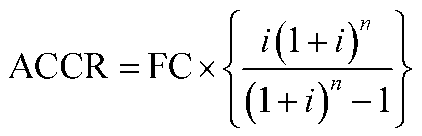
So, ACCR = 1715332.07 INR per year (taking i = 15% and n = 20 years).
Step III: operating cost [OC]:
The operating cost consists of cost of raw material, labor, transportation, and electricity. As per data provided in Table 5, the operating cost of envisaged gasification plant is calculated as:
OC = cost of (raw material + labor + transportation cost + electricity) = (1200000 + 2250000 + 1578080 + 660000) = 5688080 INR per year.
Step IV: manufacturing cost [MC]:
For syngas production,
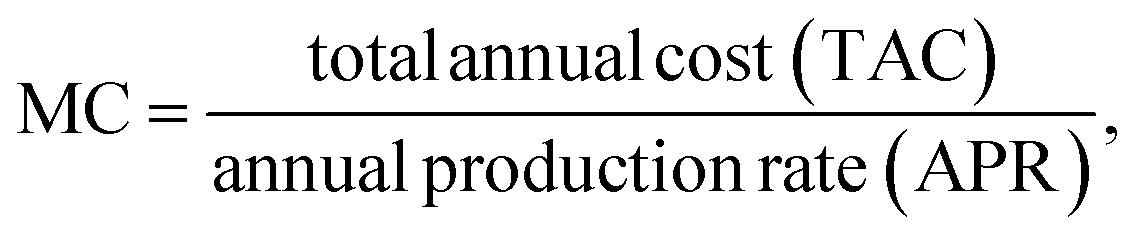
Here, 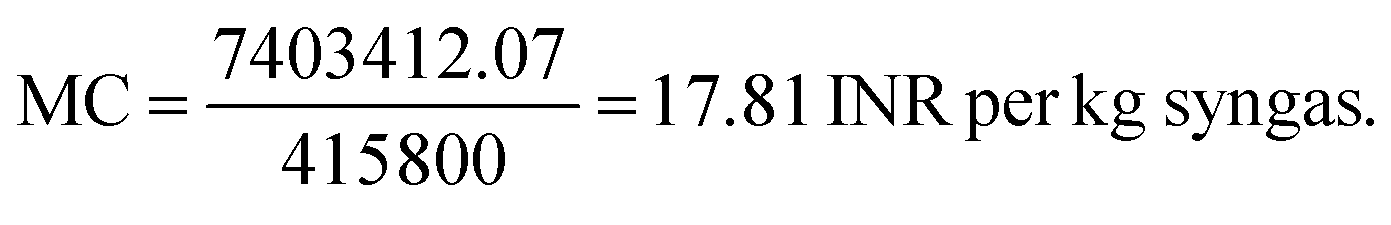
Step V: depreciation cost (D) using diminishing value method:
Salvage value (SV) after n years = FC × (1 − annual depreciation)n. Here, D = 411092.43 INR per year where 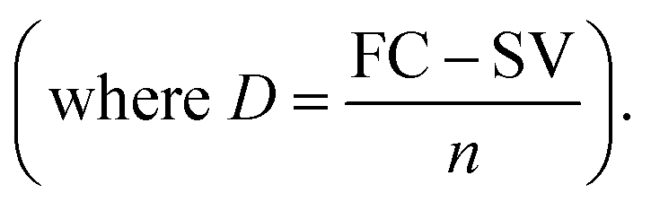
Step VI: profit and cash flow:
Net profit = GPAD − income tax on GPAD, where, GPAD = gross profit before depreciation = [(SP of syngas − MC) × APR] − TAC. The SP of syngas is set in such a way that GPAD will be a positive value. Considering SP = 43 INR per kg, income tax = 30%, the net profit = 1863038.41 INR per year. Future cash flow (FCF) = net profit + D = 2274130 INR per year. Present value of future cash flow (PVFCF) for 
Step VII: payback period:
In order to analyze the economic feasibility for setting up a biomass gasification plant, for H2-rich syngas production using eucalyptus wood sawdust, it is important to find out the payback period of the plant so that required profit margin can be targeted in the succeeding years. In the present analysis for a 20 years lifespan gasification plant considering all the major economic factors, the payback period is estimated as 4.8 (∼5) years, shown in Table 6.
| a Abbreviations: MC: manufacturing cost; SP: selling price; FCF: future cash flow; PVFCF: present value of future cash flow; CCF: cumulative cash flow. |
|---|
 |
4. Conclusions
In this study, RSM-utility concept based optimization has been implemented in a gasification process considering eucalyptus wood biomass where a chemical kinetic model is used to compute the syngas composition. The modified kinetic model, involving water gas shift reaction, is validated with lab scale experiments, available literature and the RMSE value lies well within the acceptable range (2.56 ≤ RMSE ≤ 3.67). In order to find out the optimal setting for maximum H2 gas production and reducing CO2 gas emission in air–steam gasification process, this research work is necessary. Results showed that the maximum H2 is obtained at ER = 0, dp = 950 μm, T = 1170 K, and SBR = 0.5 with 51.75 vol% production whereas minimum CO2 is obtained at ER = 0, dp = 794 μm, T = 1150 K, and SBR = 0.5 with 14.65 vol% production. Using utility concept (80% H2:20% CO2), the optimum H2 is computed as 51.69 vol% (0.11%↓) with a penalty of higher CO2 production found as 14.70 vol% (0.34%↑). ANOVA reveals that ER is the most influential parameter followed by T, SBR and dp. For predicting H2 and CO2 gas composition, RSM proposes two quadratic models comprises of four input parameters. In order to understand the feasibility of using EWS biomass at an industrial scale (500 m3 per day of syngas production capacity) for H2 rich syngas production, a detailed technoeconomic study has been reported. The analysis indicates that for a 20 years life span gasification plant, the payback period is 4.8 (∼5) years where fixing the selling price of H2 rich syngas at 43 INR per kg a minimum 142% profit margin can be availed. The complete study gives a clear direction that if H2 can be produced at optimum condition using EWS biomass, it could be an attractive option as energy source in the market.Conflicts of interest
There are no conflicts to declare.Acknowledgements
This research work is dedicated to our beloved professor B. Mohanty (Late), IIT Roorkee. His continuous effort, inspiration, guidance motivates the authors to produce quality work. Professor Mohanty's conceptualization helped to frame this research article.References
- Z. R. Gajera, K. Verma, S. P. Tekade and A. N. Sawarkar, Bioresour. Technol. Rep., 2020, 11, 100479 CrossRef.
- M. Rashidi and A. Tavasoli, J. Supercrit. Fluids, 2015, 98, 111–118 CrossRef CAS.
- W. Song, C. Deng and S. Guo, ACS Omega, 2021, 6, 11192–11198 CrossRef CAS PubMed.
- W. M. Champion, C. D. Cooper, K. R. Mackie and P. Cairney, J. Air Waste Manage. Assoc., 2014, 64, 160–174 CrossRef CAS PubMed.
- Y. Cao, Y. Bai and J. Du, Sci. Total Environ., 2021, 753, 141690 CrossRef CAS PubMed.
- L. P. R. Pala, Q. Wang, G. Kolb and V. Hessel, Renewable Energy, 2017, 101, 484–492 CrossRef CAS.
- M. B. Nikoo and N. Mahinpey, Biomass Bioenergy, 2008, 32, 1245–1254 CrossRef CAS.
- M. Shahbaz, S. Yusup, A. Inayat, M. Ammar, D. O. Patrick, A. Pratama and S. R. Naqvi, Energy Fuels, 2017, 31, 12350–12357 CrossRef CAS.
- J. A. Okolie, E. I. Epelle, S. Nanda, D. Castello, A. K. Dalai and J. A. Kozinski, J. Supercrit. Fluids, 2021, 173, 105199 CrossRef CAS.
- V. Silva and A. Rouboa, Energy Convers. Manage., 2015, 99, 28–40 CrossRef CAS.
- R. Bakari, T. Kivevele, X. Huang and Y. A. C. Jande, J. Anal. Appl. Pyrolysis, 2020, 150, 104891 CrossRef CAS.
- S. A. Zaman, D. Roy and S. Ghosh, Biomass Bioenergy, 2020, 143, 105847 CrossRef CAS.
- D. K. Singh and J. V. Tirkey, Biomass Bioenergy, 2022, 158, 106370 CrossRef CAS.
- D. Brahmeswara Rao, K. Venkata Rao and A. Gopala Krishna, Meas.: J. Int. Meas. Confed., 2018, 120, 43–51 CrossRef.
- K. V. Rao, P. B. G. S. N. Murthy and K. P. Vidhu, CIRP J. Manuf. Sci. Technol., 2017, 18, 152–158 CrossRef.
- Y. Wang and C. M. Kinoshita, Sol. Energy, 1993, 51, 19–25 CrossRef CAS.
- A. Sharma and B. Mohanty, RSC Adv., 2021, 11, 13396–13408 RSC.
- R. J. Baxter and P. Hu, J. Chem. Phys., 2002, 116, 4379–4381 CrossRef CAS.
- T. B. Reed, Principles and Technology of Biomass Gasification, New York, 1985, pp. 125–174 Search PubMed.
- P. Kumari and B. Mohanty, Int. J. Energy Res., 2020, 44, 6927–6938 CrossRef CAS.
- K. M. Isa, S. Daud, N. Hamidin, K. Ismail, S. A. Saad and F. H. Kasim, Ind. Crops Prod., 2011, 33, 481–487 CrossRef CAS.
- R. Nath and M. Krishnan, Sci. Rep., 2019, 1–19 CAS.
- K. V. Rao, P. B. G. S. N. Murthy and K. P. Vidhu, CIRP J. Manuf. Sci. Technol., 2017, 18, 152–158 CrossRef.
- M. Sui, G. ying Li, Y. lin Guan, C. ming Li, R. qing Zhou and A. M. Zarnegar, Biomass Convers. Biorefin., 2020, 10, 119–124 CrossRef CAS.
- S. Rapagnà, N. Jand, A. Kiennemann and P. U. Foscolo, Biomass Bioenergy, 2000, 19, 187–197 CrossRef.
- B. Li, H. Yang, L. Wei, J. Shao, X. Wang and H. Chen, Int. J. Hydrogen Energy, 2017, 42, 4832–4839 CrossRef CAS.
- L. Blank and A. Tarquin, Engineering economy, McGraw-Hill, 7th edn, 2017 Search PubMed.
| This journal is © The Royal Society of Chemistry 2023 |