A method based on a one-dimensional convolutional neural network for UV-vis spectrometric quantification of nitrate and COD in water under random turbidity disturbance scenario

Abstract

This paper proposed a novel spectrometric quantification method for nitrate and COD concentration in water using a double-channel 1-D convolution neural network for relatively long UV-vis absorption spectra data (2600 points). To improve the model's ability to resist turbidity disturbance, a new dataset augmentation method was applied and the absorption spectra of nitrate and COD under different turbidity disturbances were successfully simulated. Compared to the PLSR model, the value of RRMSEP for the CNN model was reduced from 6.1% to 1.4% in nitrate solution and 4.5% to 1.3% in COD solution. Compared to the PLSR model, the regression accuracy of the CNN model was increased from 56% to 93% in nitrate solution and 68% to 91% in COD solution. The test on the actual solution under different turbidity disturbances shows that the 1D-CNN model had a bias rate of less than 2% in both nitrate and COD solutions, while the worst bias rate in the PLSR method was 15%.

---

1. Introduction

Water is an essential resource for human production and life, and the issue of water security plays a decisive role in human health, food security, and environmental protection, among other aspects. With rapid global industrialization and increasing use of organic fertilizers, a great deal of sewage with a large number of industrial pollutants and organic pollutants are discharged into the surface water environment. As a result, the ecosystem in the surface water collapses.¹ Therefore, it becomes important to evaluate water environmental quality using a scientifically based water quality index (WQI).

The main water quality parameters include chemical oxygen demand (COD), heavy metal content, nitrate nitrogen (NO₃–N), dissolved organic carbon (DOC), and turbidity.^2,3 There are different methods for determining water quality parameters including chemical, biological, and physical methods, among which, spectroscopy is a frequently-used method to identify substances and determine conduct quantitatively through the absorption spectra.^4,5 Because water analysis using standard laboratory methods often requires a longer processing time, such as sample pre-treatment or adding reagents,⁶ the method of absorption spectroscopy combined with advanced optical sensors stands out against the laboratory chemical methods, which allows real-time water quality measurements due to the advantages of quick response, high detection efficiency, high precision and in situ measurement.⁷

Once the spectral data is obtained, it becomes vital to establish an accurate link between the absorption spectra and WQI. Thus, some researchers have already proposed well-established water quality analysis methods using ultraviolet-visible (UV-vis) absorption spectra. Currently, the main method of model analysis of water quality parameters is partial least squares regression (PLSR) and principal component regression (PCR). For example, Langergraber et al.⁸ firstly used partial least squares regression (PLSR) to develop a quantitative model between absorption spectral peaks and WQIs. Tiecher, T. et al.^9,10 applied improved PLSR and SVM methods to the quantification of sediment source contributions based on the UV-vis spectrum. Li et al.¹¹ proposed the principal component analysis (PCA) to the UV-vis spectrum for detecting water quality contamination. However, these methods are often poorly accurate in actual surface water applications due to turbidity disturbance. Thus, it is often necessary to perform the pre-treatment to remove the effect of turbidity on absorption spectra. Hu et al.¹² have proposed a novel method of turbidity compensation based on the law of Mie-scattering. However, the Mie-scattering theory applies mainly to the particle whose diameter ranges from submicron to micron. For the particles below a micron to a nanometer in diameter, Rayleigh scattering theory is usually used to evaluate light scattering. Fraunhofer diffraction theory is often applied to the particle larger than a micron to a millimeter in diameter.^13,14 In actual waters, the effect of turbidity on absorption spectra is quite complex due to the complexity of the particles' diameter,^15,16 and the absorbance caused by turbidity varies at different wavelengths.^17,18 In addition, at different solute concentrations, the contribution of turbidity to absorbance shows variation due to non-linear deviations in absorbance caused by changes in the total absorbance of the solution.^19,20 As a result, there will always be some deviations in the spectral turbidity compensation calculated by theoretical methods.

With the development of machine learning techniques, some simple machine learning algorithms are often applied to the spectrometric quantification of solute to calibrate the non-linear deviations in the absorption spectra. For example, Feng et al.²¹ proposed a new approach for detecting aqueous phenolic contaminants by combining wavelet analysis and Support Vector Machine (SVM). Lu, Y. et al.^22,23 successfully detected chlorpyrifos and carbendazim residues in the cabbage from visible-near-infrared spectra using both SVM and PLSR methods. SVM regression methods are simple and effective in detecting patterns in complex and non-linear data.^24,25 However, when the dataset is large and the data dimensions are high, the research shows that the neural network can outperform SVM.²⁶ Spectra-characteristic data under random turbidity disturbance scenarios can be very large both in scale and dimension. Our survey shows that the CNN model always outperforms the PLSR model under conditions of large size scale of the dataset. Ng, W., et al. applied the CNN model using a total of 14 594 samples of visible/near-infrared (vs-NIR), mid-infrared (MIR), and their combined spectra to characterize all soil properties.²⁷ The results showed that compared to the PLSR model, the CNN model provides an average improvement prediction of 33–42% using vis-NIR and 30–43% using MIR spectral data input. Another CNN model for NIR spectrum calibration was investigated by Cui, C. H., et al. using the datasets containing 6998, 1000, and 415 training and 618, 597, and 108 validation samples, respectively from different sources.²⁸ Results indicated that compared to the PLSR model the root-mean-square error of prediction (RMSEP) of the CNN model was reduced from 0.094 to 0.085, and the noise level was reduced from 0.165 to 0.036. However, when the size scale of the training dataset is small, the PLSR method may outperform the CNN method. For example, Wu, X. J., et al. established a 1D-CNN quantitative identification model based on Raman spectra for olive oil.²⁹ The results showed that the RMSEP of the CNN model was increased from 0.4594 to 0.7183 compared to the PLS model, which demonstrates the lower prediction accuracy of the CNN model. In this paper's case, the scale of training and test dataset is over 200 000. Therefore, neural network method is chosen to complete the tasks of spectrum feature extraction and solute concentration regression. The advantages and disadvantages of the modelling algorithms of spectral data is show in Table 1. In summary, SVM can only solve the problems in small samples and PLSR is a supervised learning method that can offer an alternative to PCR, which works better on solving nonlinear data compared to PCR. Taking the large scale of dataset and nonlinear characteristic of the spectrum data, PLSR method is chosen for comparison of the CNN method.

Table 1 Modelling algorithms of spectral data

Algorithm	Algorithm principle	Advantages	Disadvantages
Partial least squares regression (PLSR)	Based on the maximum information supervised by the response matrix, reflecting data variation, the regression equation between variables is established	It is simple to calculate. It has high precision and a small overall deviation	It has a large local deviation and less independent variable deviation information
Principle component regression (PCR)	Based on the construction of a regression model using the principal components filtered by the PCA method as features, the original variables are replaced with the new model based on the score coefficient matrix	It is simple to solve multi-collinearity problems. It has a fast running speed	It is difficult to solve nonlinear data
Support vector machine regression (SVR)	Realized by constructing a linear decision function in high dimensional space after dimension increasing	It can solve high-dimensional feature data and work well on solving nonlinear data	It is not suitable for a large sample size and a large calculation amount

---

The best way for the neural network to obtain a better generalization capability is to train the model with a more extensive and comprehensive dataset. Therefore, it can be concluded that the quality of the training dataset, to a large extent, determines the quality of the final training results. Dataset augmentation is a particularly effective way to improve model performance for specific categorical regression problems.³⁰ It can easily simulate spectral images under different turbidity disturbances based on experimental measurement results rather than theoretical calculation results. The problem of water quality analysis under turbidity disturbance can be seen as a classification and regression problem under random spectral noise. However, the neural network is proven not to be quite robust to noise.³¹ Therefore, one way to improve the robustness of a neural network to turbidity noise is to add random turbidity noise to the network input before training. Thus, to obtain a better performance of modeling under the random disturbance of turbidity, a designed dataset augmentation method is deployed in this paper.

In this paper, we aim to optimize the neural network structure for the relatively long UV-vis absorption spectra data. Meanwhile, to improve the model's ability to resist turbidity disturbance, a new dataset augmentation method for absorption spectra of nitrate and COD under different turbidity disturbances was applied. The main difference between our present work and the prior studies is that the turbidity interference problem was solved by the combination of a data augmentation method and a convolutional neural network without turbidity removal pre-treatment. Finally, the solution concentration regression results of the designed neural network were evaluated and compared to that of the PLSR method.

2. Materials and methods

2.1 Spectrophotometer platform

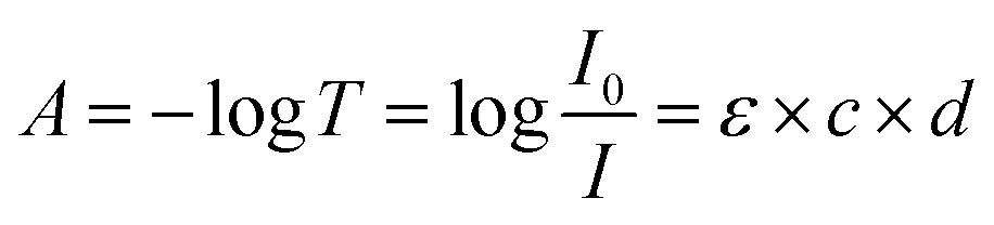
Fig. 1 shows the detailed hardware information of the applied UV-vis spectrophotometer platform in this article, which has been discussed in our previous study.³² The light from the light source, collimated by a group of lenses, irradiates into the double-optical-path structure. The light is received by the CMOS linear image sensor after passing through the focusing lens and gratings. The light into the upper path, called measurement light, passes through the sample pool, and absorption occurs. According to Lambert–Beer's law, absorption can be calculated by the following formula:where A represents the absorption, I₀/I is the intensity of the measuring light beam that is accepted by the CMOS sensor before/after passing through the sample; ε is the molar absorption coefficient; c is the concentration of the measured solution, and d is the path length of the measuring beam in the sample. Therefore, if the optical length is constant, a certain proportional relation exists between the absorption peak and the concentration of the measured solution. In this paper, we focused on the nitrate solution and the COD solution.³³

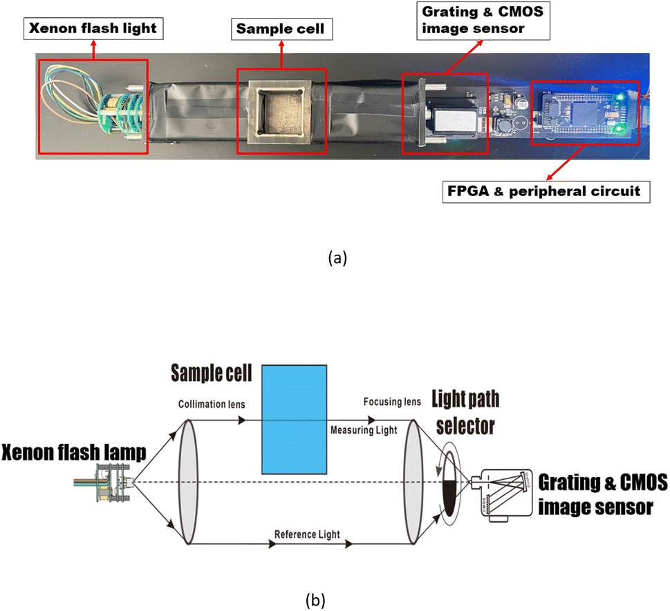Fig. 1 The implemented spectrophotometer platform incorporates a linear CMOS image sensor chip and FPGA microcontroller (a) and a schematic view of the fused double-beam structure (b).

2.2 Dataset

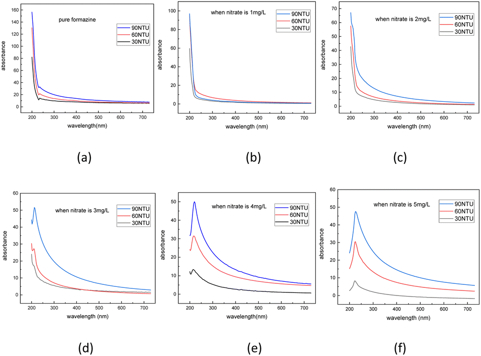
The dataset used in this study is comprised of UV-vis absorption spectra (200–750 nm) of 0–5 mg L⁻¹ nitrate solution and 0–70 mg L⁻¹ equivalent COD solution mixed with 0–90 NTU Formazin turbidity solution. The nitrate solution of different concentrations was prepared by dissolving potassium nitrate into the deionized water, which was supplied by a MilliQ water purification system (Millipore Corporation, Billerica, MA, USA). Meanwhile, the COD solution of different concentrations was prepared by dissolving the potassium hydrogen phthalate into the deionized water. All nitrate/COD concentrations mentioned below are expressed by converting the potassium nitrate solution/potassium hydrogen phthalate solution concentrations to equivalent nitrate/COD concentrations. The UV-vis absorption spectra in Fig. 2 were acquired spectrophotometer platform described in Section 2.1. A total of 480 700 UV-vis absorption spectra dataset was sourced by adding the single substance (nitrate/COD) solution spectra to different turbidity disturbances. The spectra of the single substance solution were expanded by applying the cubic spline interpolation method to the concentration gradient groups. In the actual water environment, due to the complexity of the substances in the water, the absorptivity of the different substances in the absorption spectra has a presence of interactions. Thus, it is usually not accurate to calculate the total absorption spectra by simply adding the solo absorption of each substance. To ensure that the influence, which the different turbidity brings to the nitrate/COD absorption spectra, is identical to the natural scenario, a new concept called Turbidity Residual Spectra (TRS), is proposed in this paper. As a result, 200 000 nitrate spectra and 280 700 COD spectra under the turbidity disturbance were generated and further split into a training set and a test set.

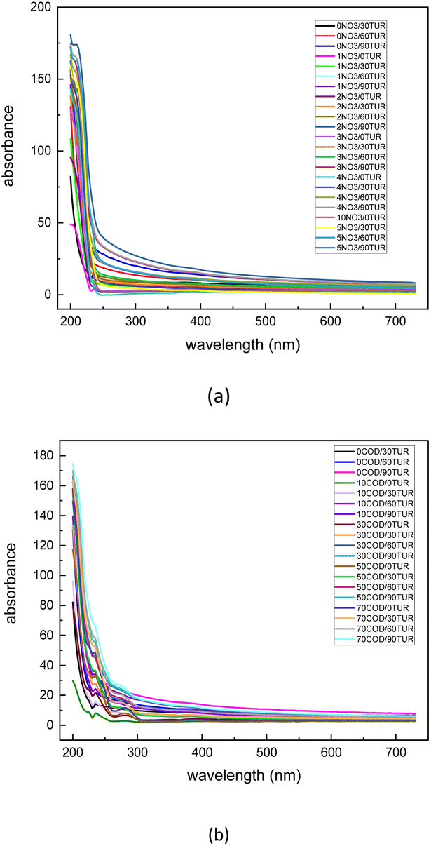Fig. 2 Measured original nitrate (a) and COD (b) absorption spectra with turbidity disturbance.

2.3 Partial least squares regression

PLSR analysis was performed in this study as the baseline method to compare the effect of the DL model performance. The PLSR was implemented using the partial least squares regression (PLSR) algorithm, which is a supervised method suitable for the large and unbalanced dataset with no obvious differences between the samples. The PLSR algorithm starts with calculating two unnormalized weights u and v, so that they maximize the covariance between the projected X matrix and the projected target Y. The scores are obtained by projecting X matrix and Y matrix on the singular vectors i.e. ξ = X·u and ω = Y·v then the loadings vectors are obtained by regressing X and Y on ξ. After deflating X and Y to subtract the variation extracted by the current number of components, we have scores matrices corresponding to the projection of the training data X and Y, respectively. After transforming X into X̄ and Y into Ȳ, using the rotation matrix P_X, P_Y which satisfied X̄ = XP_X, Ȳ = YP_Y, the targets of some data X can be predicted by looking for a coefficient matrix β such that Y = Xβ. PLSR algorithms find the fundamental relations between two matrices (X and Y) and project both X and Y into a lower-dimensional subspace such that the covariance between transformed (X) and transformed (Y) is maximal. In this work, 10-fold cross-validation was used to determine the optimal number of components for the final PLSR model, and the number of components was set to 20 based on the cross-validation result. The PLSR analysis was carried out using the “PLSRegression” function in python's cross decomposition module of the scikit-learn library.

2.4 Deep learning modeling

Dataset features suitable for the CNN method should meet the local correlation principle, which is to say, the data feature is mainly reflected in the local and can be extended from the local to the whole. The spectral sequence is equivalent to a long image (2600 points). When judging the properties of the characteristic peak from the absorption spectra sequence, it is the small pixel area adjacent to the peak that plays a key role, while the distant pixels in the spectra have a weak correlation. Thus, the spectra dataset meets the local correlation principle and we can apply CNN to the spectra sequence. It is also possible to apply recurrent neural network (RNN) models such as LSTM to the spectra sequence. However, the RNN method is not able to run in a parallel structure. Therefore, the data processing speed of RNN is unbearable for such a long spectra sequence.

The application of modern convolutional neural networks (CNN) generally consumes billions of parameters, which leads to a tremendous space complexity of the network model. Thus, it is crucial to utilize parallel computing technology to realize the acceleration and lightweight of the CNN model deployment. A method based on hardware improvement has been applied in this research. Moreover, the convolution procedure itself can be accelerated by choosing a proper convolution algorithm.

When a convolution kernel with dimension length d can be expressed as the exterior product of d vectors (each dimension contains one vector), this kernel is called the separable kernel. Applying the naïve convolution method to the separable kernel is quite inefficient for the final convolution result is equivalent to the combination of d one dimension convolution (each convolution using one of the d vectors). The combination method is faster than using the exterior product of a convolution kernel with dimension length d. Meanwhile, it takes fewer parameters to express the kernel into the vectors. For example, if the kernel's width is w elements in every dimension, the space and time complexity of the naïve convolution method is O(w^d), while the space and time complexity of the separable convolution method is O(w × d).

A 1-dimensional convolutional neural network (1D-CNN) deep learning (DL) architecture inspired by ref. 34 was used for model training and testing. A summary of the architecture is presented in Fig. 3, where 6 feature extraction layers were created with one spectrum input layer and one final regression result output layer. The spectra data is recognized by identifying absorption peaks' position and intensity, which, in general, are features with a large difference. To identify such features, maximum pooling was used for all pooling, and the Relu function (Relu(x) = max(x,0)) was used for the activation function. A max-pooling layer was added after each 1-D convolution block to reduce the dimension of each layer's output data as well. Each feature extraction layer contains a 1-D convolution block whose output dimension increases from 16 to 128, followed by the max pooling layer whose pool size and strides were both 2. With this combination in each layer, all features were retained, and then only the most “important” features in the local region are retained by pooling to achieve the purpose of down-sampling, and the obtained features are intuitively more accurate. Due to the relatively long spectral sequence (2600 dimensions), a double-channel-based structure was implemented to the 1D-CNN block to reduce the space and time complexity of the convolution calculation. Some tricks were also adopted to the model: for each convolution kernel in the 1-D convolution block, the kernel size was set as 3, dilated convolution was used, and the dilation rate was 1, 2, 4, respectively in each convolution kernel, and the number of 1-D convolution blocks was as large as possible. Another convolution kernel was used whose size was set as 1 to reconcile the input and the output of the block so that their shape remains consistent. For the nitrate dataset, 200 000 spectra samples were further split into 199 000 training and 1000 test sets using the “test_train_split” function from “SciKit-learn”. And for the COD dataset, 280 700 spectra samples were split into 279 700 training and 1000 test set.

Fig. 3 A summary of the double channel 1-D convolution neural network consisting of six convolutional layers with double parallel kernels for feature extraction, five max pooling layer, a single flatten layer, and a single fully connected layer with linear function for regression.

The model weights were optimized with an adaptive Adam optimizer. The mean squared error and coefficient of determination were used as the loss function and accuracy function to train the network. A batch size of 20 was used to get the best performance of the training procedure³⁵ and each model was trained up to 50 epochs with 500 steps per epoch. After every 50 epochs were finished, the learning rate was lowered by using different Adam optimizers. To have a fair comparison for different pre-processing techniques, the same architecture settings were used.

All analyses were carried out using Tensorflow GPU 2.6.0 using the dual Geforce RTX 3090 (Nvidia Corporation, Santa Clara, California, USA), under the environment of CUDA 11.2, using a small server computer equipped with a 2.20 GHz Intel® Xeon® Silver 4210 CPU (Intel Corporation, Santa Clara, CA) and 32 GB RAM, running Ubuntu 9.4.0 operating system and python 3.8.2.

3. Results

3.1 Spectral profiles and dataset augmentation

A convolutional neural network, that is capable of classifying objects robustly even if it is placed in a different place, is identified to have the property of invariance. In this paper's scenario, to be more specific, the property of invariance is reflected in the model's ability to accurately invert solute concentrations despite disturbances from different turbidity levels. By performing dataset augmentation, we can stop the neural network from learning irrelevant features (e.g. spectral features due to turbidity) and radically improve the overall performance.³⁰ In this research, considering the features of the spectra data, a new interpolation method was used to realize dataset augmentation.

Due to the non-linearity of Lambert's law, the effect of turbidity on the absorption spectra cannot be simply understood as the result of superimposing the turbidity spectrum on the solute spectrum.³⁶ In other words, the effect of turbidity on the absorption spectra can vary at different solute concentrations. To better understand the influence of turbidity brings to the absorption spectra under different solution concentrations, the absorption spectra of the substances before and after the effect of turbidity at each concentration were measured, and the difference between the two spectra was made to assess the contribution of turbidity to the spectra at different solution concentrations. The difference between the two spectra is called Turbidity Residual Spectra (TRS). Following the same procedure, the discrete TRS at each concentration was calculated, and the results are shown in Fig. 4.

Fig. 4 Discrete dataset of turbidity residual spectra under COD concentration of 10 mg L⁻¹ (a), 30 mg L⁻¹ (b), 50 mg L⁻¹ (c), and 70 mg L⁻¹ (d).

The turbidity residual spectra dataset was then expanded by applying the cubic spline interpolation method in the function “interpolate.interp1d()” in the python library “SciPy”. As depicted in Fig. 5, to obtain a continuous TRS dataset, the interpolation operation was used twice respectively for turbidity concentration filling and COD concentration filling, so that the corresponding TRS data ranges from 0–90 NTU can be found regardless of the COD concentration (0–70 mg L⁻¹). The interpolation operation was first applied in the turbidity values at each separate COD concentration and then applied in the COD concentration at each turbidity value interpolated before. The final continuous dataset structure is depicted in Table 2.

Fig. 5 Interpolation operation used twice respectively for turbidity concentration filling (a) and nitrate concentration filling (b).

Table 2 Continuous dataset structure of turbidity residual spectra in COD solution

Residual turbidity spectrum
COD concentration (mg L^−1)	Turbidity (NTU) residual turbidity spectrum
	0	0.225	⋯	30	⋯	60	⋯	90
0		⋯	⋯		⋯		⋯
0.1	⋯	⋯	⋯	⋯	⋯	⋯	⋯	⋯
⋯	⋯	⋯	⋯	⋯	⋯	⋯	⋯	⋯
10	⋯	⋯	⋯		⋯		⋯
⋯	⋯	⋯	⋯	⋯	⋯	⋯	⋯	⋯
30	⋯	⋯	⋯		⋯		⋯
⋯	⋯	⋯	⋯	⋯	⋯	⋯	⋯	⋯
50	⋯	⋯	⋯		⋯		⋯
⋯	⋯	⋯	⋯	⋯	⋯	⋯	⋯	⋯
70		⋯	⋯		⋯		⋯

---

As depicted in Fig. 6, the discrete TRS dataset under different nitrate solutions was calculated by following the same steps. Then the dataset was expanded using the same interpolation method, the interpolation result is shown in Table 3.

Table 3 Continuous dataset structure of turbidity residual spectra in nitrate solution

Residual turbidity spectrum
Nitrate concentration (mg L^−1)	Turbidity (NTU) residual turbidity spectrum
	0	0.225	⋯	30	⋯	60	⋯	90
0		⋯	⋯		⋯		⋯
0.1	⋯	⋯	⋯	⋯	⋯	⋯	⋯	⋯
⋯	⋯	⋯	⋯	⋯	⋯	⋯	⋯	⋯
1	⋯	⋯	⋯		⋯		⋯
⋯	⋯	⋯	⋯	⋯	⋯	⋯	⋯	⋯
2	⋯	⋯	⋯		⋯		⋯
⋯	⋯	⋯	⋯	⋯	⋯	⋯	⋯	⋯
3	⋯	⋯	⋯		⋯		⋯
⋯	⋯	⋯	⋯	⋯	⋯	⋯	⋯	⋯
4	⋯	⋯	⋯		⋯		⋯
⋯	⋯	⋯	⋯	⋯	⋯	⋯	⋯	⋯
5		⋯	⋯		⋯		⋯

---

Fig. 6 Dataset of turbidity residual spectra under nitrate concentration of 0 mg L⁻¹ (a), 1 mg L⁻¹ (b), 2 mg L⁻¹ (c), 3 mg L⁻¹ (d), 4 mg L⁻¹ (e), 5 mg L⁻¹ (f).

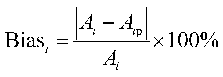
To further validate the accuracy of the dataset augmentation method, the absorption spectra of a 5 mg L⁻¹ nitrate and a 50 mg L⁻¹ COD solution were then tested at turbidity of 45 NTU, and the test results were compared with the simulation spectra using the indicators of standard bias. The standard bias at each wavelength is calculated using the following formula:

in which, A_i is the tested absorbance at the wavelength i, A_ip is the simulated absorbance at the wavelength i. One of the interpolation spectral data of nitrate and COD solutions are depicted in Fig. 7(a) and (c). The calculation results of normalized bias between the interpolation spectra and true spectra of nitrate and COD are depicted in Fig. 7(b) and (d). For both scenarios in nitrate and COD solutions, the simulated spectra result showed a high level of accuracy. More specifically, in the worst case of the COD solution spectra at the wavelength of 300 nm, the bias was still below 6%, and the average bias levels in the COD solution were at 4.1%. As for the nitrate spectra case, due to the simplicity of the nitrate spectra (the spectra data shows a smoother curve), the simulated spectra results gained a better accuracy, and the average bias level reached 1.6%.

Fig. 7 Interpolation spectra and true spectra of nitrate (a) and COD (c) and normalized bias between the interpolation spectra and true spectra of nitrate (b) and COD (d).

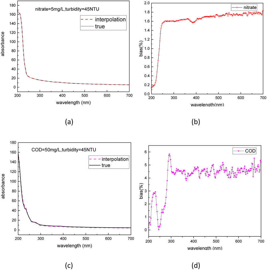
A distribution summary of reference nitrate and COD solution values in test and training sets is presented in Fig. 8. The dataset was produced by adding the corresponding turbidity residual spectra to the nitrate/COD absorption spectra at different concentrations. The nitrate and COD concentration of the test set was well represented in the method of random sampling using the ‘sample’ function in the python library of “pandas”.

Fig. 8 Distribution of nitrate (a) and COD (b) solution for the test and training sets.

3.2 Convolution neural network vs. partial least-squares

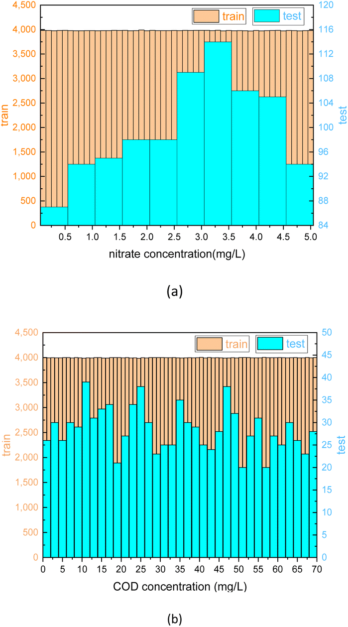
Fig. 9 shows the evolution of the loss and accuracy rate of the model during the training process of 1D-CNN. The coefficient of determination was used as an indicator of model accuracy and the mean square error (MSE) was used as an indicator of model loss. A closer look at the trends in loss and accuracy reveals a small leap when the training epoch arrives at 50, due to an adjustment in the learning rate (from 10⁻² to 10⁻³). At the epoch of 100, even though the learning rate of the model was adjusted to a smaller value (from 10⁻³ to 10⁻⁴), the loss and learning rate remained essentially unchanged, which indicates the model is about to converge. It finally takes 1391 seconds for the 1D-CNN model to complete the whole 150-epoch training (about 9 seconds per epoch). The MSE and the coefficient of determination of the model nearly respectively reached 0 and 1 at the end of the training process. Therefore, it can be concluded that at this point, the model training converges to convergence for the current training sets. The model was trained separately for COD nitrate datasets. Thus, two models were produced for the corresponding datasets.

Fig. 9 Trends in loss (MSE) and accuracy (coefficient of determination) of the model during the training procedure.

The best-performing models were saved after the training process was completed. To further evaluate the performance of the model, 1000 test sets of COD and nitrate spectra data produced in 3.1 were sent into the two corresponding models. In Fig. 10 and 11, the comparison was made between the PLSR and 1-D CNN method for predicted regression results of COD and nitrate solution concentration using the test sets. The true values and the predicted regression values using the two different methods are directly shown in Fig. 10(a), (c), 11(a) and (c). If the round point and the triangle point in the figure overlap, it can be concluded that the regression is highly accurate. Thus, as can be seen from the figure, in both COD and nitrate solutions, the bias between the true values and the predicted regression values in the CNN model was much smaller than it was in the PLSR model. To further quantify the model regression accuracy, a scatter plot was drawn using the true values as the horizontal axis and the predicted regression values as the vertical axis, and the linear analysis between the true values and predicted regression values were made as shown in Fig. 10(b), (d), 11(b) and (d). It can be seen from the scatter plot that the higher the regression accuracy is, the closer to one the slope of the fitting line is. Thus, the accuracy of the model can be evaluated by checking the linearity and the slope in the linear analysis result. The R-square in the CNN model for the linear analysis of nitrate and COD solution was 0.99943 and 0.99946, while in the PLSR model was 0.98869 and 0.99407. The slope in the CNN model for the linear analysis of nitrate and COD solution was respectively 0.99575 and 1.00021, while in the PLSR model was 0.98804 and 0.9935. Consequently, both indicators of slope and R-square reveal that the CNN model performs higher accuracy in nitrate solution and COD solution under random turbidity disturbance.

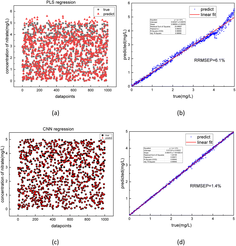Fig. 10 Comparison between predicted regression values and true values of nitrate solution using PLSR (a) and 1-D CNN (c) model with model accuracy evaluation on PLSR (b) and 1-D CNN (d) using the linear regression method.

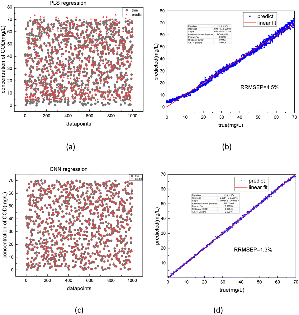Fig. 11 Comparison between predicted regression values and true values of COD solution using PLSR (a) and 1-D CNN (c) model with model accuracy evaluation on PLSR (b) and 1-D CNN (d) using the linear regression method.

Moreover, RRMSEP was also used as an evaluation indicator for the regression model,^37,38 the RRMSEP can be calculated using the following formula:

in which, y_i is the true concentration value of the sample i, y_ip is the predicted regression concentration value of the sample i in the test sets. Parameter m is the total sample quantities in the test sets. Thus, the lower the RRMSEP is, the closer the true value of the predicted regression value is. The calculation results indicate that the RRMSEP of the CNN model for nitrate and COD solution was respectively 4.7% and 3.2% lower compared to the PLSR model.

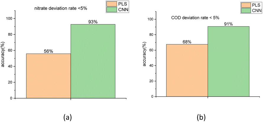
To compare the accuracy of the two models more intuitively, it is defined that the group, whose bias between the true values and the predicted regression values is less than 5%, is the group with the correct judgment. The comparison result for the nitrate and COD solution is depicted in Fig. 12. The figure shows that the accuracy of nitrate concentration regression was increased from 56% of the PLSR model to 93% of the CNN model and the accuracy of COD concentration regression was increased from 68% of PLSR model to 91% of CNN model.

Fig. 12 Accuracy comparison between PLSR and 1-D CNN method for the result of nitrate (a) and COD (b) solution concentration regression using the test sets.

When applying the PLSR algorithm, the non-linearity appeared between the predicted regression and true values of both COD and nitrate solutions at high-concentration groups. This is due to the deviation from linearity in the absorption spectrum peak at high solute concentrations, which is caused by the CMOS image sensor showing different photoelectric conversion efficiencies at different light intensities and different wavelengths.³⁹ On the other hand, the CNN method learned the non-linear deviation in the absorption spectrum peak generated by the hardware system of the spectrometer from a large dataset and successfully corrected this deviation.

To better showcase the performance of our CNN method, the regression results of other non-linear methods such as SVR and k-nearest neighbor (KNN) method were added to the Table 4. Radial basis function (RBF) is used as the kernel function of the SVR method to handle the non-linear problems. The results indicated that the SVR is the most time-consuming method while processing the long spectral data in the large size scale of the dataset, while KNN is the most time-saving method at the cost of a low accuracy rate.

Table 4 Different modelling regression results of nitrate/COD dataset

Algorithm	Average RRMSEP	Average result accuracy rate	Processing time (training time included)
Partial least squares regression (PLSR)	5.3%	61.5%	657 seconds
Support vector machine regression (SVR)	4.6%	86.4%	1569 seconds
k-Nearest neighbor (KNN)	5.5%	59.4%	235 seconds
Double-channel 1-D convolution neural network (1-D CNN)	1.3%	92%	1395 seconds

---

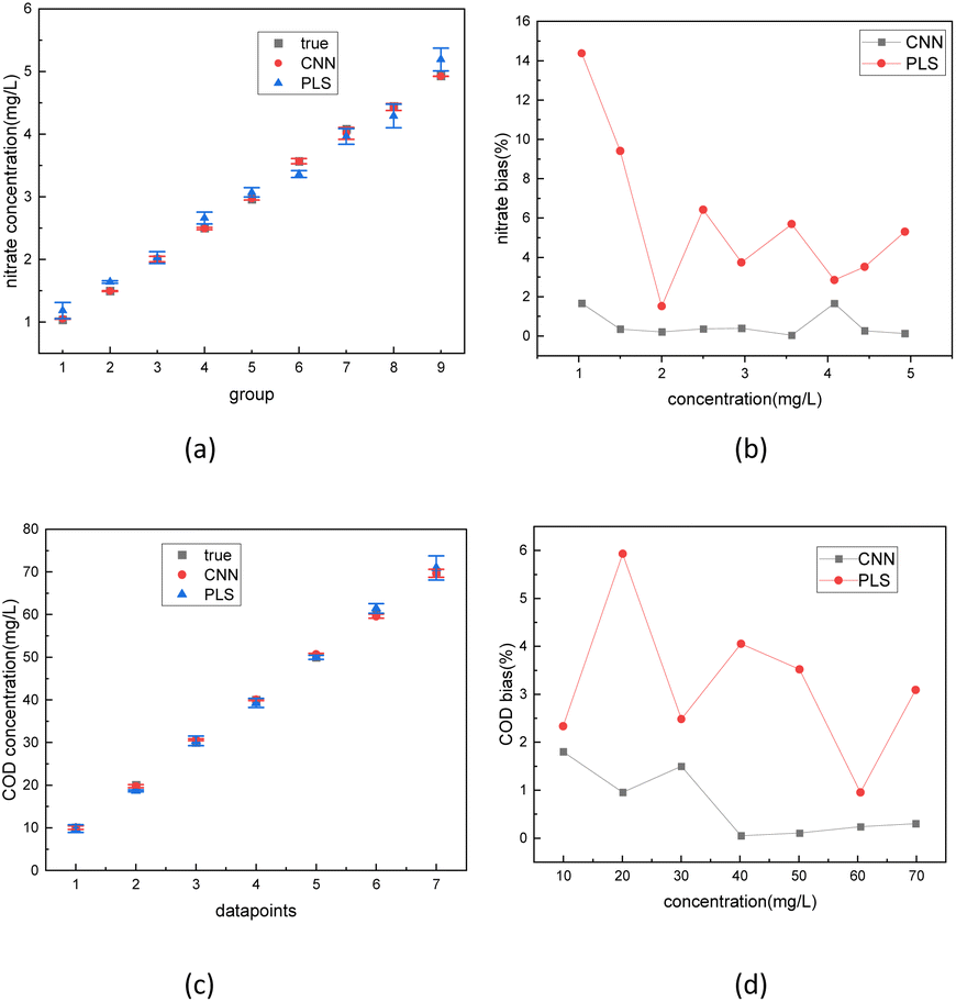
Finally, the absorption spectra of nitrate solutions and COD solutions blended with 10, 50, and 80 NTU turbidity solutions were tested. The spectrum data was sent separately into the trained 1D-CNN model and PLSR model. The regression results of two different models are depicted in Fig. 13. The error bar in Fig. 13(a) and (b) represents the error level of three regression results (under 10, 50, 80 NTU) in each concentration. The bias in Fig. 13(c) and (d) calculated by the formula (2) represents the relative deviation between the true values and the predicted regression values of the solute. The results indicate that the CNN had an error rate of less than 2% for both nitrate and COD concentration in actual solution tests. In comparison, using the PLSR method, the worst bias rate in actual solution tests was 15%.

Fig. 13 Regression results of the actual nitrate (a) and COD (c) solutions blended with 10, 50, and 80 NTU turbidity solutions with regression accuracy comparison between PLSR and 1-D CNN method on nitrate (b) and COD (d) solution.

From the demonstration of the modeling process and the analysis of the regression results, it can be concluded that the advantage of the proposed CNN method is that by combining the dataset augmentation method and CNN method, the turbidity interference is successfully excluded during spectrometric quantification of nitrate/COD solution without any spectral pre-treatment. However, the proposed method still has its drawback, that its application scenarios are highly dependent on the training dataset.

4. Conclusions

This study introduced an analysis method for the absorption spectra of nitrate and COD solution under a random turbidity disturbance scenario. The method is based on the structure of 1-D CNN, and some improvement to the network structure has been made such as double-channel transmission, dilated convolution, and diminishing Adam optimizer to adapt the model to the relatively long spectral sequence (2600 points). To obtain a more realistic spectral dataset for the CNN model under random turbidity disturbance, the concept of turbidity residual spectrum was introduced. On this basis, the cubic spline interpolation operation was applied twice respectively for the TRS dataset and pure solution dataset so that a continuous spectrum dataset of different solute concentrations under different turbidity disturbances can be acquired. The evaluation result of the spectrum bias between the simulation and the tested nitrate solution was below 2% in all wavelengths, while it was 4.1% on average in all wavelengths in the COD solution. The result indicates that this dataset augmentation method successfully restored the spectrum data of the nitrate and COD solution under different turbidity disturbances.

The augmented training dataset was then fed into the PLSR model and the CNN model. The training results of the two models were compared. The results show that the R-square value for the PLSR model between the true values and predicted regression values of nitrate and COD solution were 0.98869 and 0.99407, while they were 0.99943 and 0.99946 for the CNN model. Compared to the PLSR model, the value of RRMSEP for the CNN model was reduced from 6.1% to 1.4% in nitrate solution and from 4.5% to 1.3% in COD solution, and the accuracy of the regression result for the CNN model was increased from 56% to 93% in nitrate solution and 68% to 91% in COD solution. At last, the absorption spectra of prepared nitrate and COD solutions in more groups blended with different turbidity solutions were tested. The test result shows that the 1D-CNN model performed an error rate of less than 2% in both nitrate and COD solutions, while the worst bias rate in the PLSR method was 15%. All the test results indicate that the 1D-CNN model can successfully extract and quantify the characteristic information of nitrate/COD solution from the absorption spectra under random turbidity disturbance and the 1D-CNN model showed higher regression accuracy compared to the PLSR method.

Author contributions

Investigation, methodology, formal analysis, writing – original draft, validation, Meng Xia; methodology, review & editing, funding acquisition, Gaofang Yin; supervision, conceptualization, funding acquisition, Nanjing Zhao; writing – review & editing, funding acquisition Ruifang Yang; investigation, Xiaowei Chen; investigation, Jingsong Chen.

Conflicts of interest

The authors declare no conflict of interest.

Acknowledgements

This research was funded by: National Natural Science Foundation of China grant number (61875254); Science and Technology Major Project of the Ministry of Science and Technology of Anhui Province, grant number (202003a07020007); Key Fusion Program of Special Foundation of President of Chinese Academy of Sciences Hefei Institutes of Physical Science, grant number (YZJJZX202009); Instrument and Equipment Function Development Program of the Chinese Academy of Sciences, grant number (E03HBF11291); National Key Scientific Instrument and Equipment Development Project, grant number (2017YFF0108402).

Notes and references

1. A. S. Elshall, et al., Groundwater sustainability: a review of the interactions between science and policy, Environ. Res. Lett., 2020, 15(9), 093004.
2. M. G. Uddin, et al., A comprehensive method for improvement of water quality index (WQI) models for coastal water quality assessment, Water Res., 2022, 219, 118532.
3. D. S. Thambavani and T. Mageswari, Water quality indices as indicators for potable water, Desalin. Water Treat., 2014, 52(25–27), 4772–4782.
4. Y. C. Guo, et al., Advances on Water Quality Detection by UV-Vis Spectroscopy, Appl. Sci., 2020, 10(19), 6874.
5. D. B. Hou, et al., Water Quality Analysis by UV-Vis Spectroscopy: A Review of Methodology and Application, Spectrosc. Spectral Anal., 2013, 33(7), 1839–1844.
6. Z. N. Shi, et al., Applications of Online UV-Vis Spectrophotometer for Drinking Water Quality Monitoring and Process Control: A Review, Sensors, 2022, 22(8), 2987.
7. X. S. Wu, et al., Study on an Online Detection Method for Ground Water Quality and Instrument Design, Sensors, 2019, 19(9), 2153.
8. G. Langergraber, N. Fleischmann and F. Hofstadter, A multivariate calibration procedure for UV/VIS spectrometric quantification of organic matter and nitrate in wastewater, Water Sci. Technol., 2003, 47(2), 63–71.
9. T. Tiecher, et al., Improving the quantification of sediment source contributions using different mathematical models and spectral preprocessing techniques for individual or combined spectra of ultraviolet-visible, near- and middle-infrared spectroscopy, Geoderma, 2021, 384, 114815.
10. H. Xue, et al., Highly selective colorimetric and electrochemical Pb2+ detection based on TTF-pi-pyridine derivatives, J. Org. Chem., 2005, 70(24), 9727–9734.
11. L. Guan, et al., Research on ultraviolet-visible absorption spectrum preprocessing for water quality contamination detection, Optik, 2018, 164, 277–288.
12. Y. T. Hu, Y. Z. Wen and X. P. Wang, Novel method of turbidity compensation for chemical oxygen demand measurements by using UV-vis spectrometry, Sens. Actuators, B, 2016, 227, 393–398.
13. M. L. Darder, et al., Comparing multifractal characteristics of soil particle size distributions calculated by Mie and Fraunhofer models from laser diffraction measurements, Appl. Math. Model., 2021, 94, 36–48.
14. J. J. Nichols and P. E. King-Smith, Thickness of the Pre- and Post–Contact Lens Tear Film Measured in vivo by Interferometry, Invest. Ophthalmol. Visual Sci., 2003, 44(1), 68–77.
15. K. J. S. Silva, et al., Visibility Graph Analysis of Particle Size Distribution During Flocculation for Water Treatment, Water, Air, Soil Pollut., 2021, 232(3), 86.
16. L. Ursica, et al., Particle size analysis of some water/oil/water multiple emulsions, J. Pharm. Biomed. Anal., 2005, 37(5), 931–936.
17. J. W. Li, et al., A turbidity compensation method for COD measurements by UV-vis spectroscopy, Optik, 2019, 186, 129–136.
18. G. Langergraber, et al., Monitoring of a paper mill wastewater treatment plant using UV/VIS spectroscopy, Water Sci. Technol., 2004, 49(1), 9–14.
19. D. Carreres-Prieto, et al., Evaluation of genetic models for COD and TSS estimation in wastewater through its spectrophotometric response, Water Sci. Technol., 2022, 85(9), 2565–2580.
20. L. Rieger, et al., Spectral in situ analysis of NO2, NO3, COD, DOC and TSS in the effluent of a WWTP, Water Sci. Technol., 2004, 50(11), 143–152.
21. J. W. Feng, et al., New Approach for Concentration Prediction of Aqueous Phenolic Contaminants by Using Wavelet Analysis and Support Vector Machine, Environ. Eng. Sci., 2020, 37(5), 382–392.
22. Y. Lu, et al., Detection of chlorpyrifos and carbendazim residues in the cabbage using visible/near-infrared spectroscopy combined with chemometrics, Spectrochim. Acta, Part A, 2021, 257, 119759.
23. C. Wolf, et al., Predicting organic acid concentration from UV/vis spectrometry measurements – a comparison of machine learning techniques, Trans. Inst. Meas. Control, 2013, 35(1), 5–15.
24. O. Rahmati, et al., Predicting uncertainty of machine learning models for modelling nitrate pollution of groundwater using quantile regression and UNEEC methods, Sci. Total Environ., 2019, 688, 855–866.
25. A. Torres and L. López-Kleine, UV-vis in situ spectrometry data mining through linear and non linear analysis methods, Dyna, 2014, 81(185), 190–196.
26. G. E. Hinton, S. Osindero and Y. W. Teh, A fast learning algorithm for deep belief nets, Neural Comput., 2006, 18(7), 1527–1554.
27. W. Ng, et al., Convolutional neural network for simultaneous prediction of several soil properties using visible/near-infrared, mid-infrared, and their combined spectra, Geoderma, 2019, 352, 251–267.
28. C. H. Cui and T. Fearn, Modern practical convolutional neural networks for multivariate regression: Applications to NIR calibration, Chemom. Intell. Lab. Syst., 2018, 182, 9–20.
29. X. J. Wu, et al., Quantitative analysis of blended corn-olive oil based on Raman spectroscopy and one-dimensional convolutional neural network, Food Chem., 2022, 385, 132655.
30. C. Shorten and T. M. Khoshgoftaar, A survey on Image Data Augmentation for Deep Learning, J. Big Data, 2019, 6(1), 60.
31. Y. Tang and C. Eliasmith, Deep networks for robust visual recognition, in ICML 2010 – Proceedings, 27th International Conference on Machine Learning, 2010, pp. 1055–1062.
32. M. Xia, et al., A Design of Real-Time Data Acquisition and Processing System for Nanosecond Ultraviolet-Visible Absorption Spectrum Detection, Chemosensors, 2022, 10(7), 282.
33. S. Asadollah, et al., River water quality index prediction and uncertainty analysis: a comparative study of machine learning models, J. Environ. Chem. Eng., 2021, 9(1), 104599.
34. G. Larsson, M. Maire and G. Shakhnarovich, FractalNet: ultra-deep neural networks without residuals, in 5th International Conference on Learning Representations, ICLR 2017 – Conference Track Proceedings, 2017.
35. N. S. Keskar, et al., On large-batch training for deep learning: Generalization gap and sharp minima, in 5th International Conference on Learning Representations, ICLR 2017 - Conference Track Proceedings, 2017.
36. W. Mantele and E. Deniz, UV-VIS absorption spectroscopy: Lambert-Beer reloaded, Spectrochim. Acta, Part A, 2017, 173, 965–968.
37. E. Gruner, M. Wachendorf and T. Astor, The potential of UAV-borne spectral and textural information for predicting aboveground biomass and N fixation in legume-grass mixtures, PLoS One, 2020, 15(6), e0234703.
38. D. Perez-Guaita, et al., Evaluation of infrared spectroscopy as a screening tool for serum analysis Impact of the nature of samples included in the calibration set, Microchem. J., 2013, 106, 202–211.
39. W. J. Deng, C. Y. You and Y. Z. Zhang, Spectral Discrimination Sensors Based on Nanomaterials and Nanostructures: A Review, IEEE Sens. J., 2021, 21(4), 4044–4060.

---