
 Open Access Article
 This Open Access Article is licensed under a Creative Commons Attribution-Non Commercial 3.0 Unported Licence
Modeling of Sandia Flame D with the non-adiabatic chemistry tabulation approach: the effects of different laminar flames on NOX prediction†
Chuanfeng Yue ab,
Jingbo Wang*ab and
Xiangyuan Liab
ab,
Jingbo Wang*ab and
Xiangyuan Liab
aCollege of Chemical Engineering, Sichuan University, Chengdu, 610065, P. R. China. E-mail: wangjingbo@scu.edu.cn
bEngineering Research Center of Combustion and Cooling for Aerospace Power, Ministry of Education, Sichuan University, Chengdu, 610065, P. R. China
First published on 6th February 2023
Abstract
The effects of different one-dimensional laminar flames on the prediction of nitrogen oxide (NOX) emission in Sandia Flame D are numerically investigated using a flamelet method in the present work. In addition to the basic control variables of the mixture fraction and the reaction progress variable for chemistry tabulation in this combustion model, two additional variables of mixture fraction variance and enthalpy loss are added to the control variable space to improve prediction accuracy of the NOX pollutant. The former variable of mixture fraction variance is used for the presumed probability density function integration, and the latter takes into account the non-adiabatic effect. Two flamelet libraries are generated based on the one-dimensional unstretched premixed flame and the one-dimensional counterflow diffusion flame, respectively. An additional transport equation for the mass fraction of nitrogen oxide (NO) is solved for improving prediction accuracy. The unsteady Reynolds-averaged Navier–Stokes (URANS) simulation results are compared and analyzed with experimental data. The simulation results show dependence on the type of laminar flame. In the four-dimensional control variable space, the results with steady unstretched premixed flame indicate great agreement on the predictions of temperature and NO field. The computational method proposed in the present work sheds light on the high-precision combustion numerical simulation of NOX emission.
1. Introduction
With the increasing attention of pollution issues, the emission reduction of pollutants such as nitrogen oxides (NOX) has become one of the important indicators in the development of gas turbines and internal combustion engines. While computational fluid dynamics (CFD) is utilized as a powerful design approach in the motivation to design high performance and clean burners,1 one-step or global reaction mechanisms are widely used in engineering simulation applications due to limited computational resources. However, NOX emission predictions given in these conditions are inaccurate due to the oversimplified chemical mechanism leading to incomplete related reactions.2–8 High-precision chemical mechanisms frequently containing thousands of species for hydrocarbons3 bring unacceptable computational cost. Therefore, the application of the high-precision chemical kinetic models in combustion simulations has become an important research topic.4–13Recent advances in combustion modeling to reduce the computational cost of application of detailed chemical kinetics are the development of flamelet-like models,14–16 such as flame prolongation of intrinsic low-dimensional manifolds (FPI),17 steady laminar flamelet model (SLFM),18 flamelet/progress variable (FPV)19 and flamelet generated manifold (FGM).20 These combustion models share the same basic assumption that the high-dimensional real flame consists of a series of low-dimensional flamelets. It means that the species distribution in turbulent combustion (high-dimensional) can be estimated by the low-dimensional manifolds (LDM). The FGM model developed by Oijen et al.21 have two basic control variables of mixture fraction  and progress variable
  . The FGM library is built by mapping thermophysical parameters such as species mass fractions in different states to the control variable space. However, the errors are inevitable for the operation of directly look-up NOX mass fraction in the library due to the different characteristic time scales of
  and NOX.6,22,23
Many works on NOX modeling with flamelet-like approaches have been reported in literature. Ihme et al.24 performed LES/FPV simulations of turbulent non-premixed flames. They found that NO emission (the main component of NOX emission) prediction could be improved by adding additional NO transport equation and modeling the consumption component in the NO source term separately. Considering the larger time scale of NO, Godel et al.22 proposed a novel  definition by additional including NOX species that could captures better NO evolution. Similarly, Akargun et al.25 built the extended FGM table by optimizing the definition of PV for key parameters such as soot and NOX for non-premixed combustion. Various tests of different ways to modeling NOX formation with FGM method are performed by Tang et al.,26 which indicated that the prediction of NO can be improved effectively by considering radiation. Due to some key parameters of the steady diffusion flamelet will affect the accuracy of simulation results, such as temperature and NO concentration, Yao et al.27 proposed a procedure to optimize flamelet parameters by using the surrogate assisted evolutionary algorithm. The LES/FGM simulation of CH4/NH3/air swirl flames28 demonstrated that the NH3 concentration, residence time and temperature are important factors to effect the concentration distribution of NO. Recently, Zhang et al.29 investigated the effect of transport properties on near-wall temperature by using uniform and non-uniform Lewis number (Le) in LES/FGM simulation.
According to the literature, the flamelet library can be constructed with one-dimensional laminar premixed flame or with one-dimensional laminar counterflow diffusion flame. The former is used to study flame propagation problems, and the latter is applicable to diffusion flames, auto-ignition and extinction (scalar dissipation rate plays a very important role). Generally, the first step is to determine which one-dimensional laminar flame is more similar to the flame structure in the CFD simulation when using a flamelet-like model for chemistry tabulation. However, there is no clear answer to this question, especially for the prediction of NOX emission. In present work, the effects of two one-dimensional laminar flames, unstretched premixed (UP) flame and counterflow diffusion (CD) flame, on the prediction of NOX emission in Sandia Flame D are investigated by unsteady Reynolds-averaged Navier–Stokes (URANS) method with a customized solver developed on the platform of OpenFOAM.30,31 Since the flamelet library generated with the basic variables of  and
and  cannot predict NOX emission well, present study takes into account the turbulence-chemical-radiation-interaction (TCRI) by adding additional control variables of mixture fraction variance and enthalpy loss. The rest of present work consists of three parts. Section 2 briefly introduces the mathematical methods of turbulent combustion, case configuration and numerical setup. The effect of the two flamelet libraries on flame structure and NOX emission are discussed in Section 3. The main findings are summarized in Section 4.
2. Methodology
2.1. Governing equations
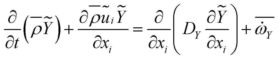
The solution strategy of using the URANS model and the chemistry tabulation approach to simulate the Sandia Flame D in current study is summarized as following steps:(i) With the definition of the variables of  ,
,  and enthalpy loss, a series of two kinds of laminar flames, UP flame and CD flame, are solved and transformed to obtain the corresponding laminar flamelets, respectively.
(ii) The variance of the mixture fraction is defined and add to the control variables space for the β probability density function (β-PDF) integration. And the turbulent flamelets library is obtained by presumed PDF integration.
(iii) Solving the governing equations including control variables in CFD solver and thermo-chemistry variables are updated by the flamelet library.
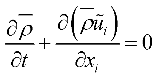
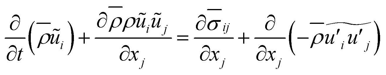
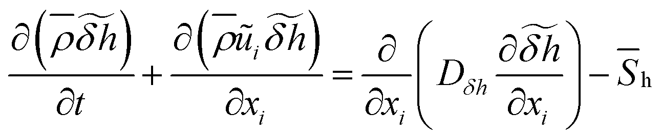
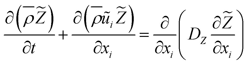
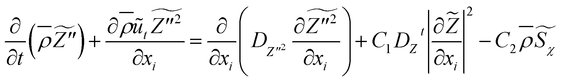
The governing equations for mass, momentum, control variables are expressed as follows:
 | (1) |
 | (2) |
 | (3) |
 | (4) |
 | (5) |
 | (6) |
 are density, velocity, enthalpy loss, mixture fraction, variance of mixture fraction and progress variable, respectively. The superscript –, ∼ means unweighted average and density weighted average. Tensor σij defined as
| σij = 2μ(Sij − Skkδij/3) − pδij | (7) |
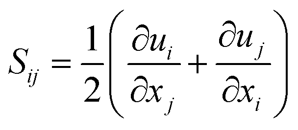 | (8) |
According to Boussinesq's hypothesis, Reynolds stress Rij is given by
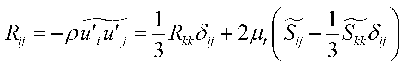 | (9) |
 and
and  are effective dynamic viscosity of mixture fraction, variance of mixture fraction, and process variables, respectively. According to the unity Lewis number assumption, they can be expressed as
 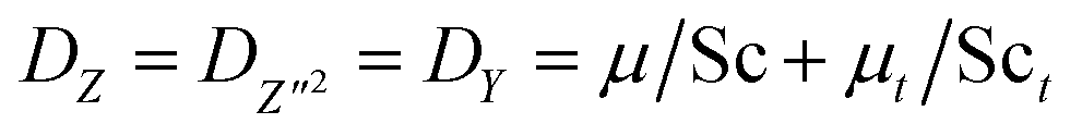 with r = 1.0, Sct = Prt = 0.7. μ and μt are molecular and turbulent viscosity, μ = λ/Cp, μt = ρCμk2/ε. k is the turbulent kinetic energy, ε is the turbulent dissipation rate for the standard k–ε turbulence model.32 Compared with the predictions of the k–ω-SST model that is commonly used in engineering simulation, the standard k–ε model gives more accurate temperature peaks and corresponding reasonable NO peaks on the central axis. The results are shown in Fig. S1 of the ESI.† So turbulent scalar dissipation rate of mixture fraction
  is defined as
  . For constant numbers in eqn (5), C1 = C2 = 2.0. The radiation effect is considered in present work and the radiation model of optical thin model (OTM) is adopted.33,34
 ![[S with combining macron]](https://www.rsc.org/images/entities/i_char_0053_0304.gif) h is source term of radiation.
h is source term of radiation.| Sh(T, species) = 4σ(T4 − Tb4)∑(piap,i) | (10) |
2.2. Flamelet library generation and TCRI
The two one-dimensional laminar flames are calculated using FlameMaster.35 A series of mixture fraction are used to change the equivalent ratio of inlet boundary for building UP library. Mixture fraction
  is defined by Bilger's formulation.36
 | (11) |
 space. Then flamelets are obtained by transforming all the one-dimensional flame solutions into the
  space, where
  is defined by the linear combination of steady state products of CO2 and CO.
 | (12) |
To incorporate non-adiabatic effects, a third parameter δh related to enthalpy loss is introduced. The enthalpy defect is defined by the difference between the enthalpy of the initial mixture for adiabatic and non-adiabatic conditions,
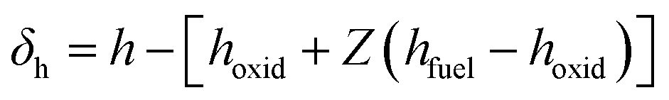 | (13) |
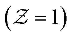 and the oxidation side
 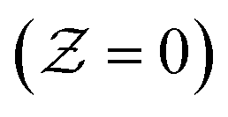 are,
are,
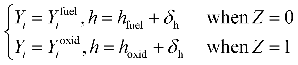 | (14) |
The same strategy applies to the enthalpy conditions of the UP flame, but different mixture fractions imply a range of equivalence ratios, where fuel and oxidant get mixed side,
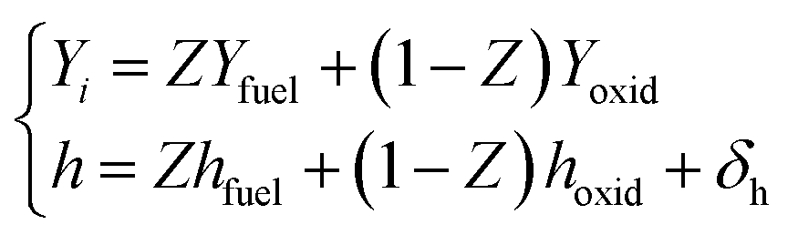 | (15) |
Finally, the TCRI is accounted through the joint PDF of the independent variables. By applying β-PDF to mixture fraction and δ-PDF to other control variables, the Favre-averaged/filtered scalars ϕ is expressed as
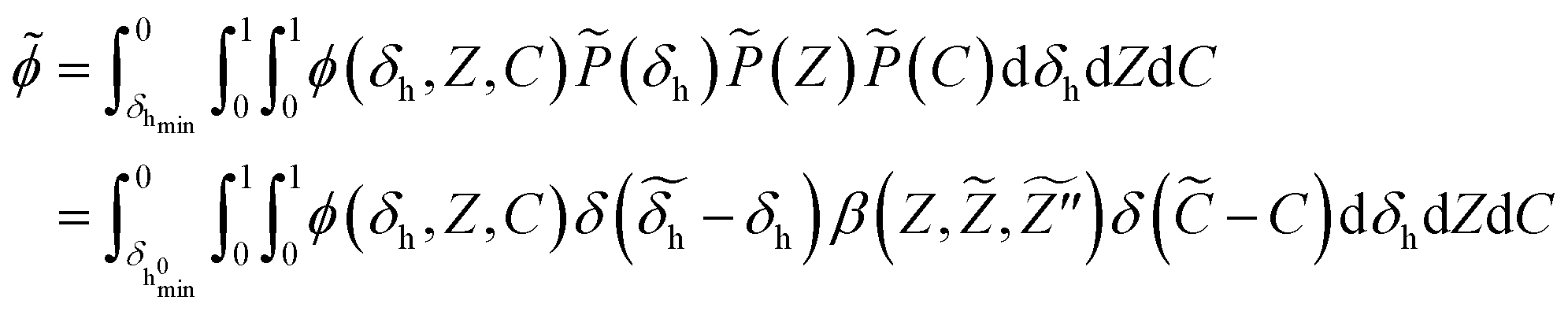 | (16) |
 denotes normalized progress variable.
Based on the above methods, the pressure-based compressible solver is developed on the platform of OpenFOAM.38 The pressure-velocity-density is solved through the PIMPLE algorithm.38 The spatial accuracy is formally second-order.
2.3. Solution of NOX
In the composition of NOX emission, the amount of NO is one order of magnitude higher than that of the other components.16 Therefore, the content of NO generally represents the NOX emission. After trying various methods, an additional transport equation of NO mass fraction, as suggested by Ihme et al.24 in their turbulent premixed flame simulation, gets solved in present work in order to improve the prediction accuracy.
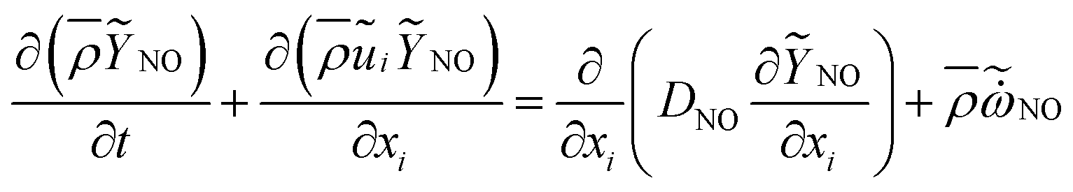 | (17) |
 , is obtained by interpolation in flamelet library. See Section 3.1 for details on establishment of the
  database. When the enthalpy loss is 0 kJ kg−1, the distribution of
  in the
  space is shown in Fig. 4. The detailed CH4/air mechanism adopted in present work is GRI-2.11 (ref. 39) that shows more accurate results on NOX emission40 compared to GRI-3.0.41
2.4. Computational domain and numerical setup
Present investigation case is Sandia Flame D42 and the burner schematic is shown in Fig. 1. The axisymmetric piloted burner has a main jet inner diameter (D) of 7.2 mm. The pilot annulus inner diameter and outer diameter is 7.7 mm and 18.2 mm, respectively. The burner outer wall diameter is 18.9 mm. Computational domain is a wedge with 5° and its axial and radial length is 80D × 20D. Grid cells around the axis and has a resolution of 162 × 1 × 500. The mesh has a minimum grid of 0.125 mm and a total cell number of 81![[thin space (1/6-em)]](https://www.rsc.org/images/entities/char_2009.gif) 000. Based on Reynolds numbers of 22400, air-coflow, piloted jet and main fuel jet have bulk inflow velocity of 0.9 m s−1, 11.4 m s−1 and 49.6 m s−1, and have inflow temperature of 291 K, 1880 K and 294 K, respectively. The velocities of coflow and main fuel jet are under the standard state of 294 K, 0.993 atm. The pilot bulk velocity is estimated from the specified conditions, the flow area of the pilot annulus and the measured mass flow rates. The ambient pressure is 0.996 atm. Fuel is CH4/air mixtures with a volume ratio of 1:3
000. Based on Reynolds numbers of 22400, air-coflow, piloted jet and main fuel jet have bulk inflow velocity of 0.9 m s−1, 11.4 m s−1 and 49.6 m s−1, and have inflow temperature of 291 K, 1880 K and 294 K, respectively. The velocities of coflow and main fuel jet are under the standard state of 294 K, 0.993 atm. The pilot bulk velocity is estimated from the specified conditions, the flow area of the pilot annulus and the measured mass flow rates. The ambient pressure is 0.996 atm. Fuel is CH4/air mixtures with a volume ratio of 1:3  . The piloted jet is burned mixtures containing C2H2, H2, air, CO2 and N2
  . The pressure inlet boundary condition adopts the Neumann condition, and the pressure outlet boundary condition adopts the Dirichlet condition. The inlet boundary condition of other solution variables adopts Dirichlet condition, the outlet boundary condition adopts Neumann condition, and the wall adopts no-slip wall condition. Specifically, the k and ε use the wall function. Periodic boundary conditions are used on the left and right sides.
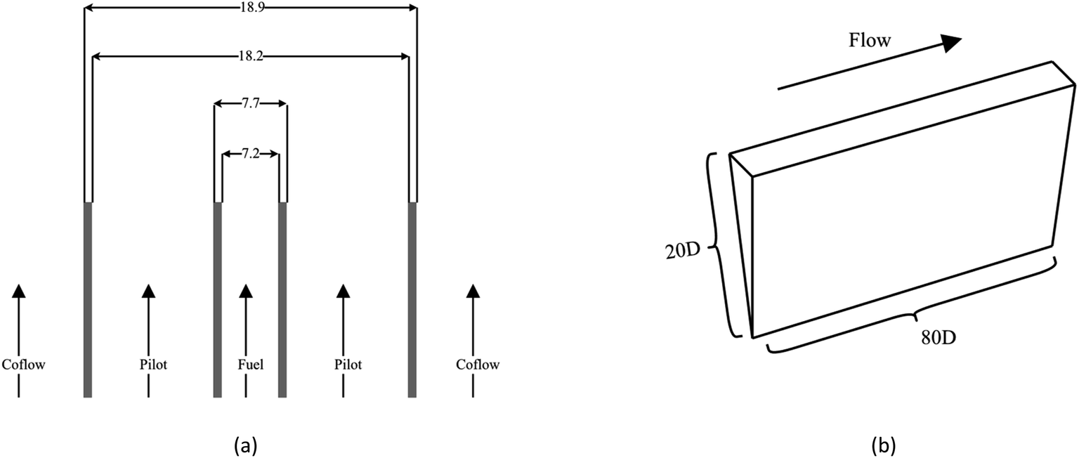 | ||
| Fig. 1 The burner schematic in cross section view (a) and axis view (b) of the Sandia Flame D. | ||
On the discretization of flamelet library, the mixture fraction and normalized progress variables have 101 uniform levels, and 11 points are used for the discretization of the variance of mixture fraction, which is further refined around the 0. Finally, the flamelet library resolution is set to  points and a 4-order linear-interpolation is used when this library get coupled with the CFD solver.
3. Results and discussion
3.1. Pre-processing for non-adiabatic flamelet library
Flamelet-like methods share a basic idea that the local turbulent flame can be identified as a set of one-dimensional flames. In other words, the multi-dimensional turbulent flame can be viewed as a series of one-dimensional laminar flames embedded in turbulent flow. Based on this assumption, two one-dimensional laminar flame are solved by FlameMaster34 with the unity Lewis number assumption (equal diffusivities for temperature and all species). The CD flame depends on the stoichiometric scalar dissipation rate χst. Therefore, a series of CD flame are solved to generate the CD flamelet library. Fig. 2a shows the maximum temperature (Tmax) in the one-dimensional flame solution as a function of the χst. Here, the upper half of the curve represents the steady-state flamelet solutions and the lower half of the curve represents the unsteady flamelet solutions. The stoichiometric scalar dissipation rate χst in each flamelet calculation is given manually. The UP flame solution depends on the composition of the initial mixture, and then it is generated by solving the laminar steady UP flames under different ratios of fuel and oxidizer. Fig. 2b gives the Tmax in the UP flame solution as a function of the mixture fraction. The thermochemical solutions beyond the flammability limit of laminar UP flames are obtained by extrapolation. These methods of generating flamelet library has received good feedback in many studies.37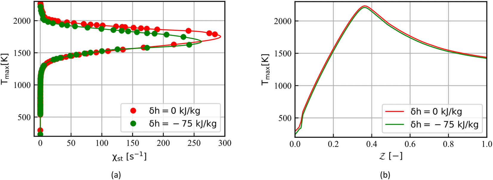 | ||
| Fig. 2 The distributions of Tmax in CD flamelets (a) and in UP flamelets (b). | ||
In Section 2.3, we propose a method to reduce the absolute enthalpy of the boundary to get the non-adiabatic flamelet solutions. Since the predicted temperature is closely related to NOx emissions, a maximum temperature analysis is performed firstly for two libraries. Fig. 2 shows the maximum temperature of each flamelet for a set of boundary conditions with enthalpy loss of 0 kJ kg−1 and −75 kJ kg−1. As shown in Fig. 2a, the temperature loss of CD flamelets increases with the χst growing up. However, a uniform drop of the maximum temperature in the UP flamelet solutions is observed in Fig. 2b. Based on the definition of absolute enthalpy and the given boundary conditions, an enthalpy loss of −75 kJ kg−1 is expected to reduce the temperature in Flame D simulation by about 50 K. This indicates that the CD flame solutions overestimate heat losses in the non-adiabatic flamelets generation.
As shown in Fig. 3, the inlet temperature of the laminar flame does not conform to the physical reality with the enthalpy loss treatment at the boundary. Fig. 3a shows the temperature of the CD flamelets as a function of the mixture fraction, the stoichiometric scalar dissipation rate is taken as 4.5. It can be seen that the temperature of the fuel side  and the oxidant side
  has a local temperature drop with the enthalpy loss −75 kJ kg−1, the fuel side is lower than 294 K and the oxidant side is lower than 291 K. In Fig. 3b, the initial mixture of the UP flame is taken as the mixture fraction 0.35 and the temperature as a function of the normalized reaction progress variable. Similarly, the temperature at the initial side
  is lower than 291 K with the enthalpy loss −75 kJ kg−1. Many thermochemical parameters are temperature dependent, such as species mass fractions, chemical reaction source term, and especially for NOx emission. Thus, this part of the solution that does not conform to physical reality requires special treatment. In the following, two steps are taken to generate the corrected non-adiabatic CD flamelet profile:37
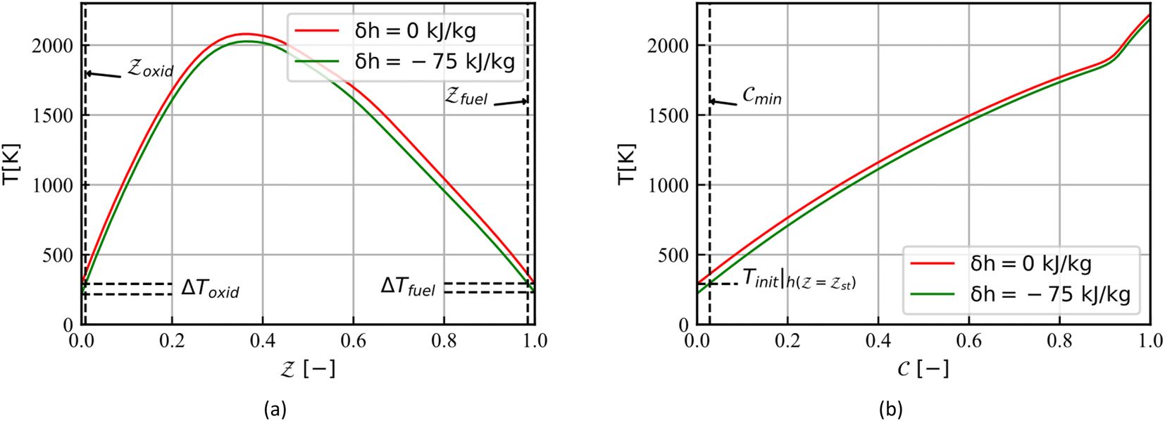 | ||
Fig. 3 Temperature profiles for CD flamelet with χst = 4.5 (a), and for UP flamelet with  (b). (b). | ||
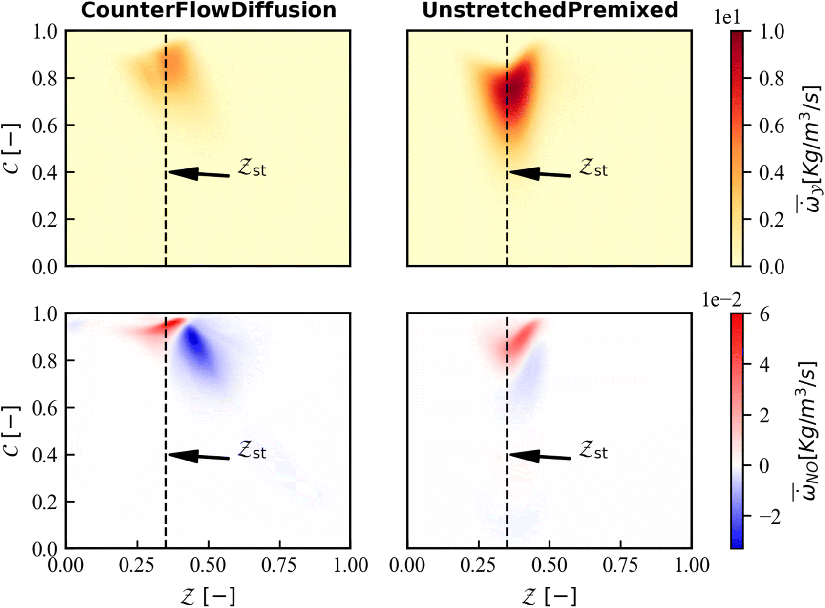 | ||
Fig. 4 Scatter point representation in  space. space. | ||
(i) Delete the parts of solution that has non-physical temperature;
(ii) Correct the mixture fraction range from [0–1] to  for presumed PDF integration.
Similarly, correct the normalized process variables range from [0–1] to  for non-adiabatic UP library. This treatment has a very negligible effect on simulation results.37
Two libraries applied in simulations are obtained with above mentioned special processing method. As shown in Fig. 4, the reaction progress variable source and the NO source that are used for CFD calculation are compared in the  space, where the enthalpy loss is 0 kJ kg−1. Compared with the UP flame, the NO sources in the CD library are more widely distributed and closer to the steady state reaction region
  . The explanation for this is that the CD flame with stretching effect underestimates the progress variable source and overestimates the NO source.
3.2. Effects of flamelet library on flame structure
In this section, the mean temperature and mean mass fraction of CO2, H2O and NO measured at the axis and at various axial positions are compared with the steady state numerical results to evaluate the effect of different laminar flamelet libraries on combustion simulations. The screenshots of steady temperature and the mass fraction of NO at the mid-plane of the domain give clear flame structure. Unlike the mass fraction of NO that is updated by an additional transport equation, steady state products such as CO2 and H2O are look-up directly from the libraries.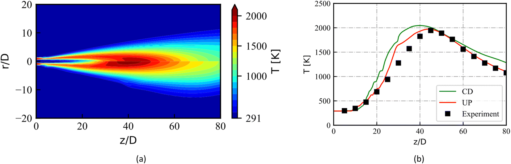 | ||
| Fig. 5 (a) The temperature distribution obtained from numerical simulation based on the two libraries. The upper part is from UP library and the lower part is from CD library. (b) The temperature profiles on the central axis. Red line marks UP library, green line marks CD library. | ||
The radial mean temperature plots at the z/D locations of 3, 15, 30, 45, 60 and 75 are shown in Fig. 6. These locations include the entire flow field, especially the last four points are where the main flame structure exists, which can better indicate the performance of the combustion model. Simulation results are compared with experimental data. At the location of z/D = 3, both the flamelet libraries predict well. They also give temperature distributions in agreement with experimental values at the locations of z/D = 15 and z/D = 45. However, the simulation temperature is higher than the experimental data at the locations of z/D = 30 for 0 ≤ r/D ≤ 2, especially the overestimation of the CD library is more serious. Errors can be reduced by choosing other turbulence and combustion models, but this is beyond the purpose of the present work. At positions of z/D = 60 and z/D = 75, the CD-based simulation results are higher than the UP-based results in the entire radial direction. Overall, these radial data support the conclusion that the UP library predict better temperature profiles.
 | ||
| Fig. 6 Radial profiles of temperature at six different locations along the axis. | ||
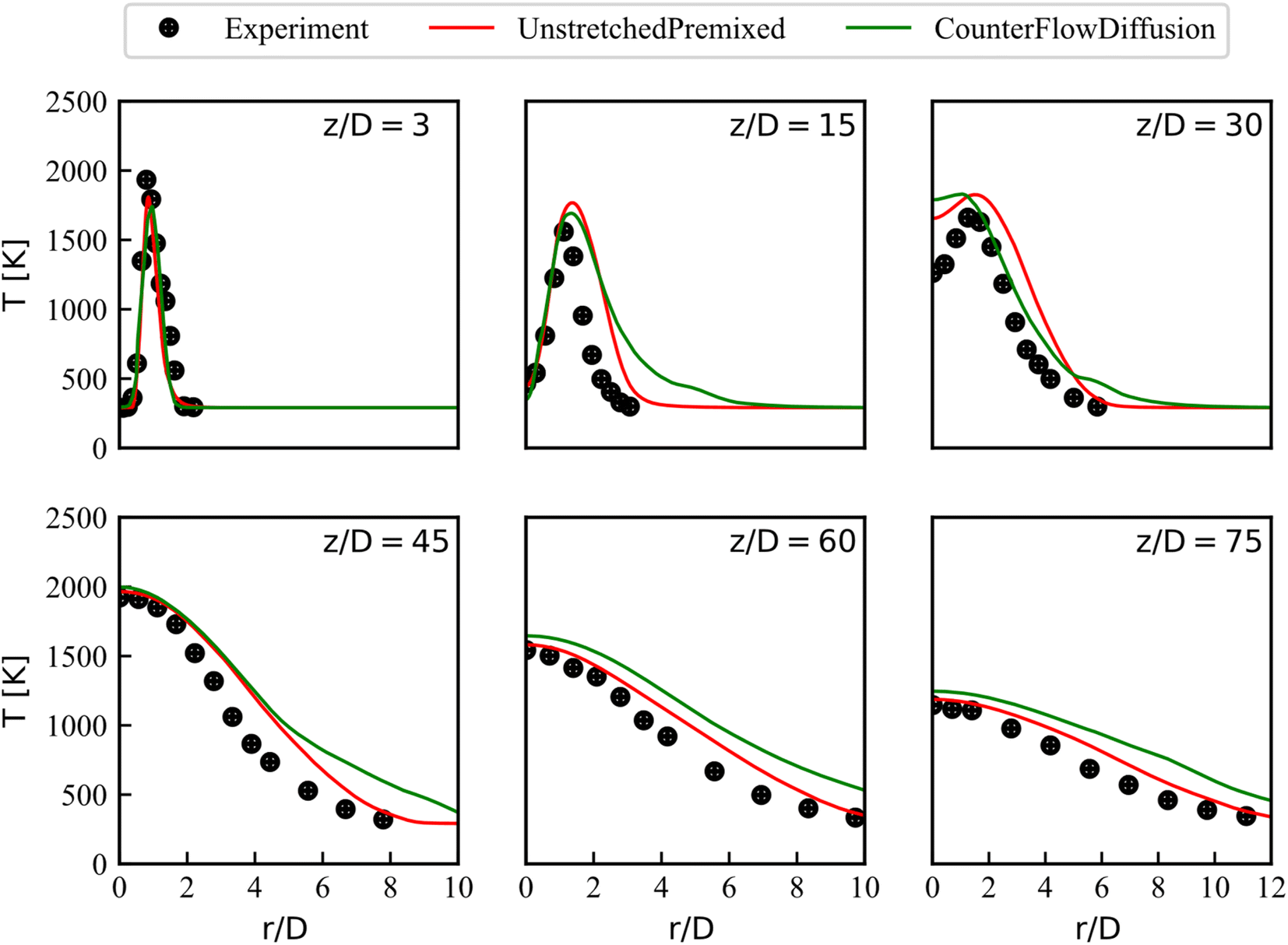
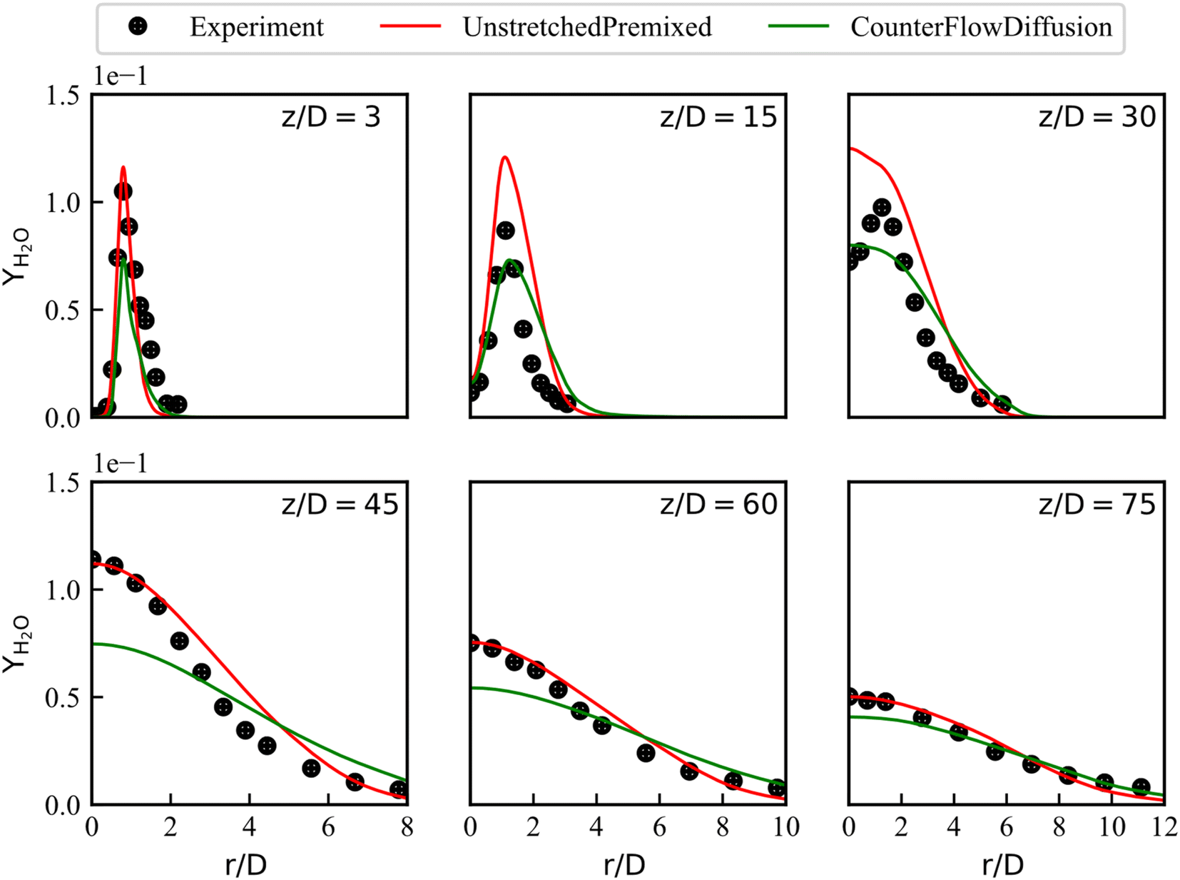
The radial mean mass fractions of CO2, H2O are compared with the experiments in Fig. 7 and 8, respectively. The numerical results of steady state products obtained from the UP library matched the experimental values well at all locations except at location of z/D = 30, where the mass fraction of H2O is overestimated, especially around r/D = 2. The larger errors in radial profiles of temperature and H2O are mainly manifested at location of z/D = 30 close to the central axis. The reasons for these errors are different. The overestimated temperature can be explained that the turbulence model underestimates the penetration distance of the scalar field, causing the high temperature zone to be closer to the upstream. But the global temperature profile trend is consistent with the experimental data. However, for the H2O profile at the same location in Fig. 7, the trend is inconsistent with the experimental data.
 | ||
| Fig. 7 Radial profiles of mass fraction of H2O at six different locations along the axis. | ||
 | ||
| Fig. 8 Radial profiles of mass fraction of CO2 at six different locations along the axis. | ||
Fig. 7 shows that it is difficult to capture the peak of H2O concentration distribution near the central axis at z/D = 30. This phenomenon should be analyzed together with Fig. 8 (the distribution of CO2 concentration) and the definition of progress variable (eqn (12)) that includes CO2 and not includes H2O. Therefore, the progress variable field obtained by the transport equation can well reproduce the distribution of CO2, such as the good agreement between UP predicted CO2 and experimental data, as shown in Fig. 8. In contrast, the mass fractions of species interpolated by the library, such as H2O, cannot reproduce the experimental peaks in some local flow fields, which is the reason for the additional transport equation of NO mass fraction.
With the CD library, the simulation results underestimate the mass fraction of H2O at the peak, while systematically overestimating the mass fraction of CO2 in the radical direction. In general, URANS coupled with the UP library are feasible method for pilot jet combustion modeling.
 ), respectively. The mean YNO obtained from the two libraries are very close in the upstream of the fuel jet (z/D < 15). The distribution of
  shows a large difference in shear layer, where represent regions of high scalar dissipation rates. The noticeable difference starts at the end of jet (z/D > 30), where the maximum value of YNO in the CD library is overestimated and has a wider distribution. Notably, the maximum value of
  in the CD library (Fig. 9b) is only 10% larger than that in the UP library, but four times larger in YNO (Fig. 9a). The distributions of YNO on the central axis are shown in Fig. 9c. The two distributions of YNO on the centerline are close to each other at the beginning of the jet (z/D < 25). However, the prediction of YNO of the UP library are much better where NOx emissions start to rise (z/D > 30).
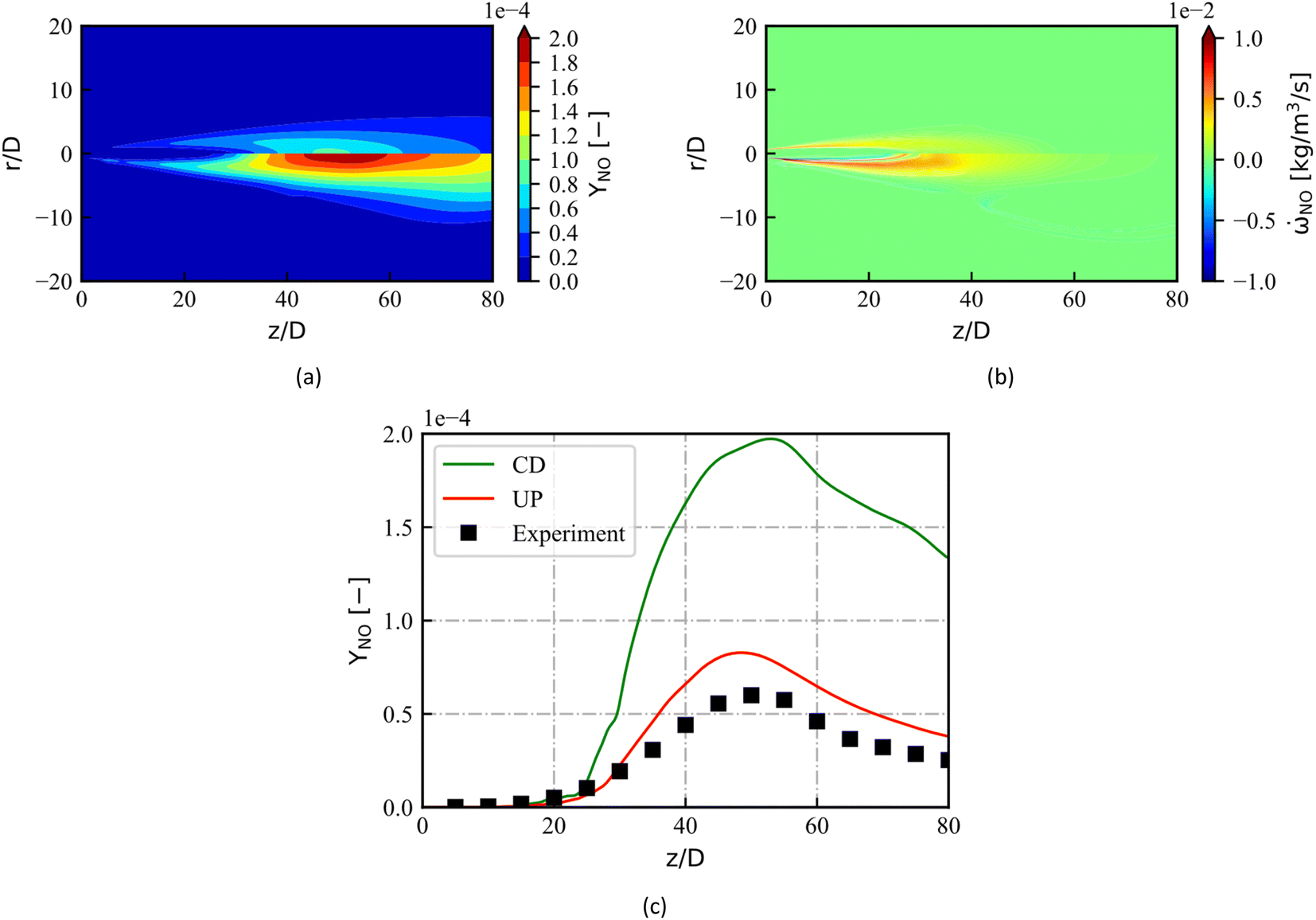 | ||
| Fig. 9 (a) The distribution of the mass fraction of NO, the upper part is from UP library and the lower part is from CD library. (b) The distributions of the NO source. (c) The NO profiles on the central axis, red line marks UP library, green line marks CD library. | ||
The experimental data of YNO are available at the axial locations of z/D = 3, 15, 30, 45, 60 and 75, they are compared with the numerical profiles of YNO in Fig. 10. The simulated YNO with the CD library significantly overestimated NO emissions at locations of z/D ≥ 30. Overall, the contours and centerline sampling of the mean YNO with UP library are consistent with experimental results. Compared with the 4.2 times overestimation of the maximum error in CD prediction of NO mass fraction, the UP prediction accuracy improved to 0.5 times overestimation referring to the experimental data. Details are shown in Table S1 and Fig. S2† in the ESI.†
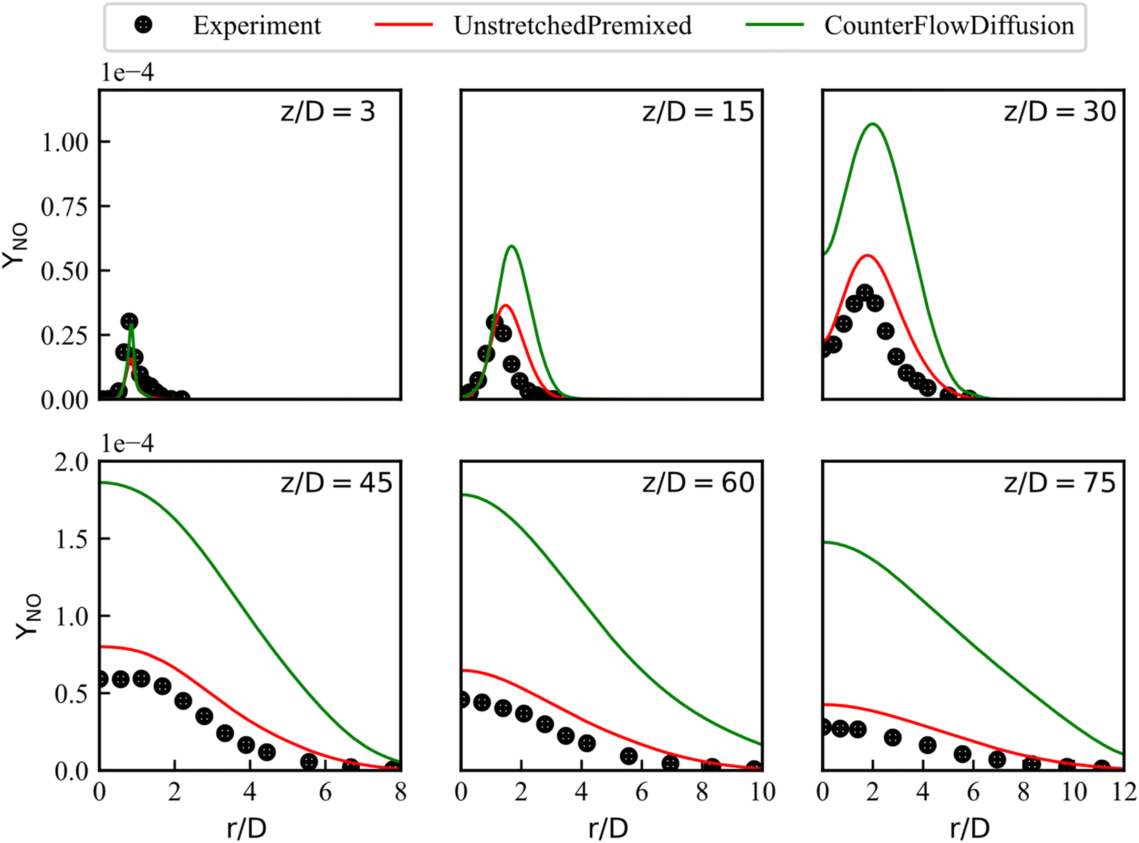 | ||
| Fig. 10 Radial profiles of mass fraction of NO at six different locations along the axis. | ||
The differences in YNO predictions are mainly attributed to the differences in  predictions. The RANS simulation results coupled CD library overestimate the temperature when z/D = 20–40. Considering the thermal NO mechanism, high temperature causes the NO source term increase, as shown in Fig. 5 and 9. Moreover, the actual combustion of the Sandia Flame D is complicated. As a pilot flame, there are both diffusion combustion and partial premixed combustion, as well as premixed combustion mode. In the high temperature region of Flame D, the actual NOX chemistry mainly dominated by the premixed combustion mode, so UP library gives a better estimation of NOX.
Analysis of the distribution of YNO shows that the library that is generated by the method of converting laminar CD flamelets with different stoichiometric scalar dissipation rates into  space has drawback on the prediction of NOx emissions. The UP library is a better modeling choice for accurate prediction of slow reaction product which are dominated by chemistry.
4. Conclusions
The numerical investigation of a turbulent pilot jet flame (Sandia Flame D) is carried out by developing a custom URANS solver in present study. The turbulence model adopts the standard k–ε model, and the combustion model adopts the flamelet chemistry tabulation method to avoid expensive chemical reaction integration costs. The absolute enthalpy and the mass fraction of species are obtained by interpolation from the library. To improve the prediction accuracy, the mass fraction of NO is solved by an additional transport equation. Two 4D non-adiabatic flamelet libraries are generated from the 1D laminar UP flame and the 1D laminar CD flame, respectively. Compared with the experimental data, the influence of the flamelet databases generated by different types of flamelets on the simulation results are discussed.The simulation results show that the NO field depends on the laminar flamelet type. Two 4D flame libraries provided almost the same range of values in terms of temperature and major species fields. The NO source term  in UP library introduces a reasonable agreement with measurement data by solving an additional NO transport equation. However, the 1D laminar CD flamelet solutions with detailed chemical mechanism introduces a larger value of
  and over-predicted YNO in simulations. Overall, URANS simulations based on the non-adiabatic 4D library of UP flamelet and the standard k–ε turbulence model can provide a high-precision prediction of NOx emission. The current study clearly demonstrates the feasibility of predicting NOx emissions using tabulated chemistry methods, and the unpredictable NOx emissions are numerically reproduced through a non-adiabatic library based on UP flames. The proposed method can be applied to high-precision numerical simulation of NOx emission for other engineering combustors.
Conflicts of interest
There are no conflicts to declare.Acknowledgements
This work is supported by the National Natural Science Foundation of China (No. 91741201).References
- S. Iavarone and A. Parente, Front. Mech. Eng., 2020, 6, 13 CrossRef.
- M. Ravikanti, M. Hossain and W. Malalasekera, Proc. Inst. Mech. Eng., Part A, 2009, 223, 41–54 CrossRef CAS.
- T. Lu and C. K. Law, Prog. Energy Combust. Sci., 2009, 35, 192–215 CrossRef CAS.
- H. Xue and S. K. Aggarwal, Combust. Flame, 2003, 132, 723–741 CrossRef CAS.
- H. Guo and G. J. Smallwood, Int. J. Therm. Sci., 2007, 46, 936–943 CrossRef CAS.
- V. Fichet, M. Kanniche, P. Plion and O. Gicquel, Fuel, 2010, 89, 2202–2210 CrossRef CAS.
- M. Zhang, Z. Fu, Y. Lin and J. Li, Chin. J. Aeronaut., 2012, 25, 854–863 CrossRef CAS.
- Y. Kang, Q. Wang, X. Lu, H. Wan, X. Ji, H. Wang, Q. Guo, J. Yan and J. Zhou, Appl. Energy, 2015, 149, 204–224 CrossRef CAS.
- A. Innocenti, A. Andreini, D. Bertini, B. Facchini and M. Motta, Fuel, 2018, 215, 853–864 CrossRef CAS.
- S. Iavarone, M. Cafiero, M. Ferrarotti, F. Contino and A. Parente, Int. J. Hydrogen Energy, 2019, 44, 23436–23457 CrossRef CAS.
- E. C. Okafor, K. D. K. A. Somarathne, R. Ratthanan, A. Hayakawa, T. Kudo, O. Kurata, N. Iki, T. Tsujimura, H. Furutani and H. Kobayashi, Combust. Flame, 2020, 211, 406–416 CrossRef CAS.
- C. Schluckner, C. Gaber, M. Landfahrer, M. Demuth and C. Hochenauer, Fuel, 2020, 264, 116841 CrossRef CAS.
- A. B. Wakale, S. Banerjee and R. Banerjee, J. Energy Inst., 2020, 93, 1868–1882 CrossRef CAS.
- M. Sripathi, S. Krishnaswami, A. M. Danis and S.-Y. Hsieh, in Turbo Expo: Power for Land, Sea, and Air, American Society of Mechanical Engineers, 2014, vol. 45691, p. V04BT04A060 Search PubMed.
- R. Saini, S. Prakash, A. De and R. Yadav, Therm. Sci. Eng. Prog., 2018, 5, 144–157 CrossRef.
- A. C. Zambon, B. Muralidharan, A. Hosangadi and K. Ajmani, in AIAA Propulsion and Energy 2020 Forum, American Institute of Aeronautics and Astronautics, 2020 Search PubMed.
- O. Gicquel, N. Darabiha and D. Thévenin, Proc. Combust. Inst., 2000, 28, 1901–1908 CrossRef CAS.
- N. Peters, Prog. Energy Combust. Sci., 1984, 10, 319–339 CrossRef CAS.
- C. D. Pierce and P. Moin, J. Fluid Mech., 2004, 504, 73–97 CrossRef CAS.
- J. A. van Oijen, A. Donini, R. J. M. Bastiaans, J. H. M. ten Thije Boonkkamp and L. P. H. de Goey, Prog. Energy Combust. Sci., 2016, 57, 30–74 CrossRef.
- J. A. V. Oijen and L. P. H. D. Goey, Combust. Sci. Technol., 2000, 161, 113–137 CrossRef.
- G. Godel, P. Domingo and L. Vervisch, Proc. Combust. Inst., 2009, 32, 1555–1561 CrossRef CAS.
- v. J. A. Oijen and d. L. P. H. Goey, Proceedings of the European Combustion Meeting, 2009 Search PubMed.
- M. Ihme and H. Pitsch, Phys. Fluids, 2008, 20, 055110 CrossRef.
- H. Yigit Akargun, B. Akkurt, N. G. Deen and L. M. T. Somers, in The Proceedings of the International symposium on diagnostics and modeling of combustion in internal combustion engines, The Japan Society of Mechanical Engineers, 2017, p. A105 Search PubMed.
- J. Tang and W. Song, J. Propul. Technol., 2017, 38, 1523–1531 CAS.
- Q. Yao, Y. Zhang, X. Wang, Z. Tian, G. Hu and W. Du, Neurocomputing, 2022, 482, 224–235 CrossRef.
- Z. An, M. Zhang, W. Zhang, R. Mao, X. Wei, J. Wang, Z. Huang and H. Tan, Fuel, 2021, 304, 121370 CrossRef CAS.
- W. Zhang, S. Karaca, J. Wang, Z. Huang and J. van Oijen, Combust. Flame, 2021, 227, 106–119 CrossRef CAS.
- H. Jasak, PhD thesis, Imperial College London (University of London), 1996 Search PubMed.
- H. G. Weller, G. Tabor, H. Jasak and C. Fureby, Comput. Phys., 1998, 12, 620 CrossRef.
- W. P. Jones and B. E. Launder, Int. J. Heat Mass Transfer, 1972, 15, 301–314 CrossRef.
- W. L. Grosshandler, RADCAL: A Narrow-Band Model for Radiation Calculations in a Combustion Environment, 1993 Search PubMed.
- P. J. Coelho, O. J. Teerling and D. Roekaerts, Combust. Flame, 2003, 133, 75–91 CrossRef CAS.
- H. Pitsch, FlameMaster, A C++ Computer Program for 0D Combustion and 1D Laminar Flame Calculations Search PubMed.
- R. W. Bilger, Combust. Sci. Technol., 1976, 13, 155–170 CrossRef.
- S. K. Sadasivuni, LES Modelling of Non-premixed and Partially Premixed Turbulent Flames, Loughborough University, 2009 Search PubMed.
- T. Li, F. Kong, B. Xu and X. Wang, Appl. Math. Mech., 2019, 40, 1197–1210 CrossRef.
- C. T. Bowman, R. K. Hanson, D. F. Davidson, W. C. Gardiner Jr, V. Lissianski, G. P. Smith, D. M. Golden, M. Frenklach and M. Goldenberg, GRI-Mech 2.11, http://www.me.berkeley.edu/gri_mech/ Search PubMed.
- R. V. Murthy, Advanced Flamelet Modelling of Turbulent Nonpremixed and Partialy Premixed Combustion, Loughborough University, 2008 Search PubMed.
- G. P. Smith, D. M. Golden, M. Frenklach, N. W. Moriarty, B. Eiteneer, M. Goldenberg, C. T. Bowman, R. K. Hanson, S. Song, W. C. Gardiner Jr, V. V. Lissianski and Z. Qin, GRI-Mech 3.0, http://www.me.berkeley.edu/gri_mech/ Search PubMed.
- R. Barlow, J. Frank, A. Karpetis and J. Chen, Combust. Flame, 2005, 143, 433–449 CrossRef CAS.
Footnote |
| † Electronic supplementary information (ESI) available. See DOI: https://doi.org/10.1039/d2ra06075b |
| This journal is © The Royal Society of Chemistry 2023 |