Automated analysis of transmission electron micrographs of metallic nanoparticles by machine learning

Abstract

Metallic nanoparticles were analysed with respect to size and shape by a machine learning approach. This involved a separation of particles from the background (segmentation), a separation of overlapping particles, and the identification of individual particles. An algorithm to separate overlapping particles, based on ultimate erosion of convex shapes (UECS), was implemented. Finally, particle properties like size, circularity, equivalent diameter, and Feret diameter were computed for each particle of the whole particle population. Thus, particle size distributions can be easily created based on the various parameters. However, strongly overlapping particles are difficult and sometimes impossible to separate because of an a priori unknown shape of a particle that is partially lying in the shadow of another particle. The program is able to extract information from a sequence of images of the same sample, thereby increasing the number of analysed nanoparticles to several thousands. The machine learning approach is well-suited to identify particles at only limited particle-to-background contrast as is demonstrated for ultrasmall gold nanoparticles (2 nm).

---

Introduction

Nanoparticles play a key role in materials science. As most nanoparticle properties depend on the particle size and size distribution, it is usually necessary to fully characterize a given set of particles. Many methods are available that give particle size distribution data, both in solid form (as powder) and in dispersed form.^1–6 However, shape-related parameters are usually only accessible by microscopic techniques. In that case, electron microscopy is the method of choice because light microscopy usually does not provide sufficient resolution.

For the application of nanoparticles and (nano-)fibres, e.g. in consumer products, cosmetics, drugs, or in heterogeneous catalysis, the particle shape plays a decisive role.^7–11 In occupational medicine and particle toxicology, rod-like (nano)particles are considered to be potentially more harmful, based on the case of asbestos where fibres cause strongly adverse effects upon inhalation.^12–14 Thus, nanoparticle populations are usually visualized by electron microscopy, followed by an extraction of their individual size- and shape-related properties.

A detailed analysis of electron micrographs of nanoparticles is often performed manually by human evaluators. This procedure is tedious, time-consuming, and inaccurate. It may also involve a considerable degree of human bias due to an unconscious selection of “typical” nanoparticles, e.g. particles with the “expected” size or the “desired” uniform shape. In the literature, claims of allegedly uniform nanoparticle populations after shape-specific syntheses, based on only a dozen depicted nanoparticles, are not uncommon.

Computational methods for detecting and analysing micrographs of nanoparticles do exist, however for many of them a considerable degree of manual input and fine-tuning of parameters is needed. Furthermore, many of these techniques fail for images with a low signal-to-noise ratio as it is the case for some high-resolution TEM images and images acquired with low beam intensity.^15,16

Clearly, an objective method for a rapid nanoparticle analysis from electron microscopic data is necessary. The rise of artificial intelligence/machine learning/deep learning has considerably enhanced our ability to train computers to recognize and autonomously analyse particles. Machine learning techniques have already been applied to electron microscopic images where they usually outperform classical image analysis approaches, especially when noisy images or overlapping particles are involved^15,17–25 (see ref. 26–28 for recent reviews). However, the reported approaches either do not extend to the analysis of bright-field high-resolution TEM images or are based on very small datasets, making them not generally applicable.

Here we present an automated method, based on machine learning, that permits to analyse electron microscopic images containing thousands of nanoparticles within a few seconds. This is based on previous training on suitable images. Typical parameters that can be extracted for each particle are size, circularity, equivalent diameter, and Feret diameter. These parameters are tedious to extract by manual examination, but readily available after the particles have been identified and their two-dimensional shape has been determined. If a high number of particles is analysed, the corresponding distribution functions, averages, and standard deviations can be easily computed. In addition, an algorithm to separate overlapping particles was implemented.

Thus, we have combined and adapted existing methods which have shown good results for other types of electron microscopic data to make them applicable to bright-field high-resolution TEM images. We demonstrate the capabilities of this method on a selection of images of metallic nanoparticles.

Results and discussion

We have implemented an autonomous pathway by which transmission electron microscopy (TEM) images of nanoparticles can be analysed in a fully automated way. This is based on the analysis of the TEM images to identify and extract individual particles, assisted by machine learning. The goal of the processing routine was to automatically extract shape- and size-related information of nanoparticles from TEM images. Fig. 1 summarizes the different steps in this routine. The routine was programmed in MATLAB.²⁹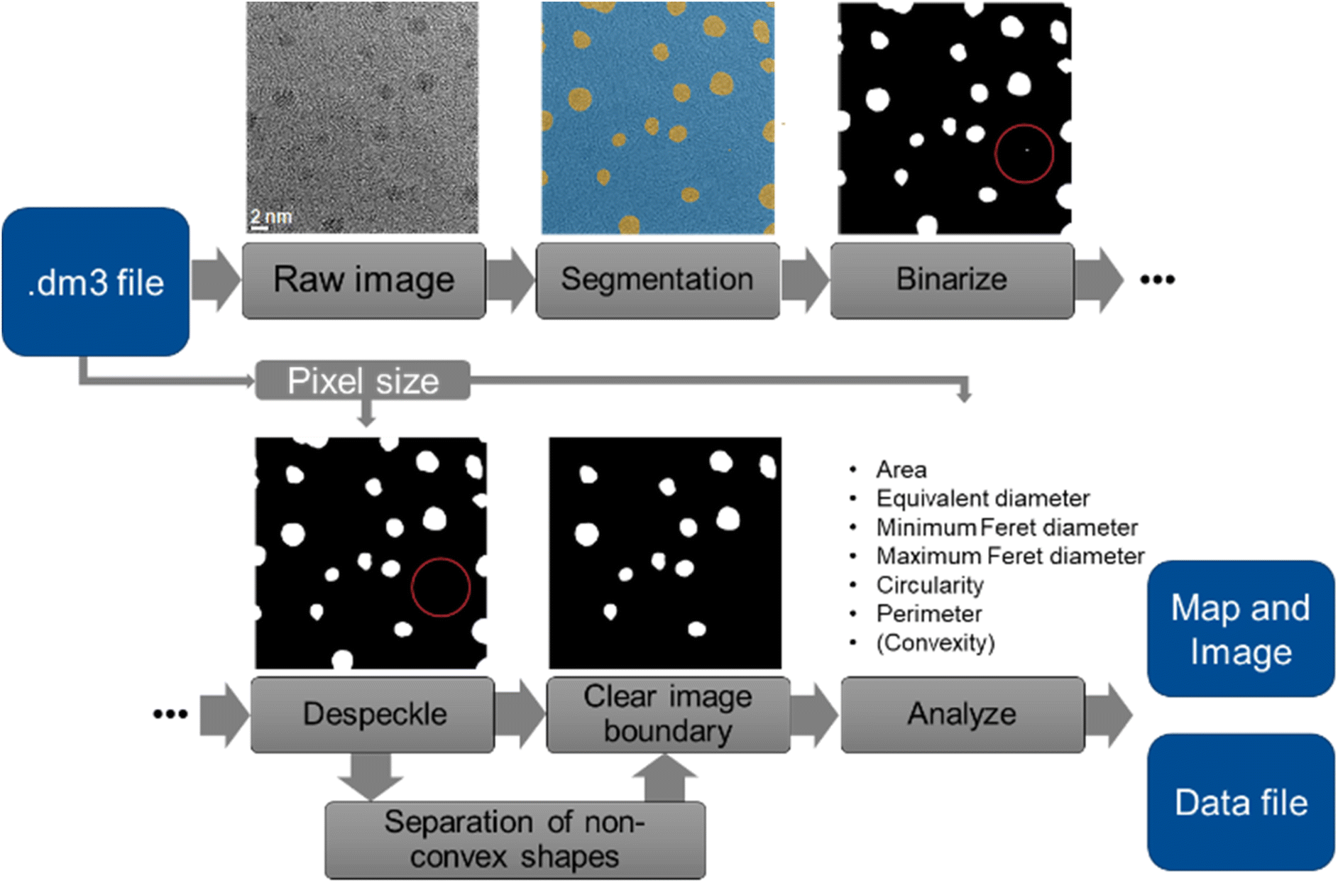

Fig. 1 Illustration of the TEM image processing routine. A typical speckle that was removed is labelled by a red circle.

First, the program loads the image and extracts its pixel size from the image file (dm3 format; DigitalMicrograph files from Gatan, Inc.) with a routine from MATLAB file exchange.³⁰ Next, the image is segmented by a trained neural network. From the resulting segmentation map, a binary particle segmentation map is created. The segmentation map is de-speckled to remove small mislabelled areas (“speckles”) from the map. Each area with an equivalent diameter below 0.5 nm is considered as a speckle and removed. Likewise, holes in particle areas with a diameter below 0.5 nm are closed. Particles that cross the image boundary are cropped by definition, therefore they cannot be evaluated. Consequently, they are generally removed from the particle map and excluded from further analysis. From the remaining particle-based areas, individual particles are identified and analysed for their shape and size. From the dimensions of each particle, we can compute its area, circular equivalent diameter (= diameter of the circle having the same area), minimum and maximum Feret diameter, perimeter, and circularity (circularity = 4 × area × π/perimeter²).

Two different options to deal with overlapping particles were implemented. This is important to avoid the misrepresentation of two overlapping particles as one single (and usually apparently distorted) particle, e.g. a peanut-shaped overlap of two spherical particles. Both options are based on measuring the convexity of particle regions as illustrated in Fig. 2. The convexity is defined as the ratio of the perimeter of the convex hull of a particle to the actual perimeter of a particle. Thus, a particle with concave indentations or an agglomerate of two sphere-like particles have a convexity < 1. Here, we considered particles with a convexity below 0.95 as non-convex and therefore consisting of overlapping particles, following the recent suggestion by Wang et al.³¹

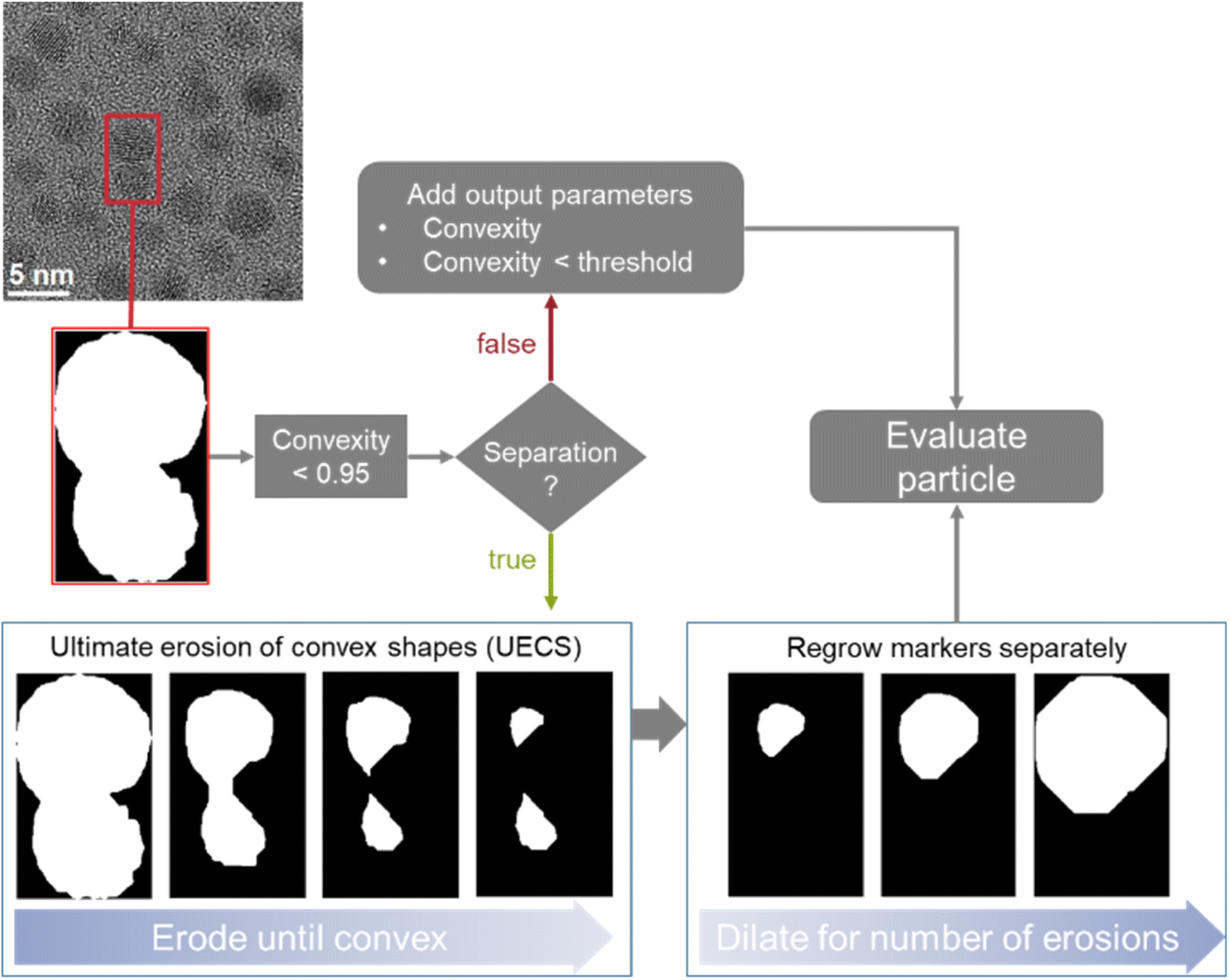Fig. 2 Illustration of the implemented options to deal with overlapping particles and illustration of the erosion and dilation process in particle separation.

In the first option, when no separation is used, convexity is added as an output parameter so that overlapping particles can be identified within the dataset. The program also labels all particles that are below the convexity threshold as such in the dataset. This option is useful if the number and size of agglomerates in a given sample are of interest.

The second option is to use dedicated algorithms to split overlapping particles. This was realized by an adaptation of the ultimate erosion of convex shapes (UECS) algorithm based on the description and MATLAB code by Park et al.^16,32 With this approach, particle regions are eroded until they exceed the convexity threshold. These eroded areas serve as markers for the singular particles which are then dilated back to their original size by dilating them for as many steps as they were previously eroded. The original outline is used as a mask to ensure that no additional pixels are labelled as particles. It is not combined with a watershed algorithm as that would not account for the overlapping area. If the particle is again non-convex after the regrowing procedure, it will be discarded and excluded from further analysis. If the markers reach an area below 30 pixels or are smaller than 0.5 nm in equivalent diameter before surpassing the convexity threshold, they are discarded. This option enables a fully automated processing of overlapping particles and is implemented as the default option. The limits of 30 pixels and/or 0.5 nm identified as suitable after analysing a number of images with the developed algorithm and visually inspecting the results for efficient particle separation.

After the completed analysis, all particle parameters are exported as xlsx or csv files. These also shows which particles resulted from the separation routine. TEM images and the segmentation maps are finally exported as png files. The program can process single image files (dm3 format) as well as stacks of image files. The results can be saved as individual evaluation datasets for each image or combined in one evaluation dataset.

In the following, we demonstrate the single evaluation steps with suitable examples. The separation of particles from the background is commonly denoted as segmentation. Representative data for a variety of metallic nanoparticles are shown in Fig. 3. The network is able to segment nanoparticles of different metals and sizes. Note that these images always depict metallic nanoparticles which have a high electron contrast, even if they are ultrasmall (1–2 nm). Usually, the segmentation becomes increasingly difficult if the contrast becomes weaker and if the nanoparticles become smaller. High-contrast images can often be segmented without the application of machine learning by standard image processing procedures (rendering, contrast variation), but the performance of image processing drops drastically for images with lower contrast or higher background noise. However, our machine learning approach showed the same performance for low-contrast images as with high-contrast images. This illustrates the advantage of the machine learning approach over conventional image processing.

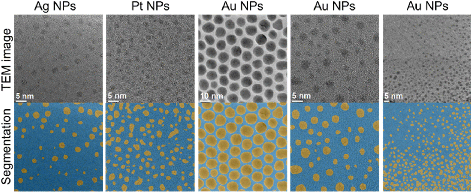Fig. 3 Representative examples of the separation of metallic nanoparticles from the background (segmentation).

A typical quantitative evaluation of ultrasmall gold nanoparticles of about 2 nm diameter is shown in Fig. 4. The particle map shows all particles that were included in the analysis. The particle size distribution is expressed by equivalent diameter (2.1 ± 0.7 nm), as well as minimum (2.0 ± 0.7 nm) and maximum Feret diameter (2.4 ± 0.8 nm). A manual evaluation by a human reviewer is also given (2.0 ± 0.5 nm) and shows good agreement with the automated evaluation.

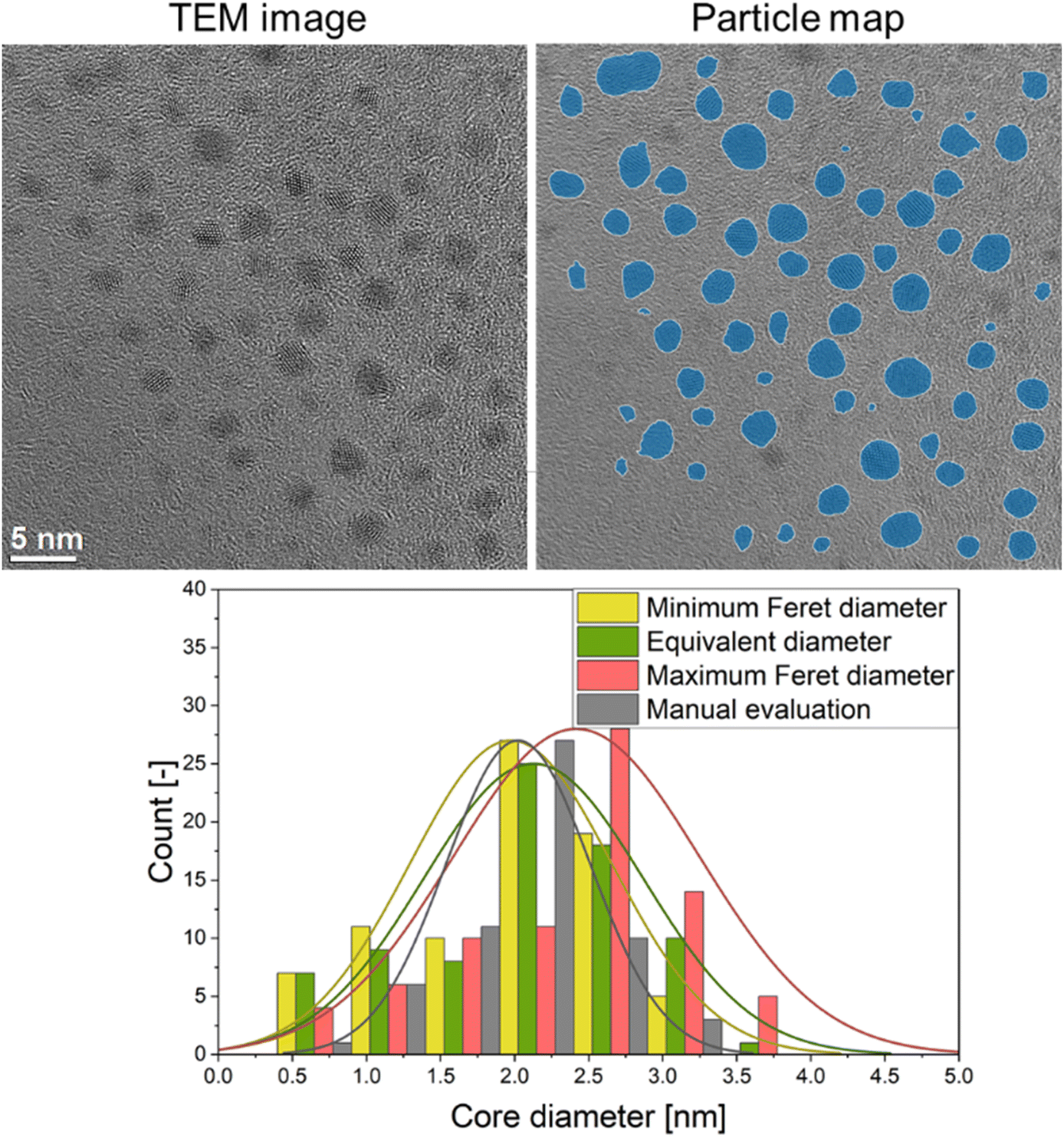Fig. 4 Particle size distribution results (minimum and maximum Feret diameters and equivalent diameter) obtained by the automated image processing routine of a TEM image of ultrasmall gold nanoparticles together with a manual determination of the distribution of the particle equivalent diameters by a human evaluator for comparison.

For a typical TEM image with a low degree of overlapping particles, this processing routine takes less than 15 seconds if the particle separation algorithm is used and less than 10 seconds if only the convexity is evaluated but no particle separation is performed. For images with higher degree of overlap, the program execution takes less than 90 seconds if particle separation is applied by iterative erosion and dilation. These durations refer to an execution of the program on the same machine that was used for training the neural network (see methods for details). This is a significant time improvement compared to a manual inspection which takes about 30 minutes for a typical image. It also enables an unbiased and quick analysis of large data quantities. An option to analyse multiple images from different regions of one given sample is also implemented. This increases the number of analysed particles and improves the particle statistics. An example of such an evaluation is shown in Fig. 5. The average equivalent diameter, its standard deviation, and the particle circularity were determined from 1465 particles, i.e. a high number. Note that the particle-to-background contrast in these images was limited because the nanoparticles were ultrasmall (about 2 nm). Thus, classical image analysis routines usually fail in this evaluation.

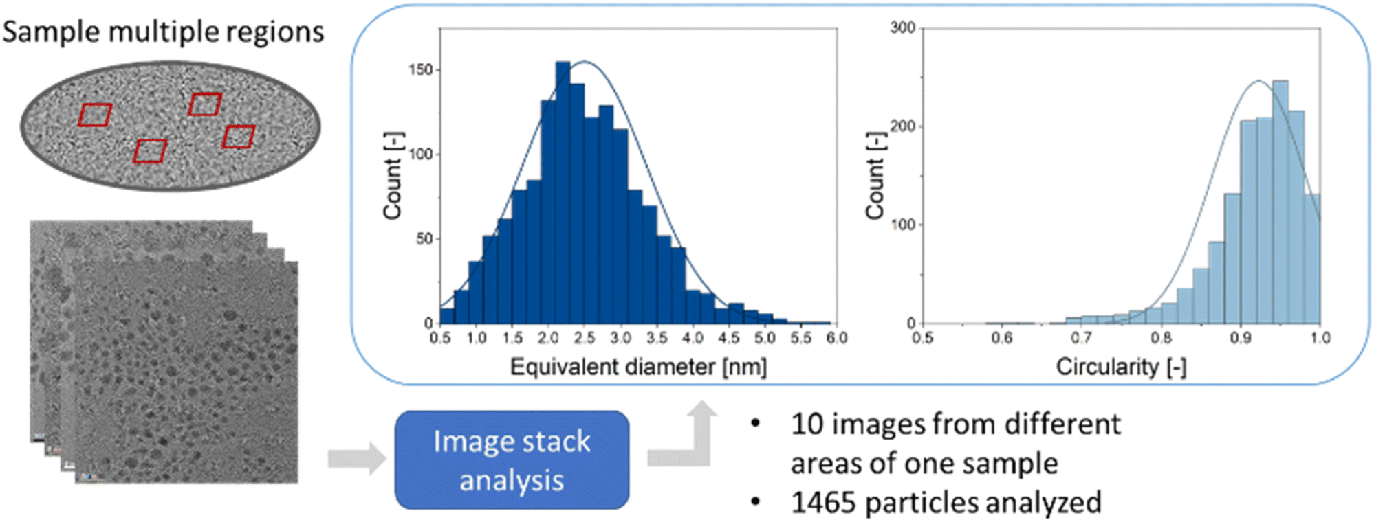Fig. 5 Example of an analysis of TEM images taken from multiple regions of one gold nanoparticle sample by the automated image processing routine and the accumulated results for equivalent diameter (2.5 ± 0.9 nm) and circularity (0.92 ± 0.06).

While the network was trained on spherical particles, it was also able to segment particles with other morphologies such as cubes or octahedra as shown in Fig. 6. For particles with a generic non-convex shape (Fig. 6, left image) the separation routine obviously cannot be used. In that case the program can only evaluate images with no overlapping particles.

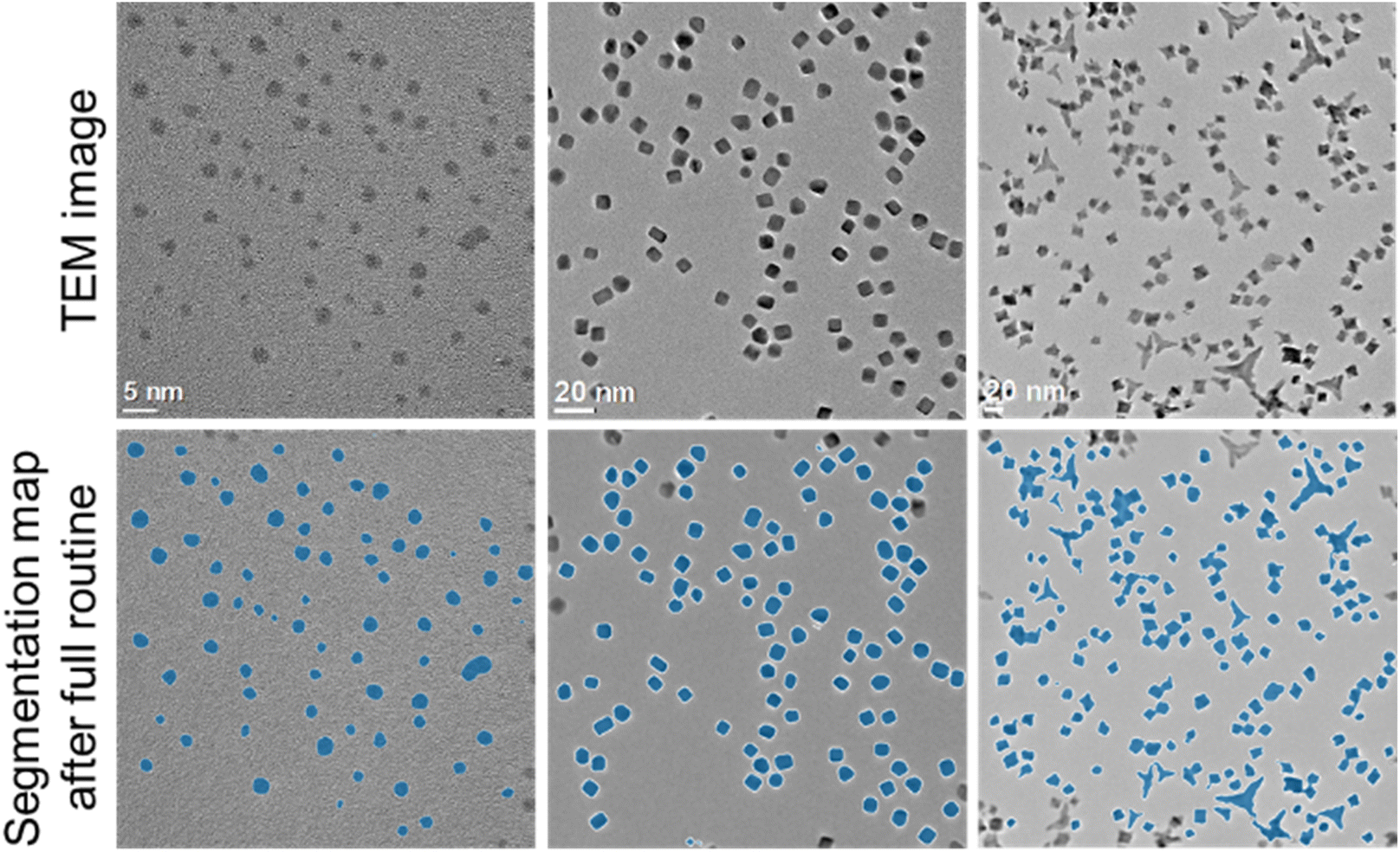Fig. 6 Analysis of TEM images with different shapes of gold (left) and platinum (centre and right) nanoparticles.

A limitation of the automated routine is the analysis of images with a high degree of particle overlap, as the particle separation routine used performs best for low to medium particle overlap.³²Fig. 7 shows typical images to illustrate the performance of the routine for different degrees of particle overlap. While most of the segmented particle regions are retained for all images, separation of particle regions with high degrees of overlap is more prone to errors and an overestimation of particle sizes.

Fig. 7 Examples of images of ultrasmall gold nanoparticles that can and cannot be properly evaluated due to different degrees of particle overlap. The segmentation image (middle) shows pixels in the foreground in yellow. The particle separation map (bottom) shows individually identified particles in blue.

Another limitation for particle separation comes with particles that overlap in such a way that they have a convexity which is high enough to pass the convexity exclusion criteria of a minimum convexity of 0.95. For some particles this can be solved by increasing the convexity threshold. However, this can also lead to the wrongful exclusion of particles with indentations. In principle, particles can also overlap in such a way that even a higher convexity threshold would not lead to a successful separation. An example would be an ellipse resulting from two closely overlapping spheres. These particles are then counted as one even after the separation algorithm. We found that not much can be done against this problem.

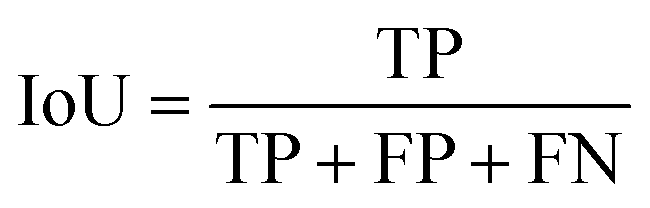
The overall performance of a trained neural network is generally expressed by accuracy, intersection over union (IoU), and DICE coefficient.^33,34 These metrics can be given as global or class-based metrics. The global accuracy describes the amount of correctly classified pixels given as true negatives (TN) and true positives (TP) in relation to the overall number of pixels which includes the false positives (FP) and false negatives (FN). The class-based accuracy does not include TN and FP.

IoU is defined as the amount of overlap between the ground truth and the segmentation map divided by their union. With respect to true and false positive and negative values, IoU is defined as follows:

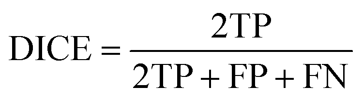
The DICE coefficient is calculated as the union between the ground truth and the segmentation map weighed by factor two and then divided by the sum of the man and the segmentation map.

The network reached a final validation accuracy of 96.14% during training. All further performance metrics were calculated based on the test dataset. The global accuracy of the test dataset was 96.26% and therefore comparable with the validation accuracy. As the classes were unbalanced with around 80% of all pixels in the images being background, it is important to look into other metrics besides the global accuracy. Fig. 8 shows the class accuracy as a normalized confusion matrix with the particle class showing a similar value to the global accuracy of 96.12%. Table 1 shows the IoU and DICE coefficient for the test dataset. Both have values above 80% for the particle class and values above 95% for the background class, i.e. the programmed routine performed very efficiently. It outperformed other machine learning based approaches for analysing similar TEM images.¹⁵

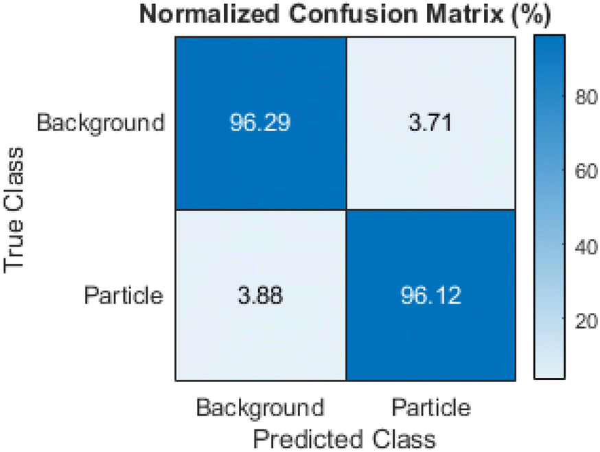Fig. 8 Normalized confusion matrix for the trained network on the test dataset, showing the percentage of pixels in a given class in the ground truth (true class) being allocated to different classes by the network (predicted class).

Table 1 Intersection over union score (IoU) and DICE coefficient of the trained network on the test dataset

	IoU/%	DICE coefficient/%
Background	95.42	97.67
Particle	83.00	90.71

---

Experimental

Methods

Electron microscopy. High-resolution transmission electron microscopy (TEM) was performed with an aberration-corrected FEI Titan transmission electron microscope equipped with a Cs-probe corrector (CEOS Company), operating at 300 kV.³⁵ The nanoparticle dispersion was drop-cast on a copper grid, and coated with an ultrathin amorphous carbon film. Representative TEM images of metallic nanoparticles were used for training and analysis.

Machine learning. A deeplabv3+ network with a resnet-18 backbone was trained on TEM images to distinguish between nanoparticles and the background by semantic segmentation with a supervised learning approach.^36,37 The training was performed on 128 manually labelled TEM images of a wide variety of nanoparticle samples of different metals and sizes. The dataset included images of ultrasmall nanoparticles that were in the size range of 1 to 10 nm. Manual particle labelling and the determination of the equivalent particle diameters were performed by experienced human evaluators.

Labelling was performed with MATLAB's image labeller tool.³⁸ Training was performed in MATLAB with a deeplabv3+ network with a pretrained resnet-18 network as a backbone that is available from Mathworks^36,39 (see, e.g., ref. 28 and 40 for general discussions on the application of CNNs in particle analysis in electron microscopy). As good results were obtained with these CNNs, other CNNs were not tested. The full TEM images had a size of either 2048 × 2048 pixels or 1024 × 1024 pixels. To speed up training with only a small loss in image resolution, the images and ground truth images (labels) were sized down to an image size of 1024 × 1024 pixels and then sliced into 256 × 256 pixel tiles which were then used for training. Additionally, the full image was also included in the training data by reducing it to a 256 × 256 pixel image. This resulted in 2176 labelled image slices. The manually labelled images were split into a training, a validation and a test dataset, respectively, in a ratio of 60 : 20 : 20. To enhance training by more variety in the images, data augmentation was applied with scaling, rotation, x- and y-axis reflection, brightness and contrast augmentation of the individual images. The validation loss and accuracy were checked every other epoch during training to monitor for overfitting.

The semantic segmentation training was performed on a Dell Precision 7920 Tower equipped with an NVIDIA Quadro RTX 5000. It was equipped with 32 GB RAM and an Intel® Xeon® Gold 6226R Processor. Training was performed for 120 epochs with a batch size of 30 and an initial learning rate of 0.01. The learning rate was decreased every 15 epochs by a learning rate drop factor of 0.75.

The network performance was analysed by global and class accuracy, intersection over union score (IoU) and DICE score (also known as F1 score).^33,34

The code for the described procedures, denoted here with the acronym ANTEMA, including reference images, is available on GitHub at https://github.com/ngumb/ANTEMA.

Conclusions

A machine learning approach for TEM data analysis creates more accurate and user-independent results and avoids human bias. High numbers of nanoparticles can be extracted from TEM images and automatically analysed. The presented automated analysis is significantly faster than a manual evaluation and allows the analysis of multiple images of one sample. This leads to more nanoparticles being analysed and a better statistical accuracy. Furthermore, the algorithm extracts multiple parameters for each particle, thus yielding more data about a particle than just the average core diameter. This routine and the trained neural network can also be used to analyse large datasets like in situ datasets. We conclude that the application of machine learning techniques to two-dimensional TEM images, even with poor contrast, can considerably improve the statistical basis to characterize nanoparticle samples with respect to size and shape.

As a general limitation of the analysis of TEM images, it must be emphasized that particles are almost always represented as two-dimensional projections in microscopy. Neither human trainers nor artificial intelligence are able to reconstruct data which are not known. For instance, the two-dimensional depiction of a circular particle is usually tacitly (and often unconsciously) transformed into a three-dimensional sphere. The fact that this circle could also be the two-dimensional projection of a circular platelet, a cylinder, or a disc-like object is often not considered. If all circular discs lay flat on the sample holder, they would also give a circular projection. Three-dimensional shape information can only be gained if particles are imaged from different orientations. Tomography would be the method of choice. However, as this is time-consuming, it is usually applied only to individual particles. It is not possible to apply this method to very small nanoparticles on the ultrasmall length scale (1–2 nm). Thus, there is still a long way to go until we can assign particle populations to their full three-dimensional properties. For now, the presented routine is a powerful tool for an automated analysis of two-dimensional TEM images of nanoparticles.

Author contributions

Conceptualization: M. E. and N. G.; methodology: M. E. and N. G.; investigation: N. G., K. L. and M. H.; programming: N. G.; visualization: N. G.; validation: all authors; writing—original draft preparation: M. E. and N. G.; writing—review: all authors. All authors have read and agreed to the published version of the manuscript.

Conflicts of interest

There are no conflicts to declare.

Acknowledgements

M. E. and M. H. are grateful to the Deutsche Forschungsgemeinschaft (DFG) for generous funding in the projects EP 22/62-1 and HE 7192/8-1. We acknowledge support by the Open Access Publication Fund of the University of Duisburg-Essen.

Notes and references

1. F. Caputo, J. Clogston, L. Calzolai, M. Rösslein and A. Prina-Mello, J. Controlled Release, 2019, 299, 31–43.
2. M. Hassellov, J. W. Readman, J. F. Ranville and K. Tiede, Ecotoxicology, 2008, 17, 344–361.
3. G. G. Leppard, Analyst, 1992, 117, 595–603.
4. J. Liu, Microsc. Microanal., 2004, 10, 55–76.
5. X. Luo, Z. Wang, L. Yang, T. Gao and Y. Zhang, Sci. Total Environ., 2022, 828, 154487.
6. J. B. Sambur and P. Chen, Annu. Rev. Phys. Chem., 2014, 65, 395–422.
7. A. Seaton, L. Tran, R. Aitken and K. Donaldson, J. R. Soc., Interface, 2010, 7, S119–S129.
8. M. M. Modena, B. Rühle, T. P. Burg and S. Wuttke, Adv. Mater., 2019, 31, 1901556.
9. M. Miernicki, T. Hofmann, I. Eisenberger, F. von der Kammer and A. Praetorius, Nat. Nanotechnol., 2019, 14, 208–216.
10. A. Pietroiusti, H. Stockmann-Juvala, F. Lucaroni and K. Savolainen, Wiley Interdiscip. Rev.: Nanomed. Nanobiotechnol., 2018, 10, e1513.
11. M. Heggen, M. Gocyla and R. E. Dunin-Borkowski, Adv. Phys.: X, 2017, 2, 281–301.
12. V. L. Roggli, Arch. Pathol. Lab. Med., 2015, 139, 1052–1057.
13. A. Schinwald, F. A. Murphy, A. Prina-Mello, C. A. Poland, F. Byrne, D. Movia, J. R. Glass, J. C. Dickerson, D. A. Schultz, C. E. Jeffree, W. Macnee and K. Donaldson, Toxicol. Sci., 2012, 128, 461–470.
14. M. Riediker, D. Zink, W. Kreyling, G. Oberdorster, A. Elder, U. Graham, I. Lynch, A. Duschl, G. Ichihara, S. Ichihara, T. Kobayashi, N. Hisanaga, M. Umezawa, T. J. Cheng, R. Handy, M. Gulumian, S. Tinkle and F. Cassee, Part. Fibre Toxicol., 2019, 16, 19.
15. C. K. Groschner, C. Choi and M. C. Scott, Microsc. Microanal., 2021, 27, 549–556.
16. C. Park and Y. Ding, Data Science for Nano Image Analysis, Springer International Publishing, Cham, 2021.
17. C. Wang, Q. N. Chan, R. L. Zhang, S. Kook, E. R. Hawkes, G. H. Yeoh and P. R. Medwell, J. Nanopart. Res., 2016, 18, 127.
18. B. Ruhle, J. F. Krumrey and V. D. Hodoroaba, Sci. Rep., 2021, 11, 4942.
19. L. H. Yao, Z. H. Ou, B. B. Luo, C. Xu and Q. Chen, ACS Cent. Sci., 2020, 6, 1421–1430.
20. B. Lee, S. Yoon, J. W. Lee, Y. Kim, J. Chang, J. Yun, J. C. Ro, J. S. Lee and J. H. Lee, ACS Nano, 2020, 14, 17125–17133.
21. J. Bals, K. Loza, P. Epple, T. Kircher and M. Epple, Materialwiss. Werkstofftech., 2022, 53, 270–283.
22. J. Bals and M. Epple, RSC Adv., 2023, 13, 2795–2802.
23. J. Bals and M. Epple, Adv. Intell. Syst., 2023 , in press..
24. W. Zhang, H. Lopez, L. Boselli, P. Bigini, A. Perez-Potti, Z. Xie, V. Castagnola, Q. Cai, C. P. Silveira, J. M. de Araujo, L. Talamini, N. Panini, G. Ristagno, M. B. Violatto, S. Devineau, M. P. Monopoli, M. Salmona, V. A. Giannone, S. Lara, K. A. Dawson and Y. Yan, ACS Nano, 2022, 16, 1547–1559.
25. L. Boselli, H. Lopez, W. Zhang, Q. Cai, V. A. Giannone, J. Li, A. Moura, J. M. de Araujo, J. Cookman, V. Castagnola, Y. Yan and K. A. Dawson, Commun. Mater., 2020, 1, 35.
26. K. P. Treder, C. Huang, J. S. Kim and A. I. Kirkland, Microscopy, 2022, 71, i100–i115.
27. R. Jacobs, Comput. Mater. Sci., 2022, 211, 111527.
28. E. A. Holm, R. Cohn, N. Gao, A. R. Kitahara, T. P. Matson, B. Lei and S. R. Yarasi, Metall. Mater. Trans. A, 2020, 51, 5985–5999.
29. MATLAB, MATLAB, The MathWorks Inc., Natick, Massachusetts, 9.11.0.1769968 (R2021b) edn, 2021.
30. F. Sigworth, Read .dm3 and .dm4 image files, MATLAB Central File Exchange, 2023, https://www.mathworks.com/matlabcentral/fileexchange/43005-read-dm3-and-dm4-image-files, Retrieved March 24, 2023.
31. X. Wang, J. Li, H. D. Ha, J. C. Dahl, J. C. Ondry, I. Moreno-Hernandez, T. Head-Gordon and A. P. Alivisatos, JACS Au, 2021, 1, 316–327.
32. C. Park, J. Z. Huang, J. X. Ji and Y. Ding, IEEE Trans. Pattern Anal. Mach. Intell., 2013, 35, 1.
33. A. Garcia-Garcia, S. Orts-Escolano, S. Oprea, V. Villena-Martinez, P. Martinez-Gonzalez and J. Garcia-Rodriguez, Appl. Soft Comput., 2018, 70, 41–65.
34. M. G. F. Costa, J. P. M. Campos, G. de Aquino e Aquino, W. C. de Albuquerque Pereira and C. F. F. Costa Filho, BMC Med. Imaging, 2019, 19, 85.
35. A. Thust, J. Barthel and K. Tillmann, Journal of Large-scale Research Facilities, 2016, 2, A41.
36. L. C. Chen, Y. Zhu, G. Papandreou, F. Schroff and H. Adam, Encoder–decoder with atrous separable convolution for semantic image segmentation, in Computer Vision – ECCV 2018, ed. V. Ferrari, M. Hebert, C. Sminchisescu and Y. Weiss, Springer International Publishing, Cham, 2018, pp. 833–851.
37. K. He, X. Zhang, S. Ren and J. Sun, Deep residual learning for image recognition, 2016 IEEE Conference on Computer Vision and Pattern Recognition (CVPR), 2016, pp. 770–778.
38. Mathworks, Image Labeler, 2018, https://de.mathworks.com/help/vision/ref/imagelabelerapp.html, accessed 14.07.2022.
39. Mathworks, Semantic Segmentation Using Deep Learning, 2022, https://de.mathworks.com/help/deeplearning/ug/semanticsegmentation-using-deep-learning.html, accessed 14.07.2022.
40. A. B. Oktay and A. Gurses, Micron, 2019, 120, 113–119.

---