Coconut-husk derived graphene for supercapacitor applications: comparative analysis of polymer gel and aqueous electrolytes

Abstract

Herein, we propose the synthesis of reduced graphene oxide (rGO) using coconut husk as a green and natural resource for supercapacitor (SC) applications. The electrochemical performance of graphene sheets is studied over two different electrolytes, i.e., sulfuric acid (1 M) and polymer-gel electrolyte. The polyvinyl alcohol, potassium iodide, and sulfuric acid–base polymer gel electrolyte are developed using a simple solvolysis approach. The developed polymer gel electrolyte membrane shows a fine pore structure, providing appropriate channels for ionic transportation and charge transfer within materials, alternatively enhancing the overall performance of the device in comparison to commercial polyvinyl alcohol-based membranes and polyvinyl alcohol and acid–base membranes. This is accredited to lower resistance and higher ionic conductivity of the developed materials, and electrolytes within the supercapacitor device. The electrode with 1 M H₂SO₄ exhibits outstanding performance with a decent equivalent resistance of 4.75 Ω cm⁻² and a specific capacitance (Cs) of 650 F g⁻¹ at 1 mV s⁻¹. Conversely, the polymer gel-containing device shows an equivalent sheet resistance (ESR) of 8 Ω cm⁻² and a high specific capacitance of 500 F g⁻¹ at 1 mV s⁻¹. In 1 M H₂SO₄, the device showed 88% cycling stability after 4400 cycles with a coulombic efficiency of 67.56% and an energy density of 50.00 W h kg⁻¹ with a very high-power density of 1000.00 W kg⁻¹ at 1 A g⁻¹. The polymer-gel electrolyte-containing device shows 99% cycling stability after 4400 cycles with a coulombic efficiency of 70.27% and an energy density of 36.11 W h kg⁻¹ with a power density of 996.92 W kg⁻¹ at 1 A g⁻¹.

---

1. Introduction

Graphene is the most attractive member of the carbon nanomaterials (CNMs) family. It has recently been used in multiple applications such as drug delivery, polymer composites, energy storage, and energy conservation.^1,2 Such huge applicability of graphene in different applications is due to its tremendous properties i.e., excellent tensile strength, huge superficial area, huge mechanical strength, massive electric conductivity, light-weight structure, etc. However, graphene and its counterparts are usually synthesized via chemical oxidation, electrochemical methods, physical vapor deposition (PVD), and chemical vapor deposition (CVD). Mostly, graphene is synthesized in its oxy form i.e., graphene oxide (GO), of reduced GO utilizing carbon or graphite powder as a starting material. Typically, Hummers’ method is used to synthesize GO which uses graphite as a carbon source and follows the oxidative breaking of the graphite powder.² Hummers’ method was used to develop graphene's oxidative forms, i.e., graphene oxide (GO) as the main product.^2,3 However, other methods such as CVD and PVD can also be used to synthesize graphene from its counterparts, for instance, GO, reduced graphene oxide (rGO), and metal doped-graphene nanosheets. Yet these approaches are insufficient for bulk-scale synthesis as they use expansive sources to produce graphene. Also, finding an economic precursor for the production of graphene and its complements has become a difficulty for scientists worldwide. Simultaneously, the increasing population of the universe has amplified the need for more efficient energy storage devices like supercapacitors (SCs); thus, to fulfill their energy demands, high-performance and economic modules are necessary.^1–4 Recently, we developed graphene sheets from waste plastics and tire waste for SC applications with the Cs of 137 F g⁻¹ at 5 mV s⁻¹ using an aqueous electrolyte with waste plastic-derived graphene.⁴

Similarly, Karakoti et al. described the production of graphene sheets from plastic waste using different catalysts. They have stated the Cs of 72.8 F g⁻¹ using ZnO based-graphene.⁵ However, metal-doped graphene has wide applicability in electrical energy-storage devices; due to the electron-rich environment, the electronic conductivity within the material becomes easier.^4–10 In this regard, Tatrari et al. described the synthesis of potassium doped-graphene sheets from oak leaves, which showed a Cs value of 18 F g⁻¹ at 5 mV s⁻¹ in a polymer gel electrolyte.¹¹ However, many other reports are available on synthesizing two-dimensional graphene, but very few reports are available on their mass-scale synthesis utilizing natural and cost-effective precursors. Thus, we need low-cost precursors and a simple mass-scale approach to synthesize graphene cost-effectively. Simultaneously, several electrode materials have been studied with performance analysis over two electrolytes. In this regard, we propose the industrial-scale synthesis of reduced graphene nanosheets (rGO) using coconut husk as the starting material for high-performance SC applications. A simple high-temperature exfoliation process followed by hydrothermal treatment, ultrasonication homogenization, and ball milling has been reported. The obtained material was evaluated using progressive description techniques, for instance, Raman spectroscopy, XRD spectroscopy, XPS analysis, FE-SEM analysis, EDX study, and HR-TEM analysis. Raman and XRD spectroscopic results confirmed the synthesis of a graphene-based material, further strengthened by FE-SEM and HR-TEM images. Also, the XPS analysis and EDX data strengthened the synthesis of the graphene-based material.

Moreover, the electrochemical performance of the material was evaluated over 1 M H₂SO₄ and a freshly developed novel polymer-gel electrolyte by electrochemical analytic techniques, for example, galvanic charge-discharge (GCD), cyclic voltammetry (CV), and electrochemical impedance spectroscopy (EIS). The SCs with 1 M H₂SO₄ and polymer-gel electrolyte showed a coloumbic efficiency of 67.56% and 70.27%, respectively, with very high device stability. The electrochemical evaluation showed the excellent performance of the coconut husk-derived reduced graphene (CHG) in both electrolytes for the SC application.

2. Experimental

2.1. Materials

Coconut husks were obtained as waste from a nearby vegetable market, and concentrated sulfuric acid (H₂SO₄₎, and hydrochloric acid were bought from Sigma Aldrich.

2.2. Synthesis of CHG

CHG was synthesized using coconut husk (CH) as a starting material, and simple single-step pyrolysis was used. Briefly, 5 kg of crushed CH was placed into dilute hydrochloric acid, and then ultrasonic treatment was applied to the acid-dipped CH. The ultrasonic vibration broke the carbonic skeleton, resulting in a more manageable growth of the graphene skeleton. Next, the ultrasonicated sample was processed through an exfoliation unit at 820 °C for 4 h under an inert atmosphere. The sluggish heating of 5 °C min⁻¹ resulted in the easier decomposition of the material. In addition, the process made the material conductive and light-structured.

Microwave oven-based heating was applied to the sample, finally, to remove the remaining impurities from the material. The obtained material was processed under a ball mill for 6–8 h. This resulted in black charr, which was obtained and further washed thoroughly by DDW to remove the other impurities from the material. Fig. 1 shows a brief graphical illustration of the complete process.

Fig. 1 Graphical illustration of the complete process.

2.3. Development of electrolytes

Polymer gel electrolyte was developed by using polyvinyl alcohol (PVA), sulfuric acid (H₂SO₄), and potassium iodide (KI). Briefly, 2 g of PVA was mixed in 2 mL concentrated H₂SO₄ and 20 mL double distilled water (DDW). The solution was mixed for the next 1.5 h over a magnetic stirrer, and 1 g of potassium iodide (KI) was mixed slowly. The film was prepared after stirring for the next 4 h at room temperature. Then, 1 M H₂SO₄ was made using 5.4 mL of concentrated H₂SO₄ in 90 ml DDW and finally the volume was made up to 100 mL. The prepared mixer was stirred and further used as an aqueous electrolyte.

2.4. Device fabrication

The supercapacitor (SC) device was made-up using of 90% (wt%) of CHG mixed with 10% PVDF (wt%) (binder). Furthermore, 10 wt% PVDF mixed with CHG and acetone was used as a solvent. Then, a slurry was prepared by mixing CHG and Nafion with the help of a mortar pestle. Furthermore, the slurry was coated over two graphite sheets of 1 × 1 cm² area and coated with about 1 mg each. Each electrode (coated graphite sheets) was placed in a vacuum oven at 85 °C overnight. Oven drying is essential for evading water or other impurities from the electrode. Finally, the prepared electrodes were placed in a sandwich, separated by a Whatman membrane separator. The separator protects the device from any short circuiting and stores the electrolytes in materials and allows passage of ions during charging and discharging. The separator was soaked in 1 M H₂SO₄, acting as the aqueous electrolyte for the complete process (Table 1), and the device was named Cell 1. Then, two more electrodes were placed in a sandwich, separated by the PVA-KI/H₂SO₄ polymer-gel electrolyte sheet, which works as an electrolyte and separator. The device was named Cell 2.

Table 1 The device structure of Cell 1 and Cell 2

S. No	Device structure
Cell 1	GS| CHG| 1 M H2SO4 soaked separator| CHG| GS
Cell 2	GS| CHG| PVA-KI-H2SO4 Polymer Gel-Electrolyte sheet| CHG| GS

---

3. Characterization

3.1. Materials characterization

The synthesis of CHG was established by characterization techniques, for instance, Raman spectroscopy, the X-ray diffraction spectroscopic technique (XRD), Fourier-transform infrared spectroscopy (FT-IR), X-ray Photoelectron Spectroscopy (XPS), and Field Emission-Scanning Electron Microscopy (FE-SEM), EDX spectroscopic, and High-Resolution Transmission Electron Microscopy (HR-TEM). The RIRM-LPI519 instrument was used for conducting Raman analysis (that uses an excitation beam of 532 nm). The Rigaku Miniflex-II instrument performed XRD analysis with a Cu-Ka probe of 1.54 Å wavelength. A Perkin Elmer spectrum-2 was used for FT-IR analysis, and Carl Zeiss Supra 55 instrument was used to analyze the external structure of the material; also, the EDX analysis was performed with the same instrument. A JOEL JEM 2100 Plus TEM instrument was used for internal structure evaluation, and a Thermo Fisher ESCALAB Xi+ was used for XPS analysis.

3.2. Device characterization

Electrochemical characterizations of both devices were performed using a Metrohm instrument 2 based on two-electrode analysis. Cyclic voltammetry (CV) was evaluated at different scan rates up to the wide potential of 2 V in 1 M H₂SO₄ and PVA-KI-H₂SO₄ polymer gel electrolytes. EIS measurements were done at 10 mHz to 10⁶ Hz, whereas the galvanostatic charge–discharge (GCD) was executed at 1 A g⁻¹, 2 A g⁻¹, and 3 A g⁻¹ over the extensive potential range of 0 V to 1 V. Furthermore, the charge–discharge-based cycling stability was observed for the fabricated device over 6400 cycles for Cell 1 and Cell 2. CV and GCD calculated Cs values for the single electrode of both devices.

4. Results and discussion

The CH-derived rGO was investigated using Raman spectroscopy. The major characterization peaks for graphene-based samples are Raman peaks, such as the D band at 1336 cm⁻¹, the G band at 1578 cm⁻¹, and the 2D at 2730 cm⁻¹. The G band is a major in-plane vibration and the 2D at 2730 cm⁻¹ overtone of a distinct in-plane vibration. Because the second scattering is similarly an inelastic scattering from a second phonon, the second-order overtone results in a 2D band at 2730 cm⁻¹ that is always allowed.^12–14 However, the D band's low intensity indicates that the hybridized carbon atoms have less unsaturation or fewer defects, as evidenced by the D band's position. The phonons in the Brillouin zone's K + k sites are concerned about the G and 2D bands. However, the value of k depends on the strength of the excitation laser beam.^11–14 The ratio of I_D/I_G, and I_2D/I_G can be utilized to check the layer's number in graphene.¹⁴

The one-layer graphene has an I_2D/I_G equal to 0.5; however, with increasing defects and layers, the ratio subsequently changes. The CHG shows the I_D/I_G of 0.90 and the I_2D/I_G of 0.84, which predicts the production of graphene with 3–4 layers¹⁴ (Fig. 2a). The existence of the D band confirms the presence of a slight amount of oxygen in the cavity of carbon, which is responsible for the presence of defects in the graphene skeleton. Thus, it can be said that the material does have some oxygen-containing groups. In addition, the CHG was subjected to XRD investigation (Fig. 2b). The XRD examination of the material showed two distinct broad peaks at 2θ = 23.05° and 2θ = 44.35°, respectively, with interplanar spacing (d) = 0.39 nm and 0.20 nm.^15–17 The following equations were used to determine the values of d.

where Order of reflection (n) × wavelength (λ) = 2 × interplanar spacing (d) × Sin θ

Fig. 2 (a) Raman spectrum of CHG. (b) XRD data of CHG.

These broad XRD peaks are well-known as characteristic amorphous peaks for graphene-based materials.^17–19 The first XRD band revealed the amorphous character of CHG, while the band at 2θ = 44.35° denotes the translation present amorphous skeleton. In addition, the graphene layers are evaluated by dividing the crystal size (C) by interplanar distance (d). Additionally, the obtained value was summed with the width of solitary-layer graphene with a thickness of 0.1 nm, as described previously.^16,19 The Scherrer equation-based evaluation calculated the value of C with the help of the inter-planner distance (d).^16,19 The results displayed that CHG consists of 3–4 layers.^16,19 After the XRD data, the FT-IR data in Fig. S3 (ESI†) also supports the synthesis of reduced graphene since the peaks of the FT-IR spectrum for carbonyl with reduced intensity (1545 cm⁻¹), O–H stretching with a broad intensity (3414 cm⁻¹), and carbon-oxygen single bond vibration (866 cm⁻¹), are in agreement with the XRD and Raman data. Thus the XRD and FT-IR data validate the Raman bands of the CHG (Fig. 2b).

Furthermore, the surface structure of the material is analyzed with the help of FESEM analysis. Fig. 3a and b show the FESEM images at the resolutions of 1 μm and 2 μm, respectively. The SEM image predicted a clear flower-shaped flaked structure with the 3D arrangement, and also the vertical arrangement of different graphene layers is visible in Fig. 3b. The external surface structure confirms the presence of vertically aligned sheets having a 3D arrangement. Furthermore, the internal skeleton of the CHG was confirmed by HRTEM analysis as shown in Fig. 3c and d. Also, Fig. 3c portrays the selected area electron diffraction pattern (SAED) of CHG at 5.1 nm resolution. The existence of diffuse, continuous, and circular arrangements in the SAED pattern confirms the amorphous graphitic nature of the material. However, Fig. 3d shows the internal morphology of CHG at 50 nm. The TEM image in Fig. 3d showed clear sheets of the CHG in Fig. 3d, which confirmed the presence of three to four layers in the rGO sheets.

Fig. 3 (a) and (b) FESEM images of CHG at 1 μm and 2 μm, respectively, (c) SAED pattern of CHG at 5.1 nm, and (d) HRTEM image of CHG at 50 nm.

Furthermore, the surface structural evaluations were made using a FESEM image (resolution 2 μm) (Fig. 4a and Fig. S2, ESI†), and the surface arrangement plot depicts a stacked configuration of different layers in the structure with a three-dimensional morphology (Fig. 4b), which was supported by the directionality histogram concerning the degree of change. The directionality histogram analysis was performed using a Fourier component adjusted in between angles of −90° to 90° (Fig. 4c). The existence of a 3D network was confirmed by the directional histogram, which depicts the variations at −90°, −50°, −20°, 30°, 70°, and 80°. Moreover, the 3D surface plot depicted a surface skeleton with an uneven arrangement of a layered structure in the FESEM images, strengthening the existence of a 3D structure (Fig. 4d).

Fig. 4 (a) FESEM image at the resolution of 2 μm; (b) surface arrangement plot; (c) directionality histogram plot; (d) interactive 3D surface plot.

Additionally, the HRTEM image at the resolution of 2 nm depicted a layered pattern (Fig. 5a and Fig. S1, ESI†), which is also visualized in the corresponding internal surface image showing arrangements of a few layers (Fig. 5b), and a colored pattern of the HRTEM image depicted in Fig. 5c corresponds to the presence of a few layers. Finally, the plot profile diagram shows the presence of 3–4 layers in the structure within the distance of 4 nm in Fig. 5d, and this confirms the presence of 3–4 layers in the graphene structure. Also, Fig. 6 presents the EDX curve of CHG, which showed 87.4% C, and 12.6% O, in the CHG and the data are tabulated in Table 2. Furthermore, the EDX spectrum also strengthens the evaluations made by Raman and XRD data.

Fig. 5 (a) HRTEM image at the resolution of 2 nm; (b) internal structure 3D plot; (c) coloured RGB pattern; (d) plot profile diagram.

Fig. 6 EDX plot of CHG.

Table 2 Elemental composition of CHG

Element	Line type	Apparent concentration	k Ratio	Wt%	Wt% Sigma	Standard label	Factory standard	Standard calibration date
C	K series	467.61	4.67607	83.92	0.16	C Vit	Yes
O	K series	37.10	0.12485	16.08	0.16	SiO2	Yes
Total:				100.00

---

The EDX analysis showed 83.92 wt% carbon and 16.08 wt% oxygen (Table 2 and Fig. 6). The EDX data was also supported by the XPS analysis shown in Fig. 7, which also confirmed the synthesis of graphene in its reduced form.

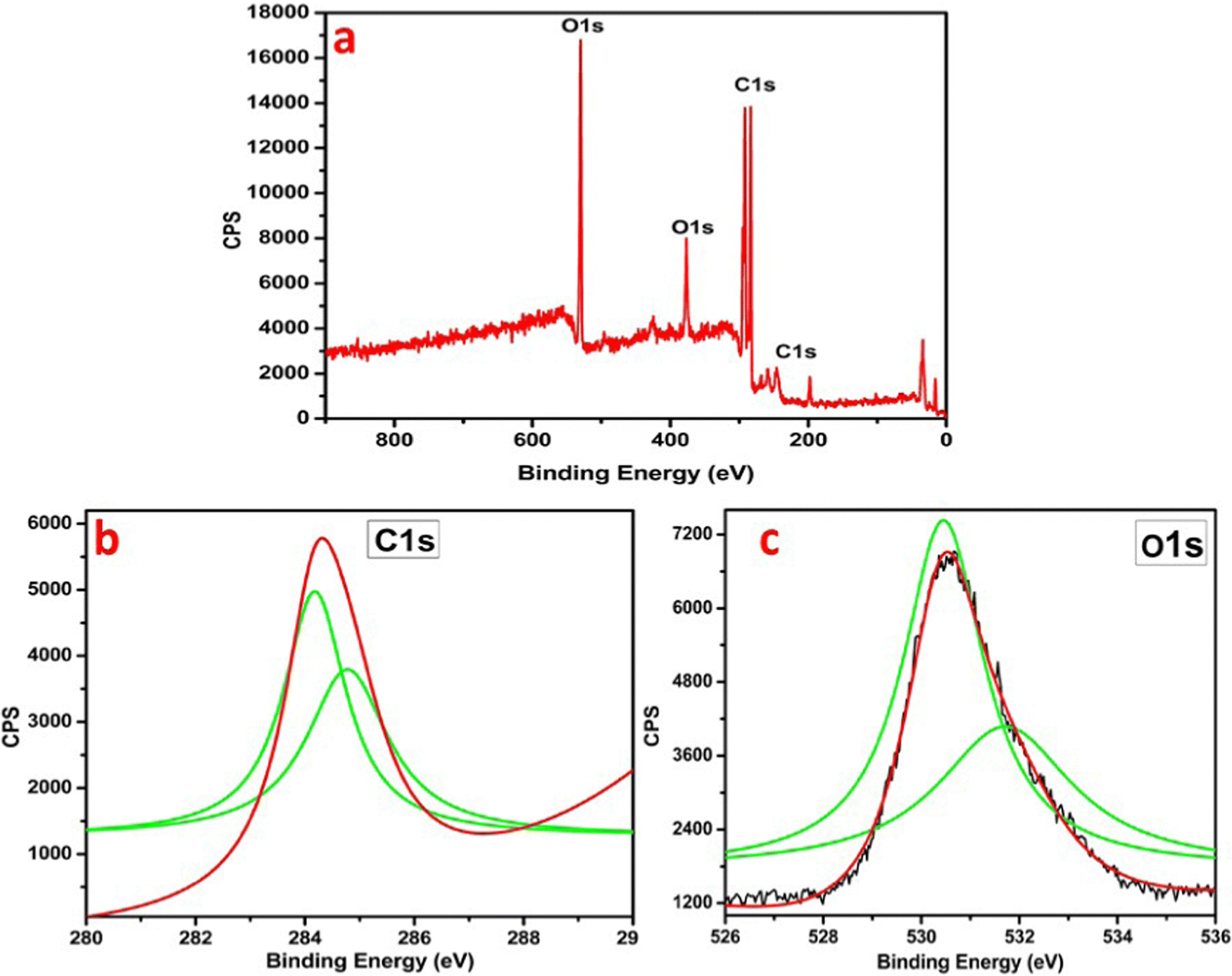Fig. 7 (a) XPS spectrum of CHG; (b) C 1s spectrum of CHG; (c) O 1s spectrum of CHG.

The XPS analysis explained the CHG sample in Fig. 7. The points of the distinctive chemical interactions between carbon, hydrogen, and oxygen are supportive for specific binding energies shown in Fig. 7. XPS analysis of CHG showed peaks at 280 eV, 282 eV, and 528 eV, 530 eV due to the carbon 1s, and oxygen 1s levels, respectively. The C 1s spectrum showed deconvoluted peaks of 1s in the Gaussian plot centered at 280 eV, 284 eV, and 286 eV for CHG (Fig. 7b). Carbon at the K-edge around 286 eV depicts a transition from its 1s state to the p* states, i.e. 1s-p* and a peak at 286 eV links to changeovers in its 1s state to the s* i.e., 1s-s* in graphene. The binding energy of the C 1s spectral component of 284.8 eV confirms the C–C and C–H bonds in the sample. Also, the K spectrum of oxygen in Fig. 7c showed peak points at 528 eV and 530 eV mainly corresponding to the p* state resonance due to the higher-order vibrations of oxygen atoms, which also can be assigned to a few advanced s* state resonances basically due to the 1,2-epoxy associations (–C=O) in the graphene films, which accurately explains the presence of a graphene skeleton.²¹ Thus, XPS analysis confirms the presence of carbon and oxygen with different functionalities in the material and confirms the synthesis of reduced graphene nanosheets.

5. Electrochemical performance testing

The two-electrode system was used to evaluate the cyclic voltammetry (CV) based analysis for the fabricated SC, and 1 M H₂SO₄ was used as the aqueous electrolyte for Cell 1. Furthermore, Cell 2 was evaluated using the polymer-gel electrolyte. CV plots of both cells were plotted at different scan rates, such as at 1 mV s⁻¹, 5 mV s⁻¹, 10 mV s⁻¹, 50 mV s⁻¹, 100 mV s⁻¹, and 200 mV s⁻¹ over a wide potential of 2 volts. For Cell 1, the plot between current (in A) and voltage (in V) discloses an EDLC behavior of the curve (Fig. 8a and b). In brief, the plot represents the formation of a double layer at the border of electrode particles and electrolyte ions, also accountable for the movement of the absolute ions. Furthermore, eqn 4 was used to compute the specific capacitance.¹⁰ Cell 1 electrodes exhibited a Cs of 650.00 F g⁻¹, and Cell 2 electrodes depicted a Cs value of 500.00 F g⁻¹ at the scan rate of 1 mV s⁻¹ (Table 3). The estimations of the Cs were studied over diverse scan rates, suggesting decent stability of the SC electrodes with growing scan rates (Table 3).

Fig. 8 (a) CV plots of cell 1, and (b) CV plots of cell 2.

Table 3 Specific capacitance (Cs) calculated using CV plots for Cell 1 and Cell 2

Scan rates (in mV s^−1)	1	5	10	50	100	200
Cs of Cell 1 (in F g^−1)	650.00	400.00	292.00	126.00	91.00	61.20
Cs of Cell 2 (in F g^−1)	500.00	290.00	230.00	140.00	90.00	60.00

---

Here, Cs is termed as the specific capacitance in F g⁻¹, is the area under the curve, m is the mass in milligrams, K is termed as the scan rate in mV s⁻¹, and ΔV is the potential in Volts.

The CV data of Cell 2 were evaluated between the same parameters and showed a similar pattern of double-layer formation between the electrode and electrolyte ions, but the surface area evaluation showed a relatively lower value of the absolute area for Cell 2 in contrast to Cell 1.

This can be attributed to the presence of protons with high ionic transportation with smaller size in the case of sulfuric acid for cell 1, and relatively lower transportation value with the larger size for polymer gel electrolyte ions as it has combined transportation of ions due to the formation of the complex polymer matrix. Although the matrix formation reduced the specific capacitance value for Cell 2, however, stability wise it can enhance the stability of the device. Furthermore, eqn (4) was used to compute the specific capacitance of both devices (Table 3). However, the stability assessment for both devices utilizing a higher scan rate of 10 mV s⁻¹ for 100 cycles showed a negligible capacitance drop and complete retention of the device performance, irrespective of the electrolyte used. However, Cell 2 at a very high scan rate of 200 mV s⁻¹ shows slight disruption in the voltammogram possibly due to overload at a high current; however, no such behavior was reported for Cell 1. Therefore, the capacitance performance of Cell 1 and Cell 2 concerning different scan rates with a potential window of 2 V are tabulated in Table 3.

Cell 1 showed a higher capacitance value due to the aqueous electrolyte and highly conductive graphene network, which showed a relatively continual decrease with increased scan rates. For instance, at 1 mV s⁻¹ a specific capacitance of 650.00 F g⁻¹ was reported, which retained 62% of the initial capacitance at 5 mV s⁻¹, 58% at 10 mV s⁻¹, 19% at 50 mV s⁻¹, 15% at 100 mV s⁻¹, and 10% at 200 mV s⁻¹. However, Cell 2 showed relatively stable performance with increasing scan rate compared to Cell 1. For instance, at 1 mV s⁻¹, a specific capacitance of 500.00 F g⁻¹ was reported, which retained 58% of the initial capacitance at 5 mV s⁻¹, 46% moving to 10 mV s⁻¹, 28% at 50 mV s⁻¹, 18% at 100 mV s⁻¹, and 12% at 200 mV s⁻¹. This depicts relatively similar performance for both devices, where Cell 1 has more capacitance and stability at lower scan rates; however, Cell 2 shows better stability at higher scan rates, which can be attributed to the presence of a polymer-gel electrolyte. Furthermore, the charging-discharging behavior of Cell 1 and 2 was estimated at different current densities of 1 A g⁻¹, 2 A g⁻¹, and 3 A g⁻¹, over the potential range of 0–1 V (Fig. 9a and b). The nearly triangular shape denotes the capacitative behavior of cell 1, while the slightly distorted triangular shape of the GCD curve represents cell 2. After very careful evaluation of the GCD plots of cell 1 and cell 2, it can be predicted that the stability of cell 2 was more in comparison to cell 1, as the discharge curve in cell 2 is more reflective with increasing current density than in the case of cell 1. Moreover, the charge-discharge plots were assessed to determine the specific capacitance (Cs) of cell 1 and cell 2 using eqn 5, and the corresponding data is tabulated in Table 4.^10,25

Fig. 9 (a) GCD plot of cell 1, and (b) GCD plot of cell 2.

Table 4 The assessed Cs from the GCD curves for Cell 1 and Cell 2

Current density (in A g^−1)	1	2	3
Cs (in F g^−1) of Cell 1	360.00	188.00	102.00
Cs (in F g^−1) of Cell 2	260.00	168.00	91.00

---

Cs denotes capacitance, i is the current density, m is the mass, and Δt/ΔV denotes the direct slope of the liberation curve.^23–25

Cell 1 displayed very high specific capacitance values at lower current density viz. 360 F g⁻¹ at 1 A g⁻¹, which decreases with an increase in current density from 2 A g⁻¹ to 3 A g⁻¹; the capacitance became 188 F g⁻¹ and 102 F g⁻¹, respectively. In addition, cell 1 showed capacitance retention of 52% moving from 1 A g⁻¹ to 2 A g⁻¹ and 30% at 3 A g⁻¹.

On the other hand, Cell 2 displayed a specific capacitance of 260 F g⁻¹ at 1 A g⁻¹, which decreases with an increase in current density from 2 A g⁻¹ to 3 A g⁻¹; the capacitance became 168 F g⁻¹ and 91 F g⁻¹, respectively. Cell 2 showed capacitance retention of 65% moving from 1 A g⁻¹ to 2 A g⁻¹ and 35% at 3 A g⁻¹. This agrees with CV data and depicts the higher stability of Cell 2 compared to Cell 1 at higher current densities; however, the capacitance values were comparatively higher for Cell 1. After CV and GCD evaluation, it is clear that Cell 1 has higher capacitance properties and lower stability at a higher potential. The current scan and Cell 2 show the opposite behavior.

Further, the variation in device performance was compared concerning scan rate and current densities, which depicted almost similar behavior for both devices. However, the pattern of capacitance drop was comparatively more profound for Cell 1. A sharp decrease is visible in Fig. 10a and b for Cell 1, which depicted a relatively quick drop in capacitance due to an aqueous electrolyte and low holding time. However, Cell 2 showed a stable departure from the initial capacitance values as visible in Fig. 10a and b, which is attributed to the stable charge-holding capability of the polymer-gel electrolyte. High capacitance values indicate high ionic movement in Cell 1, although relatively similar values with better capacitance retention at higher rates for Cell 2 suggest the good electrochemical performance of the polymer-gel electrolyte.

Fig. 10 Variation of Cs for Cell 1 and Cell 2 concerning; (a) scan rate, (b) current density.

Moreover, electrochemical impedance spectroscopy (EIS) was used to evaluate the Nyquist plots, ESR, and phase angle vs frequency response for cells 1 and 2 (Fig. 11). The graph between the impedance's imaginary part and the real part is called the Nyquist plot. The Nyquist plot (Fig. 11a) with a slope of 45 degrees at a higher frequency displays the diffusion process and is related to the penetration of ions at the pores. This is the cause behind establishing the two layers at the border of the electrode material and electrolytes. The vertical increase in the Nyquist plot at the lower frequency terminal embodies the decent capacitance behavior of cell 1. Before stability assessments, the Nyquist plot displayed very high capacitance behavior with a low value of the imaginary part of the impedance on the y-axis, which increased after stability assessments depicting depletion in capacitance for the device after stability analysis.

Fig. 11 (a) Nyquist plot of cell 1, (b) Nyquist plot of cell 2, (c) phase angle vs. frequency plot for cell 1, and (d) phase angle vs. frequency plot for cell 2.

Moreover, a lower ESR i.e. 4.75 Ω cm⁻² for cell 1, shows the good passage of ions^20–22 and agrees with capacitance analysis. Fig. 11b shows the phase angle vs. magnitude of the frequency response for Cell 1, suggesting capacitance behavior and specifying a lower resistance value for the charge transfer. Fig. 11c depicts the Nyquist plots for Cell 2 before and after stability, displaying more diffusive behavior at a higher frequency attributed to lesser ion penetration at the electrode and electrolyte interface. The lower frequency region shows the capacitance behavior of cell 2, which is better before stability assessments and declines afterward.

Nyquist plot with a higher value of the imaginary part of the impedance on the y-axis, which further increased after stability assessments depicting comparatively lower capacitance behavior in Cell 2 compared to Cell 1. Also, this is supported by an ESR value of 9.10 Ω cm⁻² and validates the existence of relatively lower capacitance for cell 2. The higher the ESR, the lower the capacitance will be as the relationship between impedance and capacitance is given by eqn (8).

Here, C is called the capacitance, f is called the frequency, and Z′′ depicts the highest impedance value on the y-axis. Fig. 11d shows the phase angle vs magnitude of the frequency response for Cell 2, suggesting a similar capacitance behavior for Cell 2 in agreement with capacitance analysis. Moreover, energy density (E_D) and power density (P_D) are powerful tools to assess the overall electrochemical performance of the SCs. Hence, we evaluated the E_D and P_D of Cells 1 and 2 using the following equations.

Here, C is called the Cs and V depicts the potential gap.

Cell 1 showed a good E_D of 50.00 W h kg⁻¹ and a P_D of 1000.00 W kg⁻¹ at 1 A g⁻¹. Similarly, cell 2 showed an E_D of 36.11 W h kg⁻¹ and a P_D of 996.92 W kg⁻¹ at 1 A g⁻¹. The evaluation showed better performance of cell 1 at a lower current density and higher performance of cell 2 at a higher current density. The values of E_D and P_D were calculated at different current densities viz. 1 A g⁻¹, 2 A g⁻¹, and 3 A g⁻¹, and are tabulated in Table 5.

Table 5 E _D and P_D for Cell 1 and Cell 2

Current density	1 A g^−1	2 A g^−1	3 A g^−1
Energy density (W h kg^−1) for Cell 1	50.00	26.11	14.16
Power density (W kg^−1) for Cell 1	1000.00	1950.92	2964.70
Energy density (W h kg^−1) for Cell 2	36.11	23.33	12.5
Power density (W kg^−1) for Cell 2	996.92	1997.14	3000

---

Based on the values of E_D and P_D a Ragone plot is displayed in Fig. 12, displaying the comparative analysis of the electrochemical performance for both devices. Cell 1 displays higher energy density in comparison to Cell 2; however the decrement in energy density for cell 2 is continual for each current density. On the other hand, for Cell 1 the decrease in energy density and increase in power density with increasing current density becomes slightly less stable justifying the performance evaluation from other parameters as well. The sudden change in energy density for Cell 1 moving from 1 A g⁻¹ to 2 A g⁻¹ depicts a quick change in stability and energy performance of the device at a higher current window showing the effects of higher current on the aqueous electrolyte. However, the continual decrement with no sudden depletion in device performance is visible in the case of Cell 2 displaying a stable performance at almost all current densities. Depicting a direct correlation with polymer gel electrolytes enhances the discharging of the device by confining the ions in the polymer matrix.^1–17 Cell 1 displays an energy density of 14.16 W h kg⁻¹ at 3 A g⁻¹, while for Cell 3 it is 12.50 W h kg⁻¹, agreeing with both statements viz. continual performance of Cell 2 at all current densities and fast drop in performance of Cell 1 at higher current densities.

Fig. 12 Ragone plot for Cell 1 and Cell 2.

After the evaluation of the energy and power density, the Coulombic efficiency was analyzed for Cell 1 and Cell 2 (Fig. 13). Cell 1 displayed a coulombic efficiency of 47.82%, 67.56%, and 45.45% at 1 A g⁻¹, 2 A g⁻¹, and 3 A g⁻¹ current densities, respectively. On the other hand, Cell 2 depicted a coulombic efficiency of 70.27%, 46.87%, and 35.71% at 1 A g⁻¹, 2 A g⁻¹, and 3 A g⁻¹ current densities, respectively. The evaluation showed a stable performance for devices at lower current densities viz. 1 A g⁻¹ and 2 A g⁻¹, and low stability at a higher current density of 3 A g⁻¹. Cell 1 showed less stability compared to Cell 2, which indicates the better stability performance of polymer gel electrolytes compared to aqueous electrolytes for SC applications.

Fig. 13 Coulombic efficiency of Cell 1 and Cell 2.

Finally, the cell stability of each cell was evaluated, in which cell 1 showed 88% performance retention for the 4400 cycles at the current density of 1 A g⁻¹; however, cell 2 showed 99% performance retention for the 4400 cycles (Fig. 14). The stability curve showed excellent cycling stability of Cell 2 in contrast to Cell 1. This suggests better stability and performance of cell 2 in contrast to cell 1. Furthermore, a comparative study was made between recently developed graphene-based materials and the current study as depicted in Table 6. These evaluations depicted that the developed material has excellent electrochemical behavior in both electrolytes and can act as a paradigm for advancing better-performing energy storage materials.

Fig. 14 Stability assessment, (a) Cell 1, and (b) Cell 2.

Table 6 Relative examination of the present study with parallel research on SCs

Materials	Electrolytes	Scan rate/current density	Specific capacitance	Stability	Ref.
Graphene powder	1 M H2SO4	10 mV s^−1	17.2 F g^−1	87.2%	23
N/S doped-graphene	PVA-H2SO4 gel electrolyte	0.05 mAcm^−2	40.4 mF cm^−2	87.6%	24
Graphene laser-induced	PVA-H2SO4	0.05 mAcm^−2	19.8 mF cm^−2	NA	25
Reduced GO	1 M H2SO4	1 A g^−1	130 F g^−1	84%	26
Graphene sheets	6 M KOH	1 A g^−1	282 F g^−1	70%	27
Waste plastic-derived graphene	1 M H3PO4	5 mV s^−1	139.7 F g^−1	82%	4
Agriculture waste-derived graphene	PVA–H3PO4	5 mV s^−1	18.2 F g^−1	85%	11
Tire waste-derived graphene	1 M H2SO4	5 mV s^−1	316 F g^−1	86%	28
Coconut husk-derived graphene	1 M H2SO4	1 mV s^−1	650 F g^−1	88%	This work
Coconut husk-derived graphene	PVA-KI-H2SO4	1 mV s^−1	500 F g^−1	99%	This work

---

6. Conclusion

This work reports a new and economical approach to the bulk-scale synthesis of reduced graphene oxide. Raman, XRD, XPS, SEM/EDX analysis, and TEM analysis confirmed the synthesis of reduced graphene oxide. The developed materials showed good electrochemical properties in 1 M H₂SO₄ and PVA-KI-H₂SO₄ polymer gel electrolytes. The CV analysis of cell 1 showed the highest specific capacitance of 650 F g⁻¹ at 1 mV s⁻¹. The GCD analysis showed 88% performance retention for the 4400 cycles at 1 A g⁻¹, which depicted the good performance of cell 1. However, cell 2 showed a specific capacitance of 500 F g⁻¹ at 1 mV s⁻¹ with 99% stability up to 4400 cycles. Cell 1 displayed an E_D of 50.00 W h kg⁻¹ and a P_D of 1000.00 W kg⁻¹ at 1 A g⁻¹, while Cell 2 showed an E_D of 36.11 W h kg⁻¹ and a P_D of 996.92 W kg⁻¹ at 1 A g⁻¹. The evaluation showed better performance of cell 1 at a lower current density and stable performance of cell 2 at all current densities. The device's performance can be boosted with the help of variations in electrolytes, mixing of activated carbon, and varying device fabrication conditions. Also, the higher stability of the developed material in the polymer-gel system opens up new insights for advancing reduced graphene and polymer gel-based electrolyte-based devices for high-performance supercapacitors. This material will be beneficial for fabricating better-performing SCs for different energy applications.

Conflicts of interest

The authors state no opposing interests.

Acknowledgements

The authors would like to thank the National Mission of Himalayan Studies (NMHS), Kosi Katarmal, Almora, India (Ref. No. GBPNI/NMHS-2019-20/MG), Project Sutram DST (Ref No.: DST/TM/WTI/WIC/2K17/82(G)), DST INSPIRE Division (Ref. No.- IF180347), New Delhi, India, and DST-FIST Delhi, India for their monetary funding, and the Kempe Foundation is gratefully acknowledged for the financial support (grant number: SMK-1945). Chetna Tewari acknowledges the Korean Institute of Science and Technology, South Korea, for funding.

References

1. M. Ripa, G. Fiorentino, H. Giani, A. Clausen and S. Ulgiati, Refuse recovered biomass fuel from municipal solid waste. A life cycle assessment, Appl. Energy, 2017, 186, 211–225.
2. H. Zhou, A. Meng, Y. Long, Q. Li and Y. Zhang, An overview of characteristics of municipal solid waste fuel in China: physical, chemical composition and heating value, Renewable Sustainable Energy Rev., 2014, 36, 107–122.
3. G. Tatrari, M. Karakoti, M. Pathak, A. Dandapat, T. Rath and N. Gopal Sahoo, Quantum dots based materials for new generation supercapacitors application: a recent overview, Quantum Dots and Their Applications, 2021, vol. 96, p. 215.
4. N. Sahoo, G. Tatrari, C. Tewari, M. Karakoti, B. S. Bohra and A. Danadapat, Vanadium pentaoxide-doped waste plastic-derived graphene nanocomposite for supercapacitors: a comparative electrochemical study of low and high metal oxide doping, RSC Adv., 2022, 12(9), 5118–5134.
5. M. Karakoti, S. Pandey, G. Tatrari, P. S. Dhapola, R. Jangra, S. Dhali, M. Pathak, S. Mahendia and N. G. Sahoo, A waste to energy approach for the effective conversion of solid waste plastics into graphene nanosheets using different catalysts for high performance supercapacitors: a comparative study, Mater. Adv., 2022, 3(4), 2146–2157.
6. G. Tatrari, M. Karakoti, C. Tewari, S. Pandey, B. S. Bohra, A. Dandapat and N. G. Sahoo, Solid waste-derived carbon nanomaterials for supercapacitor applications: a recent overview, Mater. Adv., 2021, 2(5), 1454–1484.
7. C. Tewari, G. Tatrari, S. Kumar, S. Pandey, A. Rana, M. Pal and N. G. Sahoo, Green and cost-effective synthesis of 2D and 3D Graphene-based nanomaterials from Drepanostachyum falcatum for Bio-imaging and Water purification applications, Chem. Eng. J. Adv., 2022, 100265.
8. B. Andonovic, A. Ademi, A. Grozdanov, P. Paunović and A. T. Dimitrov, Enhanced model for determining the number of graphene layers and their distribution from X-ray diffraction data, Beilstein J. Nanotechnol., 2015, 6(1), 2113–2122; M. Parikka, Biomass Bioenergy, 2004, 27, 613–620.
9. J. Ribeiro-Soares, M. E. Oliveros, C. Garin, M. V. David, L. G. P. Martins, C. A. Almeida, E. H. Martins-Ferreira, K. Takai, T. Enoki, R. Magalhães-Paniago and A. Malachias, Structural analysis of polycrystalline graphene systems by Raman spectroscopy, Carbon, 2015, 95, 646–652.
10. S. M. Clark, K. J. Jeon, J. Y. Chen and C. S. Yoo, Few-layer graphene under high pressure: Raman and X-ray diffraction studies, Solid State Commun., 2013, 154, 15–18.
11. G. Tatrari, C. Tewari, M. Karakoti, M. Pathak, R. Jangra, B. Santhibhushan, S. Mahendia and N. G. Sahoo, Mass production of metal-doped graphene from the agriculture waste of Quercus ilex leaves for supercapacitors: inclusive DFT study, RSC Adv., 2021, 11(18), 10891–10901.
12. S. Gillet, M. Aguedo, L. Petitjean, A. R. C. Morais, A. M. da Costa Lopes, R. M. Łukasik and P. T. Anastas, Lignin transformations for high value applications: towards targeted modifications using green chemistry, Green Chem., 2017, 19(18), 4200–4233.
13. G. A. Ferrero, A. B. Fuertes and M. Sevilla, N-doped porous carbon capsules with tunable porosity for high-performance supercapacitors, J. Mater. Chem. A, 2015, 3(6), 2914–2923.
14. Z. Spitalsky, D. Tasis, K. Papagelis and C. Galiotis, Carbon nanotube–polymer composites: chemistry, processing, mechanical and electrical properties, Prog. Polym. Sci., 2010, 35(3), 357–401.
15. J. Liang, H. Zhao, L. Yue, G. Fan, T. Li, S. Lu, G. Chen, S. Gao, A. M. Asiri and X. Sun, Recent advances in electrospun nanofibers for supercapacitors, J. Mater. Chem. A, 2020, 8(33), 16747–16789.
16. Y. Yang, Y. X. Liu, Y. Li, B. W. Deng, B. Yin and M. B. Yang, Design of compressible and elastic N-doped porous carbon nanofiber aerogels as binder-free supercapacitor electrodes, J. Mater. Chem. A, 2020, 8(33), 17257–17265.
17. S. You, X. Xi, X. Zhang, H. Wang, P. Gao, X. Ma, S. Bi, J. Zhang, H. Zhou and Z. Wei, Long-term stable and highly efficient perovskite solar cells with a formamidinium chloride (FACl) additive, J. Mater. Chem. A, 2020, 8(34), 17756–17764.
18. G. Tatrari, C. Tewari, M. Pathak, D. Bhatt, M. Karakoti, S. Pandey, D. S. Uniyal, F. U. Shah and N. G. Sahoo, 3D-graphene hydrogel and tungsten trioxide-MnO2 composite for ultra-high-capacity asymmetric supercapacitors: A comparative study, J. Energy Storage, 2023, 68(15), 107830.
19. R. Vicentini, J. P. Aguiar, R. Beraldo, R. Venâncio, F. Rufino, L. M. Da Silva and H. Zanin, Ragone Plots for Electrochemical Double-Layer Capacitors, Batteries Supercaps, 2021, 4(8), 1291–1303.
20. K. Liu, M. Wu, H. Jiang, Y. Lin and T. Zhao, An ultrathin, strong, flexible composite solid electrolyte for high-voltage lithium metal batteries, J. Mater. Chem. A, 2020, 8(36), 18802–18809.
21. G. Li, Y. Wang, H. Guo, Z. Liu, P. Chen, X. Zheng, J. Sun, H. Chen, J. Zheng and X. Li, Direct plasma phosphorization of Cu foam for Li ion batteries, J. Mater. Chem. A, 2020, 8(33), 16920–16925.
22. L. Guardia, L. Suárez, N. Querejeta, V. Vretenár, P. Kotrusz, V. Skákalová and T. A. Centeno, Biomass waste-carbon/reduced graphene oxide composite electrodes for enhanced supercapacitors, Electrochim. Acta, 2019, 298, 910–917.
23. N. Samartzis, M. Athanasiou, V. Dracopoulos, S. N. Yannopoulos and T. Ioannides, Laser-assisted transformation of a phenol-based resin to high quality graphene-like powder for supercapacitor applications, Chem. Eng. J., 2022, 430, 133179.
24. M. Khandelwal, C. Van Tran, J. Lee and J. B. In, Nitrogen and boron co-doped densified laser-induced graphene for supercapacitor applications, Chem. Eng. J., 2022, 428, 131119.
25. K. Y. Kim, H. Choi, C. Van Tran and J. B. In, Simultaneous densification and nitrogen doping of laser-induced graphene by duplicated pyrolysis for supercapacitor applications, J. Power Sources, 2019, 441, 227199.
26. T. X. Tran, H. Choi, C. H. Che, J. H. Sul, I. G. Kim, S. M. Lee, J. H. Kim and J. B. In, Laser-induced reduction of graphene oxide by intensity-modulated line beam for supercapacitor applications, ACS Appl. Mater. Interfaces, 2018, 10(46), 39777–39784.
27. K. Nanaji, V. Upadhyayula, T. N. Rao and S. Anandan, Robust, environmentally benign synthesis of nanoporous graphene sheets from biowaste for ultrafast supercapacitor application, ACS Sustainable Chem. Eng., 2018, 7(2), 2516–2529.
28. G. Tatrari, C. Tewari, M. Pathak, B. S. Bohra, M. Karakoti, S. Pandey, B. Santhibhushan, A. Srivastava, S. Rana and N. G. Sahoo, Bulk Production of Zinc Doped Reduced Graphene Oxide from Tire Waste for Supercapacitor application: Computation and Experimental Analysis, J. Energy Storage, 2022, 53, 105098.

---

Footnotes

† Electronic supplementary information (ESI) available. See DOI: https://doi.org/10.1039/d3ma00126a

‡ Both authors contributed equally to this manuscript.

---