High-precision, low-complexity, high-resolution microscopy-based cell sorting

Abstract

Continuous flow cell sorting based on image analysis is a powerful concept that exploits spatially-resolved features in cells, such as subcellular protein localisation or cell and organelle morphology, to isolate highly specialised cell types that were previously inaccessible to biomedical research, biotechnology, and medicine. Recently, sorting protocols have been proposed that achieve impressive throughput by combining ultra-high flow rates with sophisticated imaging and data processing protocols. However, moderate image quality and high complex experimental setups still prevent the full potential of image-activated cell sorting from being a general-purpose tool. Here, we present a new low-complexity microfluidic approach based on high numerical aperture wide-field microscopy and precise dielectrophoretic cell handling. It provides high-quality images with unprecedented resolution in image-activated cell sorting (i.e., 216 nm). In addition, it also allows long image processing times of several hundred milliseconds for thorough image analysis, while ensuring reliable and low-loss cell processing. Using our approach, we sorted live T cells based on subcellular localisation of fluorescence signals and demonstrated that purities above 80% are possible while targeting maximum yields and sample volume throughputs in the range of μl min⁻¹. We were able to recover 85% of the target cells analysed. Finally, we ensure and quantify the full vitality of the sorted cells cultivating the cells for a period of time and through colorimetric viability tests.

---

1. Introduction

The identification and isolation of single cells or subsets of cells with unique physiological properties from heterogeneous cell populations has become a necessity in biotechnology and biomedical research.^1–3 Nowadays it is clear that the physiological properties of a cell are strongly linked to its morphology.^4–11 Conventional sorting methods that employ low-resolution sorting parameters, like one-dimensional fluorescence signals or scattered light integrated from the whole cell, ignore the spatial information of the signal distribution over the cell.^1,12–15 Therefore, they miss out on substantial features important for the development of new therapeutic approaches, single cell research,^5,16–19 bioproduction²⁰ and drug development.²¹

To overcome this limitation, various high-impact works have been published in the recent years, combining sorting with bright field and fluorescence 2D-imaging data and thus being able to make spatial cues in cells (e.g., subcellular localisation of fluorescently-labelled markers, protein co-localisation etc.) accessible for cell classification and sorting.^12,22–28

In image-activated flow sorting, the correct alignment of the cells in the central focal plane is essential to achieve high image quality and high control over cell movement. For this purpose, the width of the sample stream is usually confined to a few μm, either by 3D sheath flows^22,28 or small constriction channels.²⁴ Nevertheless, to achieve a high sample volume throughput (i.e., at least in the range of μl min⁻¹), high flow velocities of up to 1 m s⁻¹ must be applied.

At such high flow velocities, imaging of faint fluorescence signals, data processing and sorting have to take place within microseconds, which is technically enormously demanding. As a result, the proposed systems are complex, require elaborate imaging-, flow control- and data management mechanisms and are still limited in the achievable image quality and depth of analysis.^22,23,26,28

In cell biology, however, spatial information with nm precision can be crucial. This is the case, for example, when analysing subcellular structures such as mitochondria or cytoskeleton or the close interaction of proteins and their localisation within the cell.^29,30 In this respect, fluorescence microscopy via direct imaging offers a good compromise between high image quality, high resolution and low system complexity. However, to use this widely used technique for blur-free imaging under flow, it is necessary to work with flow velocities several orders of magnitude lower than in the studies mentioned above, as the acquisition of fluorescence images with commercially available cameras offers only limited frame rates and requires relatively long integration times (i.e., in the sub-ms range).

In this paper, we present a low-complexity microfluidic approach that enables flow-through image-based cell analysis and precise sorting based on standard high numerical aperture wide field microscopy, achieving a level of image quality comparable to steady state conditions. To be able to work at the low flow velocities required by the image acquisition and still achieve both a reasonable sample throughput in the μl min⁻¹ range and a precise control of the cell position in the channel, we focus the cells in the microchannel by the well-established concept of dielectrophoresis^31–36 instead of confining the sample flow.

Besides focusing, we also employ dielectrophoretic forces to sort the cells. Taking advantage of the high precision of microelectrode fabrication, we are able to reduce the effective length of the sorting window (i.e., the minimum distance between two consecutive cells to be sorted independently) almost down to the size of a single cell. This allows us to achieve high purity and yield even for very dense cell samples, the latter being a prerequisite for processing an acceptable number of cells in a reasonable amount of time even at low flow velocity.

Thanks to the simple and robust concept of our sorting protocol, no external instruments other than microfluidic pumps and a multichannel signal generator are required to control the cell flow in our system. Furthermore, the frame rates and associated amount of data to be processed are comparably small, so that a standard Windows PC is sufficient to operate the whole system.

We demonstrated the ability of our low-complexity image-activated cell sorter to sort out cells from heterogeneous cell samples based on image processing (i.e., extraction of pure colour information or the spatial distribution of subcellular fluorescence signals). By maximising sorting yields at the expense of cell throughput, we achieved target cell purities between 80% and 95% at yields around 85%.

Besides the performances of the sorting, maintaining cell health and viability is a fundamental requirement for any cell sorter. However, the high shear stress to which the cells are subjected when moving through very small channels at high speed, as well as cell-stressing sheath buffer compositions are often a limiting factor to achieve desirable vitality levels. We do not use sheath buffers, so the cells remain in their preferred medium throughout the complete sorting process as dielectrophoretic cell handling in physiological medium is still possible when using negative dielectrophoresis.^37,38 To demonstrate the high biocompatibility of our gentle and low-shear rate process, we show and quantify the vitality of the sorted cells through both colorimetric viability assays and continuation of the processed cells in cell culture.

2. Results

2.1 Microfluidic system and cell processing

The system is depicted in Fig. 1a. It consists of a 650 μm wide microchannel made of two glass plates and a 35 μm thick polymer spacer, as described earlier.^37,38 The channel features two inlets for sample cells and buffer, and two outlets for target and waste cells and is placed on a standard inverted fluorescence microscope equipped with a high numerical aperture objective and a state-of-the art CMOS camera.

Fig. 1 Schematic overview of the microfluidic system and the dielectrophoretic sorting principle (not to scale). a, Top view of the microchannel. Top and bottom glass slides of the microchannel are equipped with congruent microelectrodes (black lines) which cells can initially pass freely unless an electric field is applied between them (1 MHz, 3 to 4.5 V, depending on the electrode pair). In this case, the electrode segment acts as a barrier for the cells (flowing at 580 μm s⁻¹ or 40 μl h⁻¹), deflecting them from their path through the channel. A cell sample containing target and non-target cells (depicted in red and green, respectively) is introduced into the microfluidic channel through the sample inlet. Buffer from a second inlet ensures that the opposing half of the microchannel and target cell outlet are not accidently contaminated with cell debris from the sample inlet. Electrode pairs E1 and E2 focus all cells into a pearl chain configuration. A CMOS camera continuously captures images of the region of interest (ROI), which are analysed by a standard PC for the presence and velocity of target cells. On this basis, an activation pattern of the sorting electrode array E3 is generated and transmitted to the electrodes via a signal generator. After the sorting step (details in b), target and non-target cells are further separated by electrode pair E4, forwarded to the respective outlets and recovered from the system. b, Time series of enlarged schematic of the ROI and sorting electrode array E3 (red frame) for channel top view. t₁: Target and non-target cells arrive one after the other at the ROI. The system automatically detects target cells and tracks their position. t₂: The position of the detected target cell is tracked continuously across multiple frames and its velocity is calculated. Non-target cells pass the eight individual electrodes of the sorting electrode array which remain inactive. t₃: Based on the calculated target cell velocity, the targeted activation of individual sorting electrodes ensures that each target cell is deflected. t₄: The subsequent electrodes are activated according to the flow velocity of the target cell to achieve complete separation of the cells. c, Depiction of different force effects on cells flowing in the microchannel with active electrodes (channel side view). In addition to the hydrodynamic force F_H exerted by the fluid flow and driving the cells through the channel, the gravitational force F_G and the buoyant force F_B act with constant strength. The dielectrophoretic force F_DEP acts towards the minimum of the gradient of the electric field generated by the electrodes, which is located in the vertical centre of the channel in front of the electrodes. If the field strength is sufficient, F_H and horizontal component of F_DEP are in equilibrium, preventing cells from passing through the electrodes. At the same time, an equilibrium is established between F_B, F_G and the vertical component of F_DEP, whereby the cells arrange in a common vertical plane. For information on electric field distribution between active electrodes, please see ref. 37.

Pressure-driven flow is used to hydrodynamically drive the cells through the channel while several platinum electrodes extending in different geometries along the channel deflect the cells across flow lines by dielectrophoretic forces. The electrodes are arranged in pairs on the top and bottom inner faces of the microchannel and were supplied with square-wave radio frequency electric signals between 3 V and 4.5 V peak-to-peak by custom-made signal generators. Cells brought by the flow into the immediate vicinity of the electrodes are polarised and experience a force directed to the minimum of the electric field gradient (i.e., dielectrophoresis). Due to the pairwise arrangement of the electrodes at top and bottom of the channel, the resulting force vector has both a horizontal and a vertical component directed towards the central plane of the microchannel^39,40 (Fig. 1c). For details on dielectrophoresis and the function of the microfluidic chips see ref. 37, 38 and 41.

The different electrode pairs along the channel (see also ESI,† Fig. S1) serve different purposes. At the beginning of the channel, long transversing electrodes (E1 and E2 in Fig. 1a) focus cells into a streamline. The subsequent sorting array (E3 in Fig. 1a) consists of eight consecutive short electrodes that are operated sequentially (Fig. 1b). The length of the individual electrodes has a direct impact on the precision of sorting target cells, as it determines the effective length of the sorting window. Due to the short length of only 50 μm of the individual electrode segments, only a small cell spacing is required for efficient sorting of target cells, which enables the processing of high cell densities (see ESI†).

Finally, diverging electrodes (E4 in Fig. 1a) further separate target and non-target cells and guide them towards different channel outlets. Here, the target cells are forwarded to a rinsing flow, flushed out of the system and collected into standard cell culture equipment.

The analysis of the cells is based on a series of high-quality images that are acquired for each cell in the region of interest directly in front of the sorting array. The velocities of the cells are calculated after tracking them according to the central coordinates of the cells in several consecutive frames (Fig. 1b). In the case of a target cell, the computer switches sequentially individual sorting electrodes according to the expected position for each target cell.

2.2 Cell vertical focussing & cell velocity distribution

Cells introduced into the microchannel are initially equally distributed over the entire channel lumen (both vertically and horizontally), so they need to be confined in both spatial directions for proper imaging and sorting. A key feature of our system is the ability to not only confine the cells horizontally but also to force them into the central vertical plane of the microchannel when driven along the active electrodes (Fig. 1c). This eliminates the need for 3D sheath flow architectures to bring the cells into focal plane before image acquisition, which would dilute the sample and accelerate the cells. To demonstrate this self-focusing effect, we analysed cells flowing through the channel at 580 μm s⁻¹ while the transversing electrodes (E1 and E2 in Fig. 1a) were both active and inactive, respectively. Fig. 2b and c show exemplary images of cells for each condition (see also ESI,† Fig. S3). While in the case of active electrodes the majority of the cells were located in a common focal plane (Fig. 2c), in the case of inactive electrodes the vertical position of the cells varied considerably (Fig. 2b). Due to the parabolic velocity profile in the microchannel the variability of vertical position is also reflected by the velocity distribution of the cells. To this end, we measured the velocity of each cell and determined the frequency distribution of the cell velocity for both experiments (see Fig. 2a). The plot shows both a higher average velocity and a narrower velocity distribution when the cells were guided by the electrodes compared to cells that did not interact with the electric field of the deflection electrodes but flowed freely through the channel.

Fig. 2 Frequency distribution of cell velocity and vertical alignment of dielectrophoretically guided cells compared to free-flowing cells. While flowing through the microchannel, cells were either dielectrophoretically guided (i.e. electrodes active) or free flowing (i.e. electrodes inactive). Images of the cells were taken and their velocity determined as they appeared in the ROI. a: Frequency distribution of velocity of dielectrophoretically guided (blue) and free-flowing cells (orange). Free-flowing cells exhibited a much broader velocity distribution than dielectrophoretically guided cells, due to the random vertical distribution of the cells in the microchannel and the associated different flow regimes of the parabolic flow profile in which they were located. In contrast, the dielectrophoretically guided cells experienced a vertical force that directed them into a common vertical plane and flow regime, equalising their velocities. b and c: Exemplary images of free-flowing (b) and dielectrophoretically guided cells (c). The different vertical positions of free-flowing cells were also reflected by the highly variable image sharpness. In contrast, the dielectrophoretically-guided cells were perfectly aligned in focus. The numbers in white represent the measured velocity of each cell in μm s⁻¹. Scale bar, 20 μm. A larger overview can be found in the ESI† in Fig. S3.

2.3 Characterisation of the sorting process

To evaluate the general sorting performance of the proposed cell sorter, we prepared a sample of 10% red and 90% green cytosol-stained cells. We conducted a series of so-called “yield sortings”, where the goal is to collect a maximum amount of target cells, irrespective of possible contamination with closely neighbouring non-target cells. The sortings were conducted across several days with varying cell densities and a running time of at least 60 minutes. The cells were imaged at a 60× magnification. The red (target) cells were sorted and driven to the target cell outlet and collected in a 2 mL Eppendorf vessel while green (i.e., non-target) cells were forwarded to the waste outlet (see Fig. 1a). The samples of the collected target cells were transferred to a standard 96 well plate and imaged using an automated live-cell imaging system (Olympus IXplore Live with ScanR). Based on the images, we evaluated the target cell concentration. With our sorting system we achieved target cell purities between 95% at a throughput of 2000 cells per h and 72% at a throughput of 12 000 cells per h. Fig. 3a shows the individual data points as well as the theoretical target cell purities that can be expected from Poisson statistics. For details, see ESI.†Fig. 3b shows exemplary fluorescent images of a cell sample before and after sorting at 60× magnification at a throughput of ca. 12 000 cells per h.

Fig. 3 Evaluation of the colour-based sorting performance of the system. a, The achieved target cell purity as a function of cell throughput for sortings at 60× magnification. Experimental results are depicted in blue while the orange line indicates ideal results based on Poisson's statistics (see ESI† for theoretical description). b, Representative images of a cell sample initially containing 10% of red cytosol-stained cells and 90% of green cytosol-stained cells before (left) and after sorting red cytosol-stained cells as target cells (right) at a throughput of 12 000 cells per h. For visualisation, the colour channels of four individual images were thresholded, colour corrected, merged and stitched together with ImageJ. The figure shows representative image sections, the scale bar represents 200 μm.

To investigate the cell recovery rate and the precision of the sorting process in more detail, we repeated the sorting of red and green cytosol-stained cells as described above but at a lower magnification (i.e., 4×), enabling the observation of the whole sorting array during operation. A corresponding sorting sequence is shown in ESI† Video S1.

Counting of target cells in the recorded videos of the “yield sorting” experiments at low magnification revealed that our system correctly identified and sorted ca. 96% of the total analysed red target cells into the target outlet. We also compared the actual amount of target cells recollected from the device with the number of target cells counted in the recorded videos before sorting at 60× and at 4× magnification. On average, 85% of all analysed target cells were successfully sorted and recollected from the system with a standard deviation of only 5% over all sorting experiments (see ESI† Table S1). Both purity and recovery rate of the sorted sample kept constant along the whole experimental time, as well as in between independent repetitions. Across all experiments, the system was stable and did not require any external intervention for the entire duration of the experiment, which in some cases lasted up to 4 hours.

2.4 Morphology-based real time cell sorting

To demonstrate the full potential of an image-based cell sorting and the quality of the acquired images, we sorted cells based on spatial characteristics (details of the sorting decision are included in ESI†). For this purpose, we prepared a cell sample consisting of 10% target cells and 90% non-target cells stained with a (red fluorescent) membrane- or cytosol dye, respectively. For clear differentiation after sorting, the target and non-target cells were additionally labelled with a green fluorescent cytosol and blue fluorescent DNA dye, respectively. However, the basis for the sorting decision was exclusively the information of the red fluorescence. In this colour channel, the membrane-stained cells appear like a doughnut in the high-quality images (Fig. 4a) due to the major dye concentration at their external membrane while the cytosol-stained cells show a gradually-increasing fluorescence signal towards their centre, as expected from the 2D projection of homogeneous 3D dye distribution within the cytosol. For the classification of a cell into target or non-target cell, sixteen radially evenly distributed brightness profiles across the outer cell boundary were analysed (Fig. 4b and c). Profiles with continuously increasing brightness values in the direction towards the cell centre were defined as C-type. Those that had a maximum value in the outer region and dropped to below 90% of this value in the direction of the cell centre were defined as M-type profiles according to the high localisation of the fluorescence signal in the membrane. While cytosol-stained cells showed almost exclusively C-type profiles, membrane-stained cells did not only show M-type profiles but also C-type profiles due to some spot-like inhomogeneities of the fluorescence staining (see Fig. 4a). Based on the number of C- and M-type profiles among these sixteen profiles, the cell was classified as either membrane- or cytosol-stained (see also ESI† Video S2). To build our classification algorithm, we used a dataset of approximately 1000 images of isolated membrane- and cytosol-stained cells and determined the number of M-type profiles for each cell. We studied the sensitivity and specificity of cell classification and determined the expected purity of the sorted cell sample for different classification criteria and target cell concentrations of the initial sample (see Tables S2 and S3 in ESI†). On this basis, we decided to classify a cell with at least three M-type profiles out of sixteen as a membrane-stained cell. The sorting performances associated to this classification criteria are: sensitivity 80%, specificity 99% and 96% purity for a ratio of 10% target and 90% non-target cells. This translates to less than 5% of error in the purity of the experimental image-based sorting being related to the classification decision.

Fig. 4 Image analysis. a, Exemplary images of cytosol- (first row) and membrane-stained cells (second row) flowing in the microchannel at approximately 580 μm s⁻¹. The micrographs were taken at 60× magnification and 0.5 ms exposure time. Scale bar, 10 μm. b and c, Basics for classification of cytosol- and membrane-stained cells, respectively. For each cell, sixteen radially equally distributed brightness profiles across the outer cell border were collected and each normalised for brightness and profile length, respectively. Cytosol-stained cells usually show brightness profiles with gradually increasing values towards the cell centre, as depicted in (b). However, most of the membrane-stained cells show a large number of brightness profiles with a maximum value in the outer region and decreasing values towards the cell centre, which is associated with a higher concentration of fluorescence in the membrane (c). Profiles that fall below the threshold of 0.9 after reaching the maximum value are defined as M-type profiles (marked in orange), while profiles that do not fall below this threshold are defined as C-type profiles (marked in blue). After testing various classification criteria, those cells were classified as membrane-stained that had at least three or more M-type profiles among the sixteen profiles (see ESI†).

Once the classification parameters were defined, we conducted a series of sorts across two different days at different cell densities with a running time of approximately 30 minutes each. Cells were again imaged at 60× magnification and sorted according to their subcellular brightness distribution. The sorted cells were recollected from the system, analysed by fluorescence microscopy and target cell purity was assessed by human-based counting of cells in the images. For this morphology-based sorting we achieved target cell purities of up to 83% and enrichment factors between 4.1 and 11.9 (see Table 1).

Table 1 Experimental data of the morphology-based real time cell sorting

Throughput	Analysed cells		Target cell concentration		Enrichment
(cells per h)	Total	Target	Initial	Final	Factor
1206	1069	214	20.0%	83.0%	4.1
1491	1341	108	8.1%	61.0%	7.6
2789	1229	248	20.2%	82.2%	4.1
3960	3467	240	6.9%	82.6%	11.9
7692	6902	645	9.3%	76.5%	8.2

---

2.5 Cell vitality assessment

To rule out potentially deleterious effects of our system on cells, we assessed the viability of the processed cells by a standard colorimetric tetrazolium salt assay and cell counting. For that, a (non-stained) cell sample was processed in the system with the sorting electrodes constantly switched on. A reference cell sample was kept at room temperature for the duration of the experiment. One fraction of each sample was directly analysed for cell number, treated with the assay solution and analysed for absorbance per cell. The remaining fractions were transferred to cell culture flasks, cultured over the following one or two days, and analysed afterwards in the same way.

The results of this experiment are shown in Fig. 5. The normalised cell growth of the reference sample increased throughout the observed days. After a short lag phase, the cell number of the sorted sample followed this increase. The measured absorbance, normalised to cell number, was comparable for both samples, with a slight increase over the days.

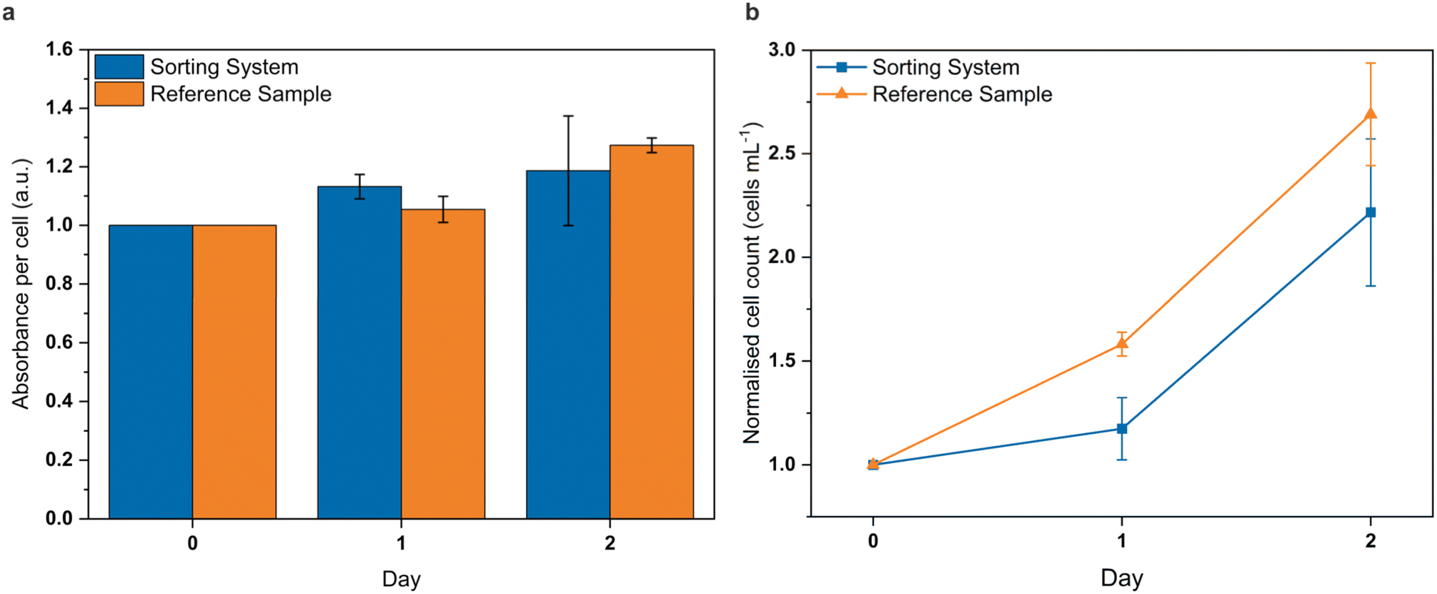Fig. 5 Vitality of processed cells. a, Photometrically-measured normalised absorbance per cell over the course of two days after treatment with a standard colorimetric tetrazolium salt assay for a cell sample that was passed through the sorting system under standard sorting conditions (square-blue) and a reference sample that was not flushed through the system but otherwise treated in the same way (triangle-orange). b, Corresponding normalised cell growth of both samples over two days.

3. Discussion

The presented technology combines technical simplicity, flexibility and robustness with high-precision cell handling and high-resolution imaging, setting it apart from existing methods (see ESI† Table S4). This is possible for several reasons: (i) all the active actuations on the cells inside the device for cell handling, focusing and sorting rely on only one physical principle: the balance between hydrodynamic and DEP forces (see Fig. 1 and 2). (ii) Thereby, we achieve an acceptable sample volume throughput in the range of μl min⁻¹ without the need for high flow velocities associated with commonly used sample stream confinement for cell focusing. (iii) This makes standard fluorescence microscopy via direct imaging applicable for the analysis of the cells, which is robust and provides high-resolution image data with little effort.

Fig. 4a shows the level of image quality achieved by the system when cells flow at 580 μm s⁻¹. The detailed morphology of the cells and the high resolution of the images (i.e., 9.3 px μm⁻¹) without blurring is comparable to the image quality achieved under stationary conditions. The acquisition of these fluorescent images requires a relatively long (500 μs) exposure time, which only leads to non-blurred images when flow velocities are low.

The importance of high-quality images to identify morphological differences between groups of cells and to use them for cell sorting applications is evident in recent works where the high capabilities of artificial intelligence using convolutional neuronal network (CNN) approaches help to classify and even sort blood cells based on label-free bright field images.^42–44 These results highlight the major importance of having high-quality images of the cells to detect unexpected morphological patterns that only an algorithm can identify after processing thousands of cells. We believe that high-quality microscopy (bright field in the combination with fluorescence) is fundamental for linking physiological properties of a cell to its morphology.

In this regard, a remarkable feature of our system is that the time available for image analysis can be adjusted according to computing time requirements. This is done by simply adjusting the relative position of the cell inspection area with respect to the sorting microelectrodes. Due to the fact that the movement of the cells in the microchannel along the electrodes is well-controlled and kept in a precise vertical plane, the cells can travel long distances (i.e., several mm) without the need for additional control of speed and trajectory, unlike other systems.^22,23 The velocity of each cell is calculated individually, making possible to create an expected trajectory for each cell.

The controlled movement in combination with the low speed of the cells (i.e., a few hundred μm s⁻¹) supports image analysis times in the order of hundreds of milliseconds. This flexibility in decision time opens up the possibility to combine our system with more advanced artificial intelligent computing.^43,45 Apart of that, the long frame acquisition and processing times reduced the amount of data and allowed us to use a colour camera, including processes of Debayering and on-line dynamic range colour adjustment for each frame. This is advantageous, since large amounts of data require a more complex data management that would exceed the capabilities of a standard PC.

The low flow velocities in our system are achieved without compromising the sample volume flow rate (i.e., lower μl min⁻¹ range), keeping the real amount of total processed sample per time acceptable. This property is described by the ratio of sample volume throughput to flow velocity (we call this factor “flow efficiency”) and is compared for different approaches to image-based cell sorting in Table S4 (see ESI†). The flow efficiency of our system is orders of magnitude larger than other approaches, as our approach does not require 3D hydrodynamic cell confinement or the use of a small channel cross-section to control the position of the cells along the microchannel.

The performance of a cell sorting process in terms of throughput, yield and purity also depends on the so-called sorting window (i.e., the minimum distance accepted by the sorter to distinguish between two different cells). Our proposed concept of handling the cells by stepwise-arranged microelectrodes allows the active sorting window to be extremely small, down to the size of the object to be sorted, by just reducing the length of the sorting electrodes. This permits working with relatively high particle densities, which leads to reasonable throughputs even at low flow rates. It is easy to see that the sorting window in our approach can be further reduced by a factor of 3–5, which would allow processing of 3–5 times more concentrated cell samples, increasing throughput by the same amount without compromising image quality or other sorting parameters. The size of the sorting window has also a direct impact on the maximum achievable ratio between yield and purity of the sort. The fact of having small sorting windows makes it possible to maximize sorting purity and yield at the same time. We achieved purities of sorted cell samples of up to 95%, while at the same time the yield of sorted target cells was kept at a maximum (i.e., “yield sort”). During the characterisation of the sort based on image-derived colour information, the system was in operation for several hours at times. The average cell recovery rate of 85% with only 5% standard deviation over the individual tests and the robust purities even over longer process durations demonstrates the stability and reliability of the DEP-based sorting principle. This enabled us to sort several 10 000 cells at maximum yield. The results on the achieved purity are in agreement with the theoretical estimate based on Poisson statistics (ESI†) for “yield sort” operation mode. According to Poisson statistics, with the given length of the sorting window and a throughput of 12 000 cells per h we can expect a maximum purity of approximately 80% even when target cells accompanied by non-target cells are not actively discarded in favour of purity (Fig. 3a).

While the amount of processed sample volume per time is similar to other approaches, the effective throughput of analysed cells is significantly lower, which is an indirect consequence of the low flow velocities. It is true that the number of cells processed per time could be further increased by a factor of 3–5 without sacrificing other performance parameters (see above). However, we will not be able to achieve cell throughput comparable to FACS sorters without compromising purity, yield and image quality and it is in the simultaneous optimisation of the latter three parameters where the strength of our approach lies. Especially when working with small and valuable cell samples, such as those frequently encountered in organoid- or stem cell research, the study of disease models or small-tissue biopsies, high throughput is less important than the precise, reliable and gentle processing of small cell numbers with minimal cell loss and high-quality cell imaging and -classification.¹⁵

In the demonstration of a morphology-based sorting, the obtained purities are consistent with the ones obtained for the colour-based sorting (see Table 1), taking into account the inherent error associated with the more complex sorting algorithm (96% accuracy, see ESI†). Based on the different dye distribution between cytosol- and membrane-stained cells, we could clearly isolate membrane-stained cells from a mixed population. We identified the membrane of the cells and achieved an enrichment factor up to 11.9.

The simplicity of our approach is largely based on the use of a single physical effect for both cell focusing and sorting (i.e., DEP). This allows all electric elements to be controlled by one single external device (an AC signal generator connected to a computer), which makes the system very compact, easy to place on a standard microscope, and unlike complex large-scale instruments suitable for almost any type of laboratory. Moreover, the use of a standard wide-field fluorescence microscope not only allows high-resolution imaging with minimal effort, but also offers extremely high flexibility in terms of the imaging technique. Transmitted light-, phase contrast- or (multi-colour) fluorescence imaging of the most different excitation and emission wavelengths can be combined with our approach as easily as less common imaging techniques (e.g. polarisation-, dark field- or RAMAN microscopy, optical thickness analysis by quantitative phase imaging⁴⁶etc.). Another important feature is the possibility to add more outlet ways. Our eight sorting electrodes separate target and non-target cells sufficiently to drive them fluidically and dielectrophoretically into two different outlets. For instance, adding another eight sorting electrodes would allow to separate three classes and adding 16 more sorting electrodes four classes, and so on. For the last case, the total amount of sorting electrodes would be 24, which would be feasible without major adaptation of the generators nor electric or fluidic interfaces (our current set-up allows to run up to 30 individually switchable electrodes or eight inputs and outputs in parallel).

Finally, we have shown and verified the vitality of our sorted cells after being processed inside the chip. Vitality is a fundamental parameter for further cultivation of the cells, but is not always specified in other cell sorter approaches. In contrast to conventional droplet-based cell sorting, we do not rely on sheath buffers but are able to work with complete (or even conditioned) cell culture media and low pressures (i.e., single-digit psi range) to image and manipulate the cells at low flow velocities. This helps to reduce shear forces and sorter-induced cellular stress (SICS).⁴⁷ As a consequence, cells survive the sorting process without major damage, which makes the system also very interesting for sorting shear-sensitive cells or cells that do not tolerate prolonged incubation in PBS. The high vitality rates of the processed cells in comparison with standard cell cultures prove the biocompatibility of our approach and also prove the gentleness of electric field exposition in our set-up.

4. Experimental

4.1 Setup

The microfluidic chip was fabricated by GeSiM mbH, Germany, as described elsewhere.^37,38 The alignment of the glass substrates in the course of the so-called FlipChip process was performed by means of a commercial laboratory bonder (FINEPLACER® of FINETECH GmbH & Co. KG, Berlin, Germany), which offers an accuracy of ±5 μm at spacer thicknesses between 20–30 μm for 10 μm wide platinum electrodes. Besides the main channel with the target cell inlet, an additional inlet for cell culture medium, a waste outlet and a target cell outlet, it also featured two additional inlets for a rinsing flow close to the final target cell outlet. Except for the final target cell outlet which ended in an open microfluidic tubing (PEEK tubing, ID 0.1 mm, OD 1.59 mm, IDEX, USA), each outlet was connected to a custom made bubble-trap made from PMMA and a PTFE-membrane (Diba Industries, UK) by different microfluidic tubings (sample inlet: PEEK, ID 0.1 mm, OD 1.59 mm; other inlets/outlets: FEP, ID 0.25 mm, OD 1.59 mm, IDEX, USA). Each bubble-trap was in turn connected to the reservoir of a pressure-driven pump and the corresponding sensor (FlowEZ series, Fluigent, Germany) using another microfluidic tubing (PEEK, ID 0.15 mm, OD 0.79 mm, IDEX, USA). In the case of the sample inlet, this reservoir was a custom-made 1 mL Eppendorf cup, the special feature of which was that the sample could be pumped downwards into the system and thus did not have to be pumped against gravity. All other reservoirs were standard 15 mL centrifuge tubes. Images of the microchannel were acquired on an Olympus IX71 microscope (Olympus, Germany) using a 4× air or 60× oil immersion objective (Olympus, Germany) and a PCO edge 5.5 camera (pco, Germany) set to a resolution of 1008 × 352 pixels, an exposure time varying from 0.5 to 2 ms and a frame rate between 60 and 100 frames per second and Camera Link protocol. A 100 W mercury vapour lamp (Ushio, USA) and filter cubes (AHF F56-024; AHF AG, Germany; Olympus MWIG2, Olympus, Germany) were used for sample illumination. Imaging data was processed on a standard computer (Dell, Germany) running Windows 10 Pro by a Python-based custom-written script.

Electrodes were operated using a custom-made multichannel electric signal generator, which transmitted individually switchable square-wave signals for each electrode with a frequency of 1 MHz and amplitudes between 3 V and 4.5 V peak-to-peak. Data transmission was controlled via USB from the mentioned computer and a Python-based custom-written script, with the commands of the switching states of all electrodes being transmitted in less than 4 ms.

4.2 Cell culture

Jurkat clone E6.1 (ATCC, USA) cells were cultured in RPMI 1640 media (Biowest, France) supplemented with 10% fetal bovine serum (FBS, Biochrom, Germany), 1% L-glutamine (PAN Biotech, Germany) and 1% penicillin/streptomycin (PAN Biotech, Germany) and subcultured twice a week.

4.3 Fluorescence labelling & sample preparation

Prior to experiments, the cells were labelled with several fluorescent dyes. For a red cytosol staining, between 0.1 and 2 μL of a 2 mM solution of Calcein red-orange (ThermoFisher, USA) in Dimethyl sulfoxide (DMSO, Sigma-Aldrich, USA) was added to 1 mL of the cell sample with a concentration of ca. 500 000 cells mL⁻¹. For a green cytosol staining, 2 μL of a 2 mM solution of Calcein (ThermoFisher, USA) in DMSO (Sigma-Aldrich, USA) was added to 1 mL of the cell sample. For a blue DNA staining, four to eight drops of Nuc-Blue staining solution (ThermoFisher, USA) were added to 1 mL of the cell sample. For a red membrane staining, 2 μL of a 1.4 mM solution of Octadecyl-rhodamine (R18, Invitrogen, USA) in DMSO (Sigma-Aldrich, USA) was added to 1 mL of the cell sample. After an incubation time of 90 min at room temperature in the dark membrane-stained cells were washed twice each involving centrifugation @100g for three minutes and resuspension in fresh medium. For cytosol- and DNA-stained cells the cells were allowed to sediment and staining medium was carefully replaced with fresh medium, adjusting the cell concentration to approximately 800 000 cells mL⁻¹. Finally, 750 μL of the stained cell sample was mixed with 250 μL of a 32% w/w aqueous solution of Iohexol (Serva, Germany), a common reagent in cell separation⁴⁸ to prevent cell sedimentation, resulting in a final Iohexol concentration of 8%.

4.4 Sample loading and -collection

Prior to experiments, all reservoirs connected to the system were filled with degassed cell culture medium and the entire system was flushed until no air remained in the system. Then the medium in the sample reservoir was replaced by the actual sample and the flow rates were fixed at −16 μL h⁻¹ for the waste and 300 μL h⁻¹ for the rinsing buffer flow, respectively, while the flowrates of the sample and medium inlet were varied between 10 μL h⁻¹ and 35 μL h⁻¹ between the experiments. The individual flow rates were selected so that the resulting flow rate was always 40 μl h⁻¹, which corresponds to a cell velocity of about 580 μm s⁻¹. The sorted cells were collected in a standard 96 well plate or Eppendorf vessel.

4.5 Real-time image acquisition and image processing

The images were acquired and processed in the computer via a Python 3.8-based custom-written script which also controlled the generators and synchronised electrode activation to the sorting decision and the positions of the cells in the microchannel. Three basic blocks formed the whole process: (i) frame reading and colour adjustment, (ii) frame analysis and (iii) generator control.

(I) Frame reading and colour adjustment. We first initialised the camera (PCO Edge 5.5 Colour) to global shutter mode and defined the exposure time and ROI as a first step in each experimental run. The camera was acquiring and sending at maximum frame rate. The dynamic range of the 16 bit images sent by the camera to the PC was limited according to the dynamic range values set by the user depending on the actual light conditions and the fluorescent intensities of the cells, followed by 8 bit transformation and Debayering (i.e., colour space conversion) of the images. Limiting and 8 bit transformation were performed by the cupy module of python on the GPU (Nvidia Quadro P400) while for Debayering we used the method cvtColor of OpenCV-Python. The pco module was used for the communication with the camera. The frequency of image processing was set by the user, so defining the actual FPS. We have worked at 100 FPS.

(II) Frame analysis. The analysis was structured into three parts: cell detection, cell tracking and sorting decision, for which we employed general python modules like NumPy or time, methods of scipy.spatial to calculate distances, threshold functions from OpenCV-Python and some data structure from collections.

For each frame, the previously defined ROI was analysed for the presence of cells based on colour and/or brightness values. The size, position and time (from the camera clock) were calculated or assigned to each detected cell. In the next frames, the cells were tracked, i.e. the code updated the positions of previously detected cells, gave new cells a new identification number and stored the new information of each cell. Once a cell reached the end of the ROI, its velocity was calculated and a sorting decision was made (note that in colour-based sorting, an explicit sorting decision became obsolete due to the fact that only those cells were tracked that matched the target colour).

In the case of a positive sorting decision (i.e., for a target cell), the expected position of this cell in the next cycles was calculated from its velocity, and, on this basis, the triggers for activating or deactivating the respective sorting electrodes were sent to the generator. It was possible to control several cells simultaneously. As soon as a cell was anticipated at the end of the sorting electrode array, it was deleted from the process.

(III) Generator control. The generator was controlled using methods of the pySerial module to send the encoding command. First of all it was initialised defining the corresponding baud rate and the computer port and also sending the commands corresponding with the initial status of all the electrodes. Afterwards, during execution, there was just communication with the generator when there was a change in the status of one of the sorting electrodes (i.e., to switch it on when a cell is expected to be on the electrode or to switch it off after the cell left from the region of actuation of the electrode).

Parallel to the principal process of reading, analysis and generator control, we implemented another process to visualise the frames and save videos in real time with OpenCV-Python. The parallelisation was performed using multiprocessing module. Having the saving function in a parallel process allowed us to record long-duration videos.

For the case of 4× colour-based sorting, there was a post processing code to analyse the videos and quantify the efficiency of the sorting (i.e., count the number of red and green cells which were directed to the target and waste outlets). This code was written using python modules for image processing like: NumPy, OpenCV-Python, SciPy and Scikit-image.

4.6 Post-sort analysis of cells

Sorted cells were kept in the medium in which they came out of the sorting system (usually a few hundred μL of cell culture medium), transferred to a standard 96 well plate (if not already collected in one) and imaged on the automated live cell imaging system (Olympus IXplore Live with ScanR equipped with a Lumencor Spectra X light source, Lumencor, USA) at 4× magnification using three colour channels. The colour channels used were red (excitation 575/28 nm, emission through F66-031_OE filtercube, AHF, Germany), green (ex. 475/28 nm, F66-040_OE, AHF, Germany) and blue (excitation 395/25 nm, F66-040_OE, AHF, Germany). Exposure times were between 200 ms and 500 ms for the red and green channel, and between 200 ms and 800 ms for the blue channel, respectively.

In the case of colour-based sorting, the cells were automatically detected by the system and assigned to the red target or green non-target population based on their fluorescence signal. This assignment was visually checked and verified on a random basis. In the case of morphology-based sorting, the images were evaluated by visual inspection following assignment of the cells to one of the two classes.

4.7 Viability testing

Conditioned cell culture medium was prepared by incubating three cell culture flasks each containing 50 mL of cell suspension with an initial concentration of 6.5 × 10⁴ cells mL⁻¹. After four days, the cell suspension was transferred to 50 mL centrifuge tubes and centrifuged at 107g for five minutes. The supernatant was sterile filtered and mixed with fresh cell culture medium in a ratio of 2 : 1. 1% sodium pyruvate in PBS (Biowest, Germany) was added and the finished medium was frozen in aliquots at −20 °C until used.

5 mL of a cell sample with a concentration of 1 × 10⁶ cells mL⁻¹ was carefully resuspended and divided into two samples. One sample was passed through the system for four hours as described above with the rinsing buffer containing conditioned cell culture medium. Another sample was kept at room temperature as a reference during that time. To compensate for the dilution of the first sample due to the rinsing buffer, the reference sample was manually diluted with conditioned cell culture medium after two hours to equalise the final cell concentration of both samples to approximately 4 × 10⁴ cells mL⁻¹.

Subsequently, 1.1 mL of each sample was mixed with 110 μL of the cell proliferation assay solution (WST-8, Dojindo, Japan). Then 110 μL of each of this mixture was added to 8 wells of a 96-well plate and incubated at 37 °C and 5% CO₂ for three hours. The absorbance at 450 nm for each well was determined using a photometer (EnVision 2105, Perkin Elmer, Germany) and the values from wells of the respective sample were averaged.

In parallel, four cell counting slides (Luna-FL, Logos Biosystems, South Korea) were loaded with each sample and 20 images of each sample were taken under a microscope (Olympus IX73, Olympus) at 10× magnification. The cell number in these images was then automatically evaluated using a custom-made Python code. The cell concentration of the sample was calculated based on the determined cell count and the known size of the image section.

The entire vitality test process was repeated three times in total over the course of several weeks and the results of all three runs were averaged.

5. Conclusions

In this paper, we have presented a new DEP-based approach to image-based cell sorting. By using high-end microscopy equipment unprecedented image quality and resolution was achieved and utilised to derive a sorting decision. The sorting performance achieved in terms of purity and recovery rate is comparable to other systems and in line with expectations (ESI†).

A major advantage of the system is its flexibility with regard to the optical components and the image acquisition method employed, as it is compatible with virtually any microscopic imaging technology. An equally large degree of flexibility is provided with regard to the analysis algorithm used. Due to the low flow velocity and flexible positioning of the image acquisition relative to the sorting array, long iteration times and thus also complex analysis procedures can be implemented.

The proven biocompatibility of the system in combination with low shear forces and gentle cell handling makes the system seem particularly suitable for (shear-) sensitive cell samples.

In summary, the low complexity and high flexibility in technical design and operation, as well as the moderate cost of the optical and fluidic components used in our system, set the system apart from other approaches. This paves the way for the development of small and affordable benchtop instruments. In the long term, this could lead to the approach becoming an interesting alternative for smaller laboratories and working groups beyond core facilities.

Author contributions

Conceptualisation: TG, NG, MK. Methodology: TG, NG, FP, MK. Investigation: TG, NH. Software: NG. Visualisation: TG, NG, MK. Supervision: MK. Writing – original draft: TG, NG. Writing – review & editing: TG, NG, MK.

Conflicts of interest

There are no conflicts to declare.

Acknowledgements

We thank Christian Guernth-Marschner and Erik Hahn from Fraunhofer IZI-BB for their help in developing the microfluidic chips and manufacturing the customised microfluidic components. Steffen Howitz and GeSiM mbH for the fabrication of the microfluidic chips. Burkhard Kainka and AK MODUL-BUS Computer GmbH for the development and production of the custom-made signal generators. This work was funded by the Federal Ministry of Education and Research of Germany (grant 13GW0283A) and the Fraunhofer Society (grant PREPARE 840075 and Fraunhofer Cluster of Excellence Advanced Photon Sources CAPS).

References

1. Y. Gu, A. C. Zhang, Y. Han, J. Li, C. Chen and Y. Lo, Cytometry, 2019, 95, 499–509.
2. C. Brasko, K. Smith, C. Molnar, N. Farago, L. Hegedus, A. Balind, T. Balassa, A. Szkalisity, F. Sukosd, K. Kocsis, B. Balint, L. Paavolainen, M. Z. Enyedi, I. Nagy, L. G. Puskas, L. Haracska, G. Tamas and P. Horvath, Nat. Commun., 2018, 9, 226.
3. C. Wyatt Shields IV, C. D. Reyes and G. P. López, Lab Chip, 2015, 15, 1230–1249.
4. M. J. Moore, J. A. Sebastian and M. C. Kolios, J. Biomed. Opt., 2019, 24, 1.
5. J. M. Levsky, Science, 2002, 297, 836–840.
6. S. J. Altschuler and L. F. Wu, Cell, 2010, 141, 559–563.
7. M. Boutros, F. Heigwer and C. Laufer, Cell, 2015, 163, 1314–1325.
8. M.-C. Hung and W. Link, J. Cell Sci., 2011, 124, 3381–3392.
9. A. E. Moor, M. Golan, E. E. Massasa, D. Lemze, T. Weizman, R. Shenhav, S. Baydatch, O. Mizrahi, R. Winkler, O. Golani, N. Stern-Ginossar and S. Itzkovitz, Science, 2017, 357, 1299–1303.
10. G. S. Butler and C. M. Overall, Nat. Rev. Drug Discovery, 2009, 8, 935–948.
11. T. C. von Erlach, S. Bertazzo, M. A. Wozniak, C.-M. Horejs, S. A. Maynard, S. Attwood, B. K. Robinson, H. Autefage, C. Kallepitis, A. del Río Hernández, C. S. Chen, S. Goldoni and M. M. Stevens, Nat. Mater., 2018, 17, 237–242.
12. K. Lee, S.-E. Kim, J. Doh, K. Kim and W. K. Chung, Lab Chip, 2021, 21, 1798–1810.
13. D. L. Jaye, R. A. Bray, H. M. Gebel, W. A. C. Harris and E. K. Waller, J. Immunol., 2012, 188(10), 4715–4719.
14. H. R. Hulett, W. A. Bonner, J. Barrett and L. A. Herzenberg, Science, 1969, 166, 747–749.
15. G. Holzner, B. Mateescu, D. van Leeuwen, G. Cereghetti, R. Dechant, S. Stavrakis and A. deMello, Cell Rep., 2021, 34, 108824.
16. M. J. T. Stubbington, O. Rozenblatt-Rosen, A. Regev and S. A. Teichmann, Science, 2017, 358, 58–63.
17. L. Cai, N. Friedman and X. S. Xie, Nature, 2006, 440, 358–362.
18. K. Taniguchi, T. Kajiyama and H. Kambara, Nat. Methods, 2009, 6, 503–506.
19. P. K. Chattopadhyay, T. M. Gierahn, M. Roederer and J. C. Love, Nat. Immunol., 2014, 15, 128–135.
20. J. Jung, S.-J. Hong, H.-B. Kim, G. Kim, M. Lee, S. Shin, S. Lee, D.-J. Kim, C.-G. Lee and Y. Park, Sci. Rep., 2018, 8, 6524.
21. J. C. Caicedo, S. Cooper, F. Heigwer, S. Warchal, P. Qiu, C. Molnar, A. S. Vasilevich, J. D. Barry, H. S. Bansal, O. Kraus, M. Wawer, L. Paavolainen, M. D. Herrmann, M. Rohban, J. Hung, H. Hennig, J. Concannon, I. Smith, P. A. Clemons, S. Singh, P. Rees, P. Horvath, R. G. Linington and A. E. Carpenter, Nat. Methods, 2017, 14, 849–863.
22. N. Nitta, T. Sugimura, A. Isozaki, H. Mikami, K. Hiraki, S. Sakuma, T. Iino, F. Arai, T. Endo, Y. Fujiwaki, H. Fukuzawa, M. Hase, T. Hayakawa, K. Hiramatsu, Y. Hoshino, M. Inaba, T. Ito, H. Karakawa, Y. Kasai, K. Koizumi, S. Lee, C. Lei, M. Li, T. Maeno, S. Matsusaka, D. Murakami, A. Nakagawa, Y. Oguchi, M. Oikawa, T. Ota, K. Shiba, H. Shintaku, Y. Shirasaki, K. Suga, Y. Suzuki, N. Suzuki, Y. Tanaka, H. Tezuka, C. Toyokawa, Y. Yalikun, M. Yamada, M. Yamagishi, T. Yamano, A. Yasumoto, Y. Yatomi, M. Yazawa, D. Di Carlo, Y. Hosokawa, S. Uemura, Y. Ozeki and K. Goda, Cell, 2018, 175(1), 266–276.e13.
23. A. Isozaki, H. Mikami, H. Tezuka, H. Matsumura, K. Huang, M. Akamine, K. Hiramatsu, T. Iino, T. Ito, H. Karakawa, Y. Kasai, Y. Li, Y. Nakagawa, S. Ohnuki, T. Ota, Y. Qian, S. Sakuma, T. Sekiya, Y. Shirasaki, N. Suzuki, E. Tayyabi, T. Wakamiya, M. Xu, M. Yamagishi, H. Yan, Q. Yu, S. Yan, D. Yuan, W. Zhang, Y. Zhao, F. Arai, R. E. Campbell, C. Danelon, D. Di Carlo, K. Hiraki, Y. Hoshino, Y. Hosokawa, M. Inaba, A. Nakagawa, Y. Ohya, M. Oikawa, S. Uemura, Y. Ozeki, T. Sugimura, N. Nitta and K. Goda, Lab Chip, 2020, 20, 2263–2273.
24. A. A. Nawaz, M. Urbanska, M. Herbig, M. Nötzel, M. Kräter, P. Rosendahl, C. Herold, N. Toepfner, M. Kubánková, R. Goswami, S. Abuhattum, F. Reichel, P. Müller, A. Taubenberger, S. Girardo, A. Jacobi and J. Guck, Nat. Methods, 2020, 17, 595–599.
25. G. Choi, R. Nouri, L. Zarzar and W. Guan, Microsyst. Nanoeng., 2020, 6, 11.
26. N. Nitta, T. Iino, A. Isozaki, M. Yamagishi, Y. Kitahama, S. Sakuma, Y. Suzuki, H. Tezuka, M. Oikawa, F. Arai, T. Asai, D. Deng, H. Fukuzawa, M. Hase, T. Hasunuma, T. Hayakawa, K. Hiraki, K. Hiramatsu, Y. Hoshino, M. Inaba, Y. Inoue, T. Ito, M. Kajikawa, H. Karakawa, Y. Kasai, Y. Kato, H. Kobayashi, C. Lei, S. Matsusaka, H. Mikami, A. Nakagawa, K. Numata, T. Ota, T. Sekiya, K. Shiba, Y. Shirasaki, N. Suzuki, S. Tanaka, S. Ueno, H. Watarai, T. Yamano, M. Yazawa, Y. Yonamine, D. Di Carlo, Y. Hosokawa, S. Uemura, T. Sugimura, Y. Ozeki and K. Goda, Nat. Commun., 2020, 11, 3452.
27. T. Blasi, H. Hennig, H. D. Summers, F. J. Theis, J. Cerveira, J. O. Patterson, D. Davies, A. Filby, A. E. Carpenter and P. Rees, Nat. Commun., 2016, 7, 10256.
28. D. Schraivogel, T. M. Kuhn, B. Rauscher, M. Rodríguez-Martínez, M. Paulsen, K. Owsley, A. Middlebrook, C. Tischer, B. Ramasz, D. Ordoñez-Rueda, M. Dees, S. Cuylen-Haering, E. Diebold and L. M. Steinmetz, Science, 2022, 375, 315–320.
29. S. Jakobs, Biochim. Biophys. Acta, Mol. Cell Res., 2006, 1763, 561–575.
30. B. N. G. Giepmans, S. R. Adams, M. H. Ellisman and R. Y. Tsien, Science, 2006, 312, 217–224.
31. M. Li and R. K. Anand, Anal. Bioanal. Chem., 2018, 410, 2499–2515.
32. Z. R. Gagnon, Electrophoresis, 2011, 32, 2466–2487.
33. R. S. W. Thomas, P. D. Mitchell, R. O. C. Oreffo, H. Morgan and N. G. Green, Electrophoresis, 2019, 00, 1–10.
34. H. Song, J. M. Rosano, Y. Wang, C. J. Garson, B. Prabhakarpandian, K. Pant, G. J. Klarmann, A. Perantoni, L. M. Alvarez and E. Lai, Lab Chip, 2015, 15, 1320–1328.
35. R. Pethig, Biomicrofluidics, 2010, 4, 022811.
36. D. Lee, B. Hwang and B. Kim, Micro Nano Syst. Lett., 2016, 4, 2.
37. M. Kirschbaum, M. S. Jaeger, T. Schenkel, T. Breinig, A. Meyerhans and C. Duschl, J. Chromatogr. A, 2008, 1202, 83–89.
38. M. Kirschbaum, M. S. Jaeger and C. Duschl, Lab Chip, 2009, 9, 3517.
39. T. Schnelle, T. Müller, G. Gradl, S. G. Shirley and G. Fuhr, J. Electrost., 1999, 47, 121–132.
40. M. Dürr, PhD, Eberhard Karl University of Tübingen, 2003.
41. N. Godino, F. Pfisterer, T. Gerling, C. Guernth-Marschner, C. Duschl and M. Kirschbaum, Lab Chip, 2019, 19, 4016–4020.
42. R. Tang, L. Xia, B. Gutierrez, I. Gagne, A. Munoz, K. Eribez, N. Jagnandan, X. Chen, Z. Zhang, L. Waller, W. Alaynick, S. H. Cho, C. An and Y.-H. Lo, Biosens. Bioelectron., 2023, 220, 114865.
43. J.-N. Eckardt, J. M. Middeke, S. Riechert, T. Schmittmann, A. S. Sulaiman, M. Kramer, K. Sockel, F. Kroschinsky, U. Schuler, J. Schetelig, C. Röllig, C. Thiede, K. Wendt and M. Bornhäuser, Leukemia, 2022, 36, 111–118.
44. A. A. Nawaz, D. Soteriou, C. K. Xu, R. Goswami, M. Herbig, J. Guck and S. Girardo, Lab Chip, 2023, 23, 372–387.
45. M. Doan, C. Barnes, C. McQuin, J. C. Caicedo, A. Goodman, A. E. Carpenter and P. Rees, Nat. Protoc., 2021, 16, 3572–3595.
46. M. Dudaie, N. Nissim, I. Barnea, T. Gerling, C. Duschl, M. Kirschbaum and N. T. Shaked, J. Biophotonics, 2020, 13(11), e202000151.
47. K. Ryan, R. E. Rose, D. R. Jones and P. A. Lopez, Cytometry, 2021, 99, 921–929.
48. A. Cossarizza, H. Chang, A. Radbruch, A. Acs, D. Adam, S. Adam-Klages, W. W. Agace, N. Aghaeepour, M. Akdis, M. Allez, L. N. Almeida, G. Alvisi, G. Anderson, I. Andrä, F. Annunziato, A. Anselmo, P. Bacher, C. T. Baldari, S. Bari, V. Barnaba, J. Barros-Martins, L. Battistini, W. Bauer, S. Baumgart, N. Baumgarth, D. Baumjohann, B. Baying, M. Bebawy, B. Becher, W. Beisker, V. Benes, R. Beyaert, A. Blanco, D. A. Boardman, C. Bogdan, J. G. Borger, G. Borsellino, P. E. Boulais, J. A. Bradford, D. Brenner, R. R. Brinkman, A. E. S. Brooks, D. H. Busch, M. Büscher, T. P. Bushnell, F. Calzetti, G. Cameron, I. Cammarata, X. Cao, S. L. Cardell, S. Casola, M. A. Cassatella, A. Cavani, A. Celada, L. Chatenoud, P. K. Chattopadhyay, S. Chow, E. Christakou, L. Čičin-Šain, M. Clerici, F. S. Colombo, L. Cook, A. Cooke, A. M. Cooper, A. J. Corbett, A. Cosma, L. Cosmi, P. G. Coulie, A. Cumano, L. Cvetkovic, V. D. Dang, C. Dang-Heine, M. S. Davey, D. Davies, S. De Biasi, G. Del Zotto, G. V. Dela Cruz, M. Delacher, S. Della Bella, P. Dellabona, G. Deniz, M. Dessing, J. P. Di Santo, A. Diefenbach, F. Dieli, A. Dolf, T. Dörner, R. J. Dress, D. Dudziak, M. Dustin, C. Dutertre, F. Ebner, S. B. G. Eckle, M. Edinger, P. Eede, G. R. A. Ehrhardt, M. Eich, P. Engel, B. Engelhardt, A. Erdei, C. Esser, B. Everts, M. Evrard, C. S. Falk, T. A. Fehniger, M. Felipo-Benavent, H. Ferry, M. Feuerer, A. Filby, K. Filkor, S. Fillatreau, M. Follo, I. Förster, J. Foster, G. A. Foulds, B. Frehse, P. S. Frenette, S. Frischbutter, W. Fritzsche, D. W. Galbraith, A. Gangaev, N. Garbi, B. Gaudilliere, R. T. Gazzinelli, J. Geginat, W. Gerner, N. A. Gherardin, K. Ghoreschi, L. Gibellini, F. Ginhoux, K. Goda, D. I. Godfrey, C. Goettlinger, J. M. González-Navajas, C. S. Goodyear, A. Gori, J. L. Grogan, D. Grummitt, A. Grützkau, C. Haftmann, J. Hahn, H. Hammad, G. Hämmerling, L. Hansmann, G. Hansson, C. M. Harpur, S. Hartmann, A. Hauser, A. E. Hauser, D. L. Haviland, D. Hedley, D. C. Hernández, G. Herrera, M. Herrmann, C. Hess, T. Höfer, P. Hoffmann, K. Hogquist, T. Holland, T. Höllt, R. Holmdahl, P. Hombrink, J. P. Houston, B. F. Hoyer, B. Huang, F. Huang, J. E. Huber, J. Huehn, M. Hundemer, C. A. Hunter, W. Y. K. Hwang, A. Iannone, F. Ingelfinger, S. M. Ivison, H. Jäck, P. K. Jani, B. Jávega, S. Jonjic, T. Kaiser, T. Kalina, T. Kamradt, S. H. E. Kaufmann, B. Keller, S. L. C. Ketelaars, A. Khalilnezhad, S. Khan, J. Kisielow, P. Klenerman, J. Knopf, H. Koay, K. Kobow, J. K. Kolls, W. T. Kong, M. Kopf, T. Korn, K. Kriegsmann, H. Kristyanto, T. Kroneis, A. Krueger, J. Kühne, C. Kukat, D. Kunkel, H. Kunze-Schumacher, T. Kurosaki, C. Kurts, P. Kvistborg, I. Kwok, J. Landry, O. Lantz, P. Lanuti, F. LaRosa, A. Lehuen, S. LeibundGut-Landmann, M. D. Leipold, L. Y. T. Leung, M. K. Levings, A. C. Lino, F. Liotta, V. Litwin, Y. Liu, H. Ljunggren, M. Lohoff, G. Lombardi, L. Lopez, M. López-Botet, A. E. Lovett-Racke, E. Lubberts, H. Luche, B. Ludewig, E. Lugli, S. Lunemann, H. T. Maecker, L. Maggi, O. Maguire, F. Mair, K. H. Mair, A. Mantovani, R. A. Manz, A. J. Marshall, A. Martínez-Romero, G. Martrus, I. Marventano, W. Maslinski, G. Matarese, A. V. Mattioli, C. Maueröder, A. Mazzoni, J. McCluskey, M. McGrath, H. M. McGuire, I. B. McInnes, H. E. Mei, F. Melchers, S. Melzer, D. Mielenz, S. D. Miller, K. H. G. Mills, H. Minderman, J. Mjösberg, J. Moore, B. Moran, L. Moretta, T. R. Mosmann, S. Müller, G. Multhoff, L. E. Muñoz, C. Münz, T. Nakayama, M. Nasi, K. Neumann, L. G. Ng, A. Niedobitek, S. Nourshargh, G. Núñez, J. O'Connor, A. Ochel, A. Oja, D. Ordonez, A. Orfao, E. Orlowski-Oliver, W. Ouyang, A. Oxenius, R. Palankar, I. Panse, K. Pattanapanyasat, M. Paulsen, D. Pavlinic, L. Penter, P. Peterson, C. Peth, J. Petriz, F. Piancone, W. F. Pickl, S. Piconese, M. Pinti, A. G. Pockley, M. J. Podolska, Z. Poon, K. Pracht, I. Prinz, C. E. M. Pucillo, S. A. Quataert, L. Quatrini, K. M. Quinn, H. Radbruch, T. R. D. J. Radstake, S. Rahmig, H. Rahn, B. Rajwa, G. Ravichandran, Y. Raz, J. A. Rebhahn, D. Recktenwald, D. Reimer, C. Reis e Sousa, E. B. M. Remmerswaal, L. Richter, L. G. Rico, A. Riddell, A. M. Rieger, J. P. Robinson, C. Romagnani, A. Rubartelli, J. Ruland, A. Saalmüller, Y. Saeys, T. Saito, S. Sakaguchi, F. Sala de Oyanguren, Y. Samstag, S. Sanderson, I. Sandrock, A. Santoni, R. B. Sanz, M. Saresella, C. Sautes-Fridman, B. Sawitzki, L. Schadt, A. Scheffold, H. U. Scherer, M. Schiemann, F. A. Schildberg, E. Schimisky, A. Schlitzer, J. Schlosser, S. Schmid, S. Schmitt, K. Schober, D. Schraivogel, W. Schuh, T. Schüler, R. Schulte, A. R. Schulz, S. R. Schulz, C. Scottá, D. Scott-Algara, D. P. Sester, T. V. Shankey, B. Silva-Santos, A. K. Simon, K. M. Sitnik, S. Sozzani, D. E. Speiser, J. Spidlen, A. Stahlberg, A. M. Stall, N. Stanley, R. Stark, C. Stehle, T. Steinmetz, H. Stockinger, Y. Takahama, K. Takeda, L. Tan, A. Tárnok, G. Tiegs, G. Toldi, J. Tornack, E. Traggiai, M. Trebak, T. I. M. Tree, J. Trotter, J. Trowsdale, M. Tsoumakidou, H. Ulrich, S. Urbanczyk, W. Veen, M. Broek, E. Pol, S. Van Gassen, G. Van Isterdael, R. A. W. Lier, M. Veldhoen, S. Vento-Asturias, P. Vieira, D. Voehringer, H. Volk, A. Borstel, K. Volkmann, A. Waisman, R. V. Walker, P. K. Wallace, S. A. Wang, X. M. Wang, M. D. Ward, K. A. Ward-Hartstonge, K. Warnatz, G. Warnes, S. Warth, C. Waskow, J. V. Watson, C. Watzl, L. Wegener, T. Weisenburger, A. Wiedemann, J. Wienands, A. Wilharm, R. J. Wilkinson, G. Willimsky, J. B. Wing, R. Winkelmann, T. H. Winkler, O. F. Wirz, A. Wong, P. Wurst, J. H. M. Yang, J. Yang, M. Yazdanbakhsh, L. Yu, A. Yue, H. Zhang, Y. Zhao, S. M. Ziegler, C. Zielinski, J. Zimmermann and A. Zychlinsky, Eur. J. Immunol., 2019, 49(10), 1457–1973.

---

Footnotes

† Electronic supplementary information (ESI) available: Video of color-based cell sorting, video of morphology-based cell classification, theoretical estimation of the achievable purity based on Poisson statistics, recovery rate definition, development of criteria for image-based cell classification, microscopic images of the sorting channel and the focal alignment and velocities of dielectrophoretically-guided cells, comparison of different sorting methods. See DOI: https://doi.org/10.1039/d3lc00242j

‡ These authors contributed equally to this work.

---