
 Open Access Article
 This Open Access Article is licensed under a
 Creative Commons Attribution 3.0 Unported Licence
Ultraviolet refractive index values of organic aerosol extracted from deciduous forestry, urban and marine environments†‡
Connor R.
Barker§
 e,
Megan L.
Poole
a,
Matthew
Wilkinson
c,
James
Morison
c,
Alan
Wilson
d,
Gina
Little
d,
Edward J.
Stuckey
e,
Rebecca J. L.
Welbourn
ae,
Andrew D.
Ward
b and
Martin D.
King
*a
e,
Megan L.
Poole
a,
Matthew
Wilkinson
c,
James
Morison
c,
Alan
Wilson
d,
Gina
Little
d,
Edward J.
Stuckey
e,
Rebecca J. L.
Welbourn
ae,
Andrew D.
Ward
b and
Martin D.
King
*a
aDepartment of Earth Sciences, Centre of Climate, Ocean and Atmospheres, Queens Building, Royal Holloway University of London, Egham, Surrey TW20 0EX, UK. E-mail: m.king@rhul.ac.uk
bSTFC, Central Laser Facility, Research Complex at Harwell, Rutherford Appleton Laboratory, Didcot, Oxfordshire OX11 0FA, UK
cForest Research, Alice Holt, Wrecclesham, Farnham, GU10 4LH, UK
dEnvironment and Climate Change Canada, 45 Alderney Dr, Dartmouth, Nova Scotia B2Y 2N6, Canada
eISIS Pulsed Neutron and Muon Source, Rutherford Appleton Laboratory, Oxford, OX11 0QX, UK
First published on 28th April 2023
Abstract
The refractive index values of atmospheric aerosols are required to address the large uncertainties in the magnitude of atmospheric radiative forcing and measurements of the refractive index dispersion with wavelength of particulate matter sampled from the atmosphere are rare over ultraviolet wavelengths. An ultraviolet-optimized spectroscopic system illuminates optically-trapped single particles from a range of tropospheric environments to determine the particle's optical properties. Aerosol from remote marine, polluted urban, and forestry environments is collected on quartz filters, and the organic fraction is extracted and nebulized to form micron-sized spherical particles. The radius and the real component of refractive index dispersion with wavelength of the optically trapped particles are determined to a precision of 0.001 μm and 0.002 respectively over a near-ultraviolet-visible wavelength range of 0.320–0.480 μm. Remote marine aerosol is observed to have the lowest refractive index (n = 1.442 (λ = 0.350 μm)), with above-canopy rural forestry aerosol (n = 1.462–1.481 (λ = 0.350 μm)) and polluted urban aerosol (n = 1.444–1.485 (λ = 0.350 μm)) showing similar refractive index dispersions with wavelength. In-canopy rural forestry aerosol is observed to have the highest refractive index value (n = 1.508 (λ = 0.350 μm)). The study presents the first single particle measurements of the dispersion of refractive index with wavelength of atmospheric aerosol samples below wavelengths of 0.350 μm. The Cauchy dispersion equation, commonly used to describe the visible refractive index variation of aerosol particles, is demonstrated to extend to ultraviolet wavelengths below 0.350 μm for the urban, forestry, and atmospheric aerosol water-insoluble extracts from these environments. A 1D radiative-transfer calculation of the difference in top-of-the-atmosphere albedo between atmospheric core–shell mineral aerosol with and without films of this material demonstrates the importance of organic films forming on mineral aerosol.
Environmental significanceLight scattering by atmospheric aerosol directly affects the radiative balance of the planet, however large uncertainties still remain in the magnitude of aerosol radiative forcing. To improve climate modelling accuracy, refractive index measurements of atmospheric aerosol are required, especially at rarely studied ultraviolet wavelengths. Here, organic aerosol sampled seasonally from remote, forestry, and urban locations is spectroscopically analysed to determine the refractive index of the aerosol over near-ultraviolet to visible wavelengths. The refractive index increases from remote, to urban and forestry locations. Finally, radiative-transfer modelling of organic films on mineral aerosol demonstrates that observed locational and seasonal variability in the refractive index of organic aerosol films may significantly affect the top of atmospheric albedo for core shell particles. |
1 Introduction
1.1 Atmospheric aerosol
Aerosol species in the atmosphere are radiative forcing agents, causing changes in the radiative fluxes of solar and terrestrial atmospheric radiation.1–4 Atmospheric aerosol directly affects the radiative balance of the planet through the scattering and absorption of electromagnetic radiation, resulting in a negative radiative forcing,1,4–6 although the magnitude of the negative radiative forcing remains a large uncertainty when modelling the Earth's climate.2,4–10 In contrast to the well-defined radiative forcing of greenhouse gases, the 2021 IPCC Sixth Assessment Report estimated the radiative forcing due to aerosol–radiation interactions from 1750–2014 to be −0.3 W m−2 ± −0.3 W m−2.10 To reduce the uncertainty in the magnitude of the negative radiative forcing by atmospheric aerosol, the direct effect must be characterized for atmospheric particulate matter, which requires a detailed understanding of the optical properties of atmospheric aerosol over all atmospherically relevant wavelengths. There has been significant research in the literature detailing the real component of refractive index dispersion of atmospheric aerosol at visible wavelengths,11–24 or recording the real component of refractive index at single visible wavelengths.17,25–30 Tropospheric electromagnetic radiation reaches a minimum wavelength of 0.29 μm at the Earth's surface.31 Several studies have measured the refractive index dispersions of atmospheric aerosol particles over near-ultraviolet wavelengths above 0.35 μm, e.g. ref. 13, 15, 16 and 21. However, measurements of the refractive index dispersions of atmospheric aerosol particles between 0.29–0.35 μm are rare.11,19,20 The majority of studies into the scattering of light by atmospheric aerosol average the optical properties over particle ensembles, over a distribution of morphologies and radii.13,15,16,20,21,32,33 Isolating single particles for spectroscopic analysis enables highly precise simultaneous measurements of the size and refractive index of individual aerosol particles,19,34,35 and observation of the optical properties and particle phase and morphology throughout chemical and physical reactions.14,17,18,35–39 To date, only one study19 has used single particle techniques to measure the refractive index dispersion of atmospherically-relevant aerosol particles at wavelengths below 0.35 μm,19 and more measurements are needed in this region of extracted atmospheric particulate matter.The chemical composition of atmospheric aerosol is complex,40,41 and there is large variability in the size, concentration and composition of the aerosol over time and location.1,5 The complexity of the aerosol chemical composition can lead to partitioning of the chemical components and the formation of an organic film at the aerosol–air interface, which can in turn affect the chemical and optical properties of the aerosol.23,24,42–45 The main components of global atmospheric aerosol mass include sulphates, nitrates, black carbon, oceanic sea-spray, mineral dust, and organic aerosol species, and each chemical component has individual and varied light scattering properties.2 A significant area of aerosol research is dedicated to studying the properties of secondary organic aerosol (SOA), which is produced via the atmospheric oxidation of gas-phase volatile organic precursor compounds.3,15,16,22,27,28,46,47 Atmospheric aerosol is both biogenic and anthropogenic in origin, with the contribution from anthropogenic sources such as fuel combustion and industrial emissions rising significantly over the 20th century to now comprise an estimated 25–50% of total atmospheric aerosol particulate matter.2,5,48
1.2 Localized aerosol properties
The increase in anthropogenic emissions now means that virtually all atmospheric aerosol has been impacted by anthropogenic pollution, and measurements of aerosol with a truly biogenic source are difficult to obtain. One of the few remaining locations with aerosol approximating natural (no-human impact) conditions is marine environments, collected in remote regions far from human populations or industrial sites.49 Remote marine locations still contain limited contributions from long-range transport of continental aerosol particles however, which can significantly affect the light scattering properties and key chemical processes of the aerosol particles.50,51 Despite representing pristine conditions, the particle number, size distribution, and chemical composition of remote marine aerosol remains highly variable locationally and temporally.52 The coarse mode (r > 0.5 μm) is comprised of sea salt particles,49,52 silicate mineral dust particles from desert regions,50,52 and internally mixed silicate-sea salt particles,49,53 whereas smaller remote marine aerosol (r < 0.3 μm) is dominated by non-sea-salt sulfate from the oxidation of atmospheric organosulfur groups, including biogenic marine dimethyl sulfide and biogenic and anthropogenic SO2.2,49,52 The remaining fraction of the total remote marine aerosol mass is comprised of nitrate groups (r > 0.35 μm),52 organic and black carbon aerosol from long-range transport of biomass burning emissions,50 organic matter2,49,54,55 and a limited amount of anthropogenic aerosol species.56Forests play a key role in both the production and removal of aerosol from the atmosphere, and as a result have significant effects on the radiative balance of the planet.57,58 In addition, the propensity of organic material to form a film around aerosol particles means that the composition of the organic aerosol fraction is key to determining the climatic impacts of forestry aerosol.45,58 Forests are responsible for 70% of global biogenic volatile organic compound (BVOC) emissions,57,59 and between latitudes of 36° N and 68° N, monoterpenes such as α-pinene, β-pinene, and limonene are the dominant BVOC precursors.58,59 BVOC precursors undergo complex chemical pathways such as in-canopy oxidation and gas-to-particle conversion to form biogenic SOA,58,60 which comprises 85% of global organic aerosol mass.61 The remaining organic fraction of forestry aerosol consists of biogenic primary organic aerosol (BPOA), which includes primary particles from forest fires, seasonal pollen, spores, debris from leaves or soil, and bacteria.58,60,62 The total flux of aerosol at forestry locations is a balance between the in-canopy production of biogenic SOA and BPOA, vertical temperature gradients across the canopy, and the removal of atmospheric aerosol through wet and dry deposition. Aerosol fluxes have been demonstrated to be oxidation-level and volatility dependent, with higher deposition for more oxidized, less volatile organic aerosol, and higher emission for less oxidized, more volatile organic aerosol.57 Similar to remote marine aerosol, forestry aerosol is likely to include localized or long-range contributions from biomass burning, anthropogenic organic emissions and inorganic compounds, which may affect the optical properties of the aerosol particles.58
Even in urban locations with high levels of anthropogenic emissions, organic matter (not including black carbon) remains the largest component of urban particulate matter, comprising 29% of PM2.5 in London. The remaining minor components include inorganic compounds and black carbon from biomass burning.49,63 Precursor VOCs for the formation of SOA are overwhelmingly biogenic in origin (∼90%), with the remaining 10% arising from anthropogenic sources such as combustion or petroleum.49,64 Anthropogenic VOCs (AVOCs) can have significant effects on aggregate SOA production, enhancing the oxidation and gas-to-particle conversions of BVOCs.2,65 In addition, AVOCs may affect the optical properties of aggregate SOA through BVOC/AVOC interaction, potentially leading to an increase in the refractive index.16 This is particularly relevant in urban environments, where oxidation of AVOCs can lead to rapid increases in SOA production,49,66 and at northern mid-latitudes AVOCs could be as relevant as BVOCs for SOA production.2
1.3 Optical trapping and Mie scattering
Optical trapping techniques are able to isolate and control single micron-sized aerosol particles over experimental timescales, in gaseous media, without the need for mechanical support.67–69 An aerosol particle optical trapping system commonly uses one or more focussed TEM00 Gaussian beams of near-infrared laser light to capture micron-sized dielectric particles. The transfer of momentum from the photons in the laser beam to the particles induces an optical force on the particle, which for particles of a higher refractive index than the surrounding medium, pushes the particle along the intensity gradient to the focus of the laser.68 Optical trapping has been used in conjunction with spectroscopic techniques in a wide variety of studies to determine the size and refractive index of optically trapped aerosol particles.12,14,17–19,23,24,35,36,38,39,70–77 The cavity-like structure of spherical aerosol particles causes incident light rays to undergo total internal reflection at the air-particle interface, producing standing waves that form a series of Morphology Dependent Resonances (MDRs).34,74 In spectroscopic measurements of single aerosol particles, the backscattered light from the single aerosol particle is collected in the far field and delivered to a spectrometer to produce a Mie spectrum, observed as scattered intensity as a function of wavelength. The Mie spectrum contains a series of superimposed peaks in intensity corresponding to the MDRs of the particle. The scattered intensity at a specific wavelength, λ, is a function of the size parameter of the particle, x (eqn (1)), which includes the wavelength of incident illumination, λ, the refractive index of the medium, nmedium, and the radius of the particle, r.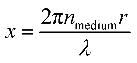 | (1) |
The scattered intensity is also a function of the relative refractive index of the particle, m.
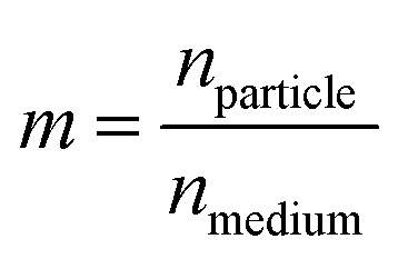 | (2) |
If the refractive index of the medium and the wavelength of incident light is known, the refractive index, nparticle, and radius, r, of the particle can be determined through comparison of the experimental Mie spectrum to an array of Mie spectra calculated using Mie theory, which describes the scattering of electromagnetic light by wavelength-sized spheres.78 Thus, it is assumed that the droplets are spherical and the dispersion of refractive index with wavelength can be described by a dispersion equation. Significant development has been made into methods of retrieving the size and refractive index information from wavelength-resolved scattered light spectra.34,35,71,72,75,79,80 Broadband Light Scattering (BLS) measurements of optically trapped spherical particles involve illumination of the isolated particles with a broad range of wavelengths similar in size to the particle radius, and subsequent collection of the backscattered light over a range of wavelengths and scattering angles.19,74 Although the backscattering of light by single spheres is dominated by the scattering at 180°, integration of the scattered light over a large range of angles relates the intensity of the Mie spectra to a practical collection geometry whilst maintaining the wavelength positions of the MDRs.74 Measuring the scattering of light by the single particles over a large range of wavelengths simultaneously is beneficial for atmospheric studies, as it allows the optical properties of the particle to be determined over a large wavelength range in a single measurement. Additionally, increasing the measured wavelength range increases the number of experimentally observed MDRs, which aids the comparison between experimental and calculated spectra by minimising the number of possible solutions.74 Numerous studies of the optical properties of aerosol have focused on narrow wavelength ranges of <0.05 μm,34,36,38,73,79 with many later techniques using multiple measurement tools to cover a series of wavelength ranges at once,13,16,20,22 in contrast to measuring the scattering over a single broad range.12,19,74,75,77
The primary reason for measuring the scattering of light by atmospheric aerosol particles at UV wavelengths is atmospheric relevance, as it is necessary to fill the current gap in the literature for refractive index dispersions at UV wavelengths of single atmospheric aerosol particles. In this study, the scattering of light by atmospheric aerosol particles is recorded simultaneously over a large UV-visible range of 0.320–0.480 μm, making it a powerful tool to obtain the optical properties of atmospheric aerosol. The procedure to determine the radius and wavelength-resolved refractive index of single aerosol particles is fully detailed in previous work,77 and is similar to other recent literature.14,18,19,35,39,80,81
2 Methods
Atmospheric aerosol particulate matter was collected from various representative atmospheric environments by drawing air through pre-combusted quartz filters. The particulate matter was prepared for optical trapping via extraction with chloroform and water, and stored at −20 °C until required. The extraction process means that the sample can be described as the hydrophobic organic fraction of atmospheric aerosol. Any inorganic compounds that are preferentially soluble in chloroform, will also be in this fraction. A thorough description of the sampling and sample extraction procedures can be found in ref. 23 and 45. Prior to trapping, the atmospheric particulate matter extract was transferred to propan-1-ol suitable for ultrasonic nebulisation, similar to ref. 23. A vertically-aligned counter-propagating optical trap, shown in Fig. 1 and fully detailed in previous work,12 was used to optically trap atmospheric aerosol particles in an aluminium sample chamber. A separate optical system, also shown in Fig. 1, was used to deliver light with a large spectral range from a Laser-Driven Light Source, to illuminate the trapped particle at 90° relative to the trapping direction. The backscattered white light was collected by an UV-optimised objective lens over scattering angles of 150–180°, equivalent to a solid angle of 0.84 sr. The scattered light was delivered via fibre to a spectrograph to produce a Mie spectrum of scattered light intensity as a function of wavelength over wavelengths of 0.299–0.480 μm. Calculated Mie spectra were produced for spheres of known refractive index and radius and compared to the experimental spectra in an iterative fitting process to evaluate the refractive index and radius of the optically trapped spherical aerosol.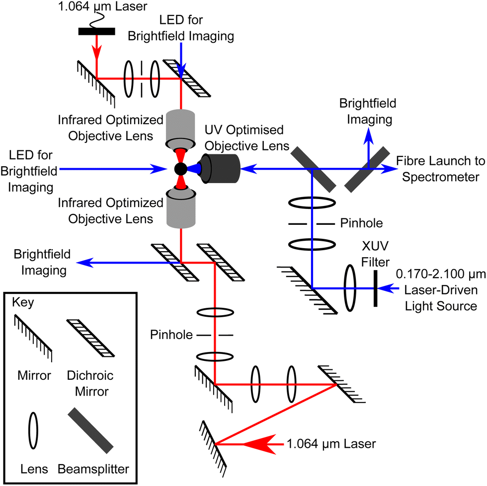 | ||
| Fig. 1 A schematic diagram of the optical trapping and illumination apparatus, not to scale. Infrared laser light (1.064 μm) is focussed through opposing objective lenses to form an optical trap at the sample plane. A broadband light source is delivered through a separate optical system at 90° relative to the optical trap, and the backscattered light is collected and delivered to a spectrograph. | ||
2.1 Sample preparation
Samples were collected and analysed from a location with high anthropogenic aerosol emissions (polluted urban), a location rich in biogenic aerosol emissions (rural forestry), and a location with low anthropogenic emissions but high natural aerosol concentration (remote marine). For each sample, the extraction procedure collects the organic fraction of the samples, to further analyse the optical properties of the organic thin films present on tropospheric aerosol.23,42–44The polluted urban samples were collected over 30 day periods at a height of 20 m, on the Queens Building at the Royal Holloway, University of London (RHUL) campus. This location is within 10 km of three major motorways, London Heathrow airport, and a major urban centre in London, and therefore represents a location with highly anthropogenic emissions.23 The forestry samples were collected in the Straits Inclosure at Alice Holt Forest in south-east England (51°09′ N, 0°51′ W), approximately 60 km from London and managed by Forest Research. A primarily temperate, deciduous forest, the dominant tree species in the Straits Inclosure is mature oak, of which the majority is Quercus robur L., and a minor fraction consists of Q. petraea (Mattuschka) Liebl., and Q. cerris L. Approximately 10% of the tree species are European ash (Fraxinus excelsior L.), and the inclosure contains an additional 4.6 ha of mixed conifers (Pinus nigra subsp. laricio Maire., Pinus sylvestris L., and Cryptomeria japonica (L. f.) D. Don). Below the canopy, the understory contains mostly hazel (Corylus avellana L.), hawthorn (Crataegus monogyna Jacq.), and ground flora.82–88 For each 30 day period, samples were collected on an observation tower at heights of 2 m and 25 m, from the base (in-canopy) and top (above-canopy) of the tower respectively. Collection of aerosol samples at two heights means that an in/above-canopy comparison can be made, and the seasonality of the samples means that the effect of the deciduous trees on aerosol concentrations can be monitored. The remote marine samples were taken at the Sable Island Station on Sable Island, a small Canadian sandbank in the North Atlantic Ocean.89–91 Sable Island is 175 km from the Canadian mainland, and for the purposes of this study acts as a ’background aerosol’ measurement, with high levels of biogenic sea spray emissions49 and minimal anthropogenic emissions from North American continental outflow.56
The atmospheric samples were collected by drawing air through pre-combusted quartz filters (Whatman QM-A Grade/SKC QM-A Grade, 47 mm diameter), which had been placed in a furnace at 500–600° for ≈12 h to remove trace organics. The air was pulled through clean stainless-steel pipelines at a flow rate of 30 L min−1 for the polluted urban samples, and 20–25 L min−1 for the rural forestry and remote marine samples, into a PFA (perfluoroalkoxy) Savillex filter holder. To prevent contamination, the filter holder was dissembled in a glove box, and the sample and filter were stored in the dark at −20 °C until further processing. The extraction procedure used in this study has been detailed in previous publications,23,44,45 and involved full mechanical disintegration of the filter in 10 mL of chloroform (Sigma-Aldrich, ≥99%, contains 0.5–1.0% ethanol as stabilizer) and 10 mL of ultrapure water (>18.2 MΩ cm), before filtration of the resulting solution through a second blank pre-combusted quartz filter (Whatman QM-A Grade/SKC QM-A Grade, 47 mm diameter) to remove any filter debris. The chloroform organic layer, which contained the organic atmospheric extract material, was drawn off into 10 mL amber vials and stored in the dark at −20 °C until further processing. The sample was blown down using dry argon to remove the excess chloroform, and re-dissolved in 2 mL of chloroform for long-term storage in amber glass vials with PTFE lids. The vials were stored in the dark at −20 °C. To be consistent with our previous studies23,44,45 and to ensure that the extract was not hygroscopic only the chloroform extract was used. All glassware and equipment in the extraction procedure was cleaned thoroughly before use with Decon 90 and rinsed extensively with ultrapure water and chloroform. The efficiency of the extraction and re-aerosolisation process were not measured other than to note collection of material over a 30 day period permits capture of several micron-sized droplets in the laboratory at the expense of exhausting the sample. However, the amount of organic material in each sample could be very crudely estimated from the residue left in the glass vial after removal of the chloroform extraction solvent. Concentrated samples, such as the polluted urban samples, commonly left an opaque brown smear on the walls of the glass vial, whereas less abundant samples such as the remote marine and rural forestry samples left extremely faint smears inside the glass vial. To make sure that the amount was sufficient for nebulisation to deliver aerosol particles to the optical trap, the samples were commonly combined into seasons. Details of the constituent months for each sample are included in the ESI.‡ In order to provide a control for the experiment and detect any possible contamination of the samples, blank filters were collected together with each sample. The blank filters were prepared identically to the real samples and travelled with the sampled filters, where they were exposed to the air and immediately sealed for analysis. The blanks were then extracted, and nebulized for optical trapping using the same procedure as for the real atmospheric organic extracts. Several small particles (r < 0.5 μm) were observed in the sample chamber after nebulization of the blanks, which upon trapping underwent rapid losses in droplet volume through evaporation of the propan-1-ol solvent. To further demonstrate that the blank samples contained no material, representative Langmuir trough surface pressure–area isotherms of selected samples are given in the ESI.‡
2.2 Optical trapping
A vertically-aligned counter-propagating optical trap (Fig. 1), was used to optically trap individual atmospheric aerosol particles. The optical trapping system here is detailed in previous work,12 and has been used in numerous recent studies.18,23,24,37,77 Two continuous wave Nd:YAG lasers (Ventus 1064, Laser Quantum) produced 1.064 μm laser beams that were passed through separate beam expansion optics to overfill the back apertures of the opposing objective lenses (Mitutoyo M Plan Apo NIR 50X, NA = 0.42).92 The opposing objective lenses focussed the two laser beams through borosilicate windows to form an optical trap inside an aluminium sample chamber, with a focal offset of ≈10 μm.12 The spatial offset between the optical trapping lasers in the x, y, and z axes was aligned using a piezo-electric stage (Physik Instrumente, E501). The laser powers, which were measured at the point of focus prior to data collection, were set at 15 mW for the downwards beam, and 10 mW for the upwards beam, providing stable trapping and focussed brightfield imaging of the particle.12,24,37,772.3 Aerosol generation
Prior to trapping, the sample was concentrated via gentle evaporation of the chloroform solvent with dry argon and dissolved in 2 mL of propan-1-ol. Propan-1-ol acts as a superior nebulisation carrier solvent to chloroform.23 For the polluted urban aerosol samples, ≈0.33 mL of the atmospheric extract: propan-1-ol solution was added to the chamber of a nebuliser with an additional 2 mL of propan-1-ol. For the remote marine and rural forestry aerosol samples, which contained less particulate matter, additional atmospheric extract was required, and 1 mL of atmospheric extract: propan-1-ol solution was added to the chamber of a nebuliser with an additional 2 mL of propan-1-ol.Prior to nebulisation, gaseous nitrogen was flushed through the entire system for several minutes, including the PTFE-tubing, nebuliser and sample chamber. The flow was regulated using a mass flow meter (MassView MV-302). The nebuliser produced aerosol particles from the atmospheric extract: propan-1-ol solution, and delivered the aerosol via short (≈21 cm) quarter-inch PTFE tubing to the aluminium sample chamber, which contained inlet and exhaust ports in order to maintain a constant gaseous flow throughout the chamber. The nebuliser produced aerosol particles without gaseous flow for ≈30 s, after which the nebuliser was switched off and nitrogen gas was introduced to carry the aerosol particles to the sample chamber. The gaseous flow required to transfer the aerosol to the optical trap whilst maintaining optimal optical trapping ranged from flow rates of ∼30–120 mL min−1. The aerosol particles were initially optically trapped ∼10–50 μm above the borosilicate glass on the bottom of the sample chamber, where the gaseous flow is slower. After optical trapping, the gaseous flow was adjusted to 40 mL min−1 and left for several minutes to allow for any remaining aerosol in the chamber to settle in the sample chamber or leave through the exhaust vent. The aluminium sample chamber was then lowered by ≈5 mm to move the optically trapped particle into the centre of the chamber for optimal spectroscopic imaging. The carrier solvent propan-1-ol evaporates rapidly during transit. The temperature, pressure and humidity in the sample chamber were approximately 20 °C, atmospheric pressure and 35 ± 3.2% respectively, but were not locally controlled beyond the temperature and humidity controlled room. The stability of the optical trap was constant for timescales of several hours.
2.4 Imaging
To identify the presence of a particle in the optical trap and allow for optimisation of the trapping strength, a white LED (Comar 01 LD 555) placed above the upper objective lens provided brightfield imaging. The lower objective lens acted as a condenser to image the trapped particle onto a charge-coupled device (Sony XC-ST51CE CCD), and the stability of the trap was optimised during trapping via adjustment of the focal offset of the two opposing laser beams. The illuminating LED was switched off during data acquisition. In a deviation from previous work,12,14,18,23,37,74 a separate optical system was constructed at 90° relative to the existing optical trap to maximise the illumination of the particle by UV wavelengths (Fig. 1). A Laser-Driven Light Source (ENERGETIQ EQ-99X LDLS) produced broadband light with a very large spectral range (0.170–2.100 μm), which was filtered to remove wavelengths <0.295 μm and focussed onto the trapped aerosol using an UV-optimized, long-working distance objective lens (Thorlabs LMUL-50X-NUV-SP, NA = 0.42). The elastically backscattered light was collected as a function of wavelength by the same objective lens over scattering angles of 150–180°, representing a solid angle of 0.84 sr. The collected light was directed into the 20 μm entrance slit of the spectrometer (Acton SP2500i, 300 groove per mm, 0.300 μm blaze diffraction grating). The spectrometer recorded the intensity as a function of wavelength over a range of ≈0.181 μm from 0.299–0.480 μm, with a resolution of 2.609 × 10⁻⁴ μm at the centre wavelength (λ = 0.390 μm).2.5 Data analysis
A computational program, based on the theoretical methods set out in the BHMIE computational code,78 detailed in ref. 77 and written in Python3.6 compared each experimental Mie spectrum to a series of calculated Mie spectra, to determine the refractive index dispersion and radius of the optically trapped aerosol. The wavelength-dependence of the real refractive index can be described in the visible region by the Cauchy equation: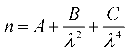 | (3) |
For the polluted urban spring and summer samples, the data were recorded at two separate wavelength ranges. The wavelength ranges were 0.290–0.380 μm and 0.350–0.440 μm, with centre wavelengths of 0.340 and 0.400 μm, and resolutions of 1.291 × 10⁻⁴ μm and 1.285 × 10⁻⁴ μm respectively. The UV 0.340 μm centre wavelength spectrum contained a larger number of sharp, defined MDRs, and so the UV spectra were used to determine the refractive index dispersion and radius of the particle, using the automated fitting process. For the remote marine samples and the rural forestry above canopy spring sample, the small particle sizes (<0.6 μm) resulted in Mie scattering spectra with ≤5 broad MDRs, which cannot be fit accurately using the automated fitting process (see ESI‡). A manual fitting process, similar to that of the automated fitting process, was used in order to determine the size and refractive index dispersion of the small particles. An optimal fit between the experimental Mie spectrum and calculated Mie spectra was determined by minimising the difference in the wavelength positions of the MDRs across the spectrum. Crucially in the manual fitting process, the comparison involved consideration of the overall shapes of the experimental and calculated Mie spectra. The associated errors with the manual fitting process are significantly increased and are discussed in Section 3.1.
2.6 Atmospheric radiative-transfer modelling
It is instructive to assess if the experimental results of the work presented here may be important to the light scattering in the atmosphere. Thus the experimental results of the work were applied to a 1D radiative-transfer model to assess the impact that organic films, i.e. the materials studied, coating mineral aerosol may have on top of atmosphere albedo as a function of organic film thickness. Mineral aerosol were chosen as the core as Jones et al.18 have previously demonstrated that organic compounds can form core–shell aerosol on silica particles. The aerosol particles were considered spherical for ease of calculation. The assessment was performed for remote and urban aerosol films to bracket typical atmospheric conditions. An atmospheric radiative-transfer model93 was applied to study an atmospheric aerosol layer consisting of core mineral aerosol coated in an organic shell with the real refractive index of the atmospheric aerosol extract measured within the work presented here and Shepherd et al.23 and with imaginary refractive index data from wider literature. The change in the top-of-the-atmosphere albedo was calculated for an aerosol layer with the composition of a silica core aerosol surrounded by a shell of urban, or remote atmospheric aerosol extract with the film thickness varying from 10−4–0.1 μm. The silica core aerosol had a size distribution of atmospheric aerosol typical of remote and urban environments.94 The change in the top-of-the-atmosphere albedo is reported similar to the approach of Shepherd et al.23 Note these calculations are an exploratory study to simply demonstrate potential effects on the top-of-the-atmosphere albedo owing to the presence of organic film with refractive indexes measured herein on pure core–shell particles in the atmosphere versus no organic film (i.e. core only).The atmospheric radiative-transfer model uses the DISORT code (e.g.93) in TUV.95 The model uses values of the scattering, absorption, and asymmetry parameter of aerosols to calculate the change in solar radiation through the atmosphere. To calculate the scattering and absorption parameters for coated spheres, Mie calculations were performed for the core–shell particles using BHCOAT, a code developed and described by Bohren and Huffman.78 Scattering, absorption, and asymmetry parameter for the particle are calculated from the refractive index of the core and shell. For all aerosol particles, the refractive index of the core is a wavelength-dependent value for silica,96,97 and the refractive index of the surrounding medium is a wavelength-independent value for air of 1.00–0.0i. The shell of the aerosol has a wavelength-dependent refractive index of the urban, or remote aerosol extracts, from the work presented here and Shepherd et al.23 The absorption properties of the woodsmoke aerosol extract were included in the calculation and based on a wavelength dependent complex refractive index calculated from previous studies (Kirchstetter et al.;98 Shepherd et al.;23 Virkkula et al.99).
The core–shell Mie calculation was used to obtain scattering and absorption cross sections and asymmetry parameters for particles averaged over a trimodal aerosol core size distribution94 over wavelengths covering 0.320–0.785 μ m. The remote and urban size distributions were used accordingly from Jaenicke94 from a radius of 0.01–1 μm. The ground albedo was set to 0.1. Aerosol was placed in three consecutive 1 km thick layers at the surface, forming a 3 km thick aerosol layer. The aerosol optical depth for each of these layers was set to 0.235, and an Elterman aerosol profile was present in the rest of the atmosphere with no cloud was placed in any subsequent layers. The solar zenith angle was set at 60°. The albedo of the top of the atmosphere was calculated as the ratio of incoming to outgoing irradiance at 80 km altitude. Calculations were also performed for the same aerosol with no film. The difference in top of atmosphere albedo (ΔAlbedo) was then calculated by subtracting the albedo without an organic film from the albedo with organic film.
3 Results and discussion
Fig. 2 shows representative experimental and best-fit calculated Mie spectra from the urban, forestry and remote marine sampling locations in this study. The variability in the intensity and number of MDRs in each spectrum in Fig. 2 is a consequence of the varying sizes and refractive index dispersions, and the details for the individual spectra in Fig. 2 are included in Table 1. The uncertainties in A and nλ=0.35μm (1 significant figure) in Table 1 are included for samples where more than one repeat was undertaken, representing the average value and the uncertainty from two standard deviations over the repeat measurements. The Cauchy coefficients B and C are partially correlated, and the uncertainty in these coefficients is not reported. The given uncertainties in the radius (1 significant figure) are from the automated (r ± 0.001) and manual (r ± 0.005) fitting processes. After the droplet scattering was measured, each droplet was deposited onto the lower surface of the sample chamber. In all cases, the droplets spread onto the surface, indicating that the extracted real organic material from the aerosol samples formed spherical liquid droplets which remained liquid throughout the experiments. Other studies have demonstrated significant photodegradation of optically trapped aerosol particles containing fatty acids in spectroscopic experiments.19,100 In this study, no photochemical effects were observed that resulted in a shifting of the refractive index. Table 2 contains the determined values of the refractive index dispersion, the range in particle radii studied for each sample, and the values of the refractive index at 0.35 μm, for all samples investigated in this work. The given uncertainties in A and nλ=0.35μm (1 significant figure) are calculated in the same process as for Table 1, and the uncertainty in the radii ranges from the automated (r ± 0.001) and manual (r ± 0.005) fitting processes are not included.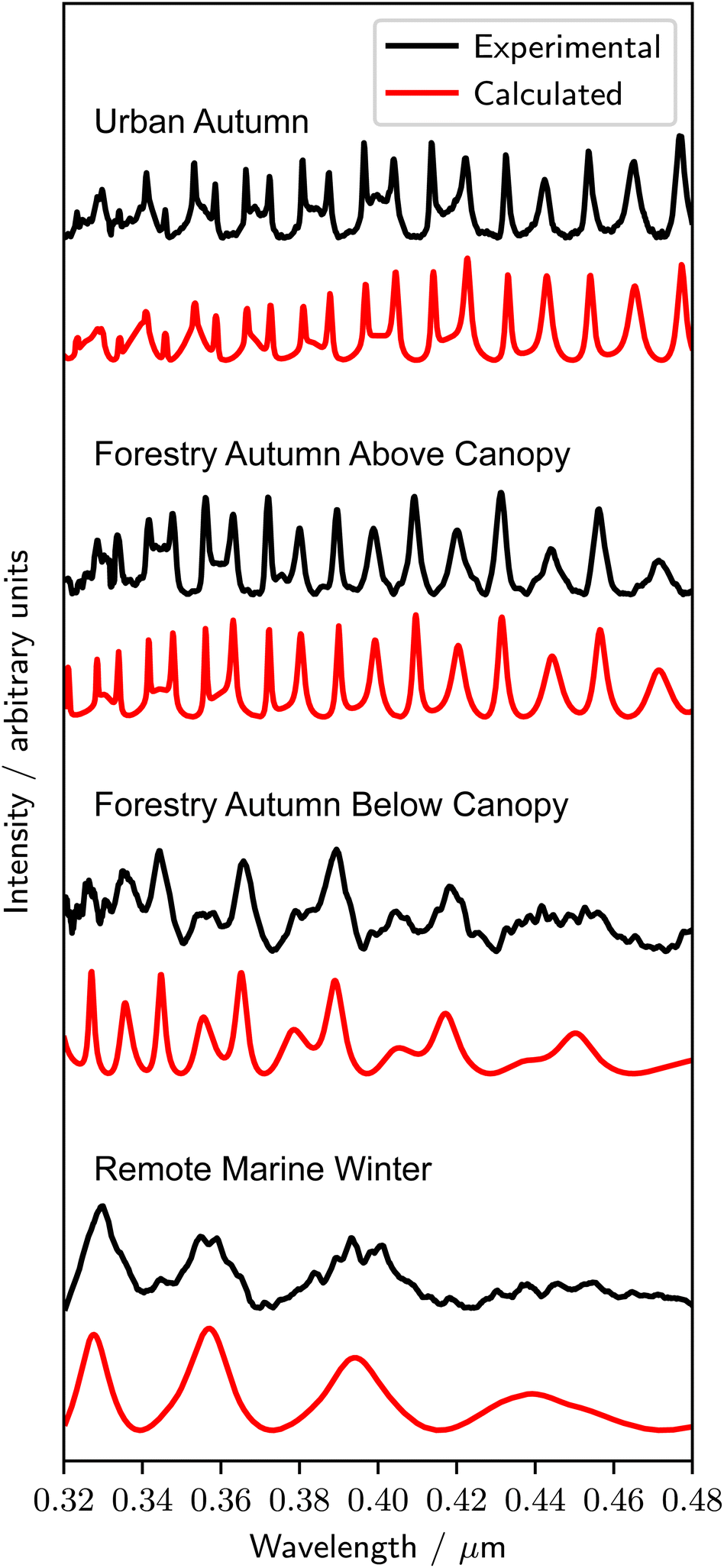 | ||
| Fig. 2 A representative experimental Mie spectrum for each sampling location in this study, with the associated best-fit calculated spectrum obtained through the automatic Python fitting process. | ||
| Sample | Season | A | B (μm2) | C (μm4) | Radii (μm) | n λ=0.35μm |
|---|---|---|---|---|---|---|
| Polluted urban | Autumn | 1.451 ± 0.005 | 1.18 × 10⁻³ | 2.27 × 10⁻⁴ | 1.091 ± 0.001 | 1.476 ± 0.001 |
| Forestry above canopy | Autumn | 1.457 ± 0.02 | 9.05 × 10⁻⁴ | 2.76 × 10⁻⁴ | 0.930 ± 0.001 | 1.482 ± 0.003 |
| Forestry below canopy | Autumn | 1.437 | 3.77 × 10⁻³ | 6.11 × 10⁻⁴ | 0.645 ± 0.005 | 1.508 |
| Remote marine | Winter | 1.429 ± 0.03 | 1.00 × 10⁻³ | 1.00 × 10⁻⁴ | 0.475 ± 0.005 | 1.444 ± 0.007 |
| Sample | Repeats | A | B (μm2) | C (μm4) | Radii (μm) | n λ=0.35μm |
|---|---|---|---|---|---|---|
| Remote marine autumn | 1 | 1.416 | 2.00 × 10⁻³ | 1.50 × 10⁻⁴ | 0.463 | 1.442 |
| Remote marine winter | 2 | 1.419 ± 0.03 | 2.00 × 10⁻³ | 1.00 × 10⁻⁴ | 0.475, 0.485 | 1.442 ± 0.007 |
![[thin space (1/6-em)]](https://www.rsc.org/images/entities/char_2009.gif) |
||||||
| Forestry below canopy autumn | 1 | 1.437 | 3.77 × 10⁻³ | 6.11 × 10⁻⁴ | 0.645 | 1.508 |
|
||||||
| Forestry above canopy spring | 1 | 1.455 | 5.00 × 10⁻⁴ | 5.00 × 10⁻⁵ | 0.542 | 1.462 |
| Forestry above canopy summer | 3 | 1.443 ± 0.01 | 5.46 × 10⁻⁴ | 2.68 × 10⁻⁴ | 0.749–0.889 | 1.465 ± 0.01 |
| Forestry above canopy autumn | 3 | 1.448 ± 0.02 | 2.78 × 10⁻³ | 1.63 × 10⁻⁴ | 0.795–0.978 | 1.481 ± 0.003 |
|
||||||
| Polluted urban spring | 2 | 1.403 ± 0.03 | 4.91 × 10⁻³ | 6.11 × 10⁻⁶ | 0.772, 0.775 | 1.444 ± 0.03 |
| Polluted urban summer | 2 | 1.458 ± 0.007 | 1.79 × 10⁻³ | 1.66 × 10⁻⁴ | 0.671, 0.780 | 1.483 ± 0.02 |
| Polluted urban autumn | 3 | 1.452 ± 0.005 | 7.70 × 10⁻⁴ | 2.49 × 10⁻⁴ | 0.829–1.144 | 1.475 ± 0.001 |
| Polluted urban winter | 2 | 1.457 ± 0.00004 | 1.84 × 10⁻³ | 1.88 × 10⁻⁴ | 0.789, 0.895 | 1.485 ± 0.003 |
In the work presented here the Cauchy dispersion equation has been shown to fit the experimental data for a weakly absorbing material in the near UV region. The Cauchy equation is normally replaced with the Sellmeier equation for fitting the refractive index over wavelengths where the either the real or imaginary part of the refractive index may be changing quickly (i.e. absorption) at specific wavelength or wavelengths. Previously Shepherd et al.23 have demonstrated that the Cauchy equation is suitable for organic materials in the visible, using woodsmoke and humic acid samples. Shepherd et al.23 also show that the absorption in these samples was significant and affected the intensity of the Mie spectra measured in the experiment, but not the wavelength of the peaks used to determine the real component of the refractive index dispersion. The applicability of the Cauchy dispersion equation to represent the absorbing samples of Shepherd et al.23 and those presented here may stem from these samples being mixtures of many similar molecules and the values of A, B, and C determined actually representing an average of the Cauchy coefficient of many different molecules. The imaginary component of refractive index used to match the calculated Mie spectral intensities to the measured intensities shown in Fig. 2 are presented in ESI.‡
3.1 Error analysis
Multiple droplets were analysed for each sample, however low amounts of organic material in several of the samples meant that only small particles (r < 0.4 μm) could be trapped. Mie spectra of small particles contain weak, broad MDRs which cannot be accurately compared to calculated Mie spectra, and so several samples contain only one repeat. For samples with two or more repeats, the determined values of the Cauchy coefficient, A, and the refractive index at 0.35 μm are reported as the average ± two standard deviations between the repeats (Table 2). It should be noted that the polluted urban autumn and winter aerosol samples and the rural forestry summer and autumn above-canopy aerosol samples each had between 12 and 23 MDRs in each spectrum, and multiple repeats for each sample, resulting in lower uncertainties in the refractive index of ≤0.01. The low errors for these samples demonstrate the accuracy of this technique when studying concentrated aerosol samples with many MDRs across the Mie spectrum, and validates the move to UV wavelengths to increase the number of MDRs.The automated fitting process, which determined the optimal radius through minimising the value of the fitting coefficient, δ, (see ESI‡). The fitting routine involved a multi-stage process with a wide search of 10201 calculated Mie spectra over a 500 nm radius range, and then a more detailed search of 25410 calculations across a narrower 12 nm radius range. An example of a typical plot of r vs. δ is included in the ESI,‡ and is characterized by linear trends approaching the optimal radius from higher and lower radii. The linear trends of six typical experimental data sets of r vs. δ were analysed using the least squares method, and the two standard deviation errors in each trend were used to estimate the two standard deviation uncertainty in the optimal radius from the automated fitting process. The uncertainty in the radius and corresponding uncertainty in the refractive index from the automated fitting process were therefore estimated to be ±0.001 μm and ±0.002 respectively.
For samples fit using the manual fitting process, which includes all remote marine samples and the above canopy spring rural forestry sample, the uncertainty in determined radius and refractive index is significantly larger, and was estimated by adjusting r from the best fit by 0.001 μm, and adjusting A to realign the fit between the experimental and calculated data. The largest and smallest radii at which the spectrum could no longer be reliably reproduced through an adjustment of A was used to determine the uncertainty in the manual fitting process. The uncertainty in radius and refractive index for the manually fit samples was determined to be 0.005 μm and 0.02 respectively.
3.2 Remote marine aerosol
The monthly remote marine samples were combined into three month seasons owing to low amounts of extracted organic material, of which only autumn and winter produced particles of a sufficient size to result in Mie spectra with enough defined MDRs for accurate determination of the particle's optical properties. Literature studies of the refractive index dispersion with wavelength of remote marine aerosol are rare, and so our results have been compared to remote aerosol measurements from different environments. Our results, shown in Fig. 3, are consistent with literature measurements of Antarctic aerosol,23,26 and significantly higher than measurements of Hawaiian aerosol.25 No seasonality can be observed in the refractive index dispersions with wavelength, with similar results observed for autumn and winter months.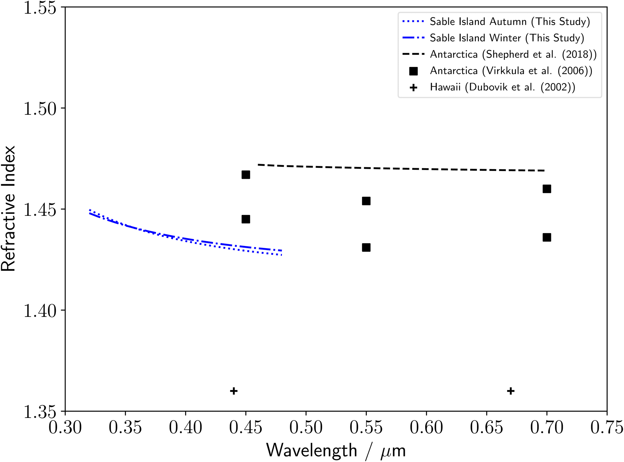 | ||
| Fig. 3 Comparison of the remote marine aerosol refractive index dispersions determined in this study to a series of literature measurements, including refractive index dispersions of remote Antarctic aerosol23,26 and remote marine Hawaiian aerosol.25 | ||
3.3 Forestry aerosol
The determined refractive index values for rural forestry aerosol from Alice Holt Forest are shown in Fig. 4. For the above-canopy aerosol samples, the dispersion of refractive index with wavelength are similar for spring and summer, with a notable increase across all wavelengths in autumn. The relative refractive indices of aerosol either above or inside the forestry canopy can be made by comparing the aerosol samples taken in autumn at observation tower heights of 25 and 2 m. The in-canopy forestry aerosol sample was observed to have a much higher refractive index at the lowest studied wavelengths, and an increased dependence of the refractive index on wavelength compared to the above canopy forestry aerosol sample. A summary of the current literature for the refractive indices of biogenic organic atmospheric aerosol species is included in Fig. 4. It should be noted that the majority of the literature measurements in Fig. 4 are for studies of distributions of aerosol particles inside a chamber, rather than investigations of single aerosol particles as in this study. There are two exceptions to this, where either thin films of monoterpene derived compound were investigated,11 or the study104 computationally calculated the refractive index of α-pinene derived SOA. There is a significant variation in the literature values of the refractive index for biogenic organic atmospheric aerosol, with most values over near-UV to visible wavelengths of 0.35–0.70 μm falling between 1.4–1.6. The measurements in this study are all within this literature range, and the results agree especially well with the values of ref. 15, 16 and 22. The upper and lower refractive index dispersions with wavelength from ref. 22 in Fig. 4 are for β-pinene derived SOA, after exposure to OH radicals for 0.5 and 12.4 days respectively. The dispersions in this study, and in particular the autumn above-canopy sample, are close to the value in ref. 22 for OH radical exposure over 12.4 days, which may indicate significant atmospheric ageing of our samples. In addition, our results are noticeably lower than that reported11 in the study of thin films of monoterpene derived compounds, rather than aerosol particles.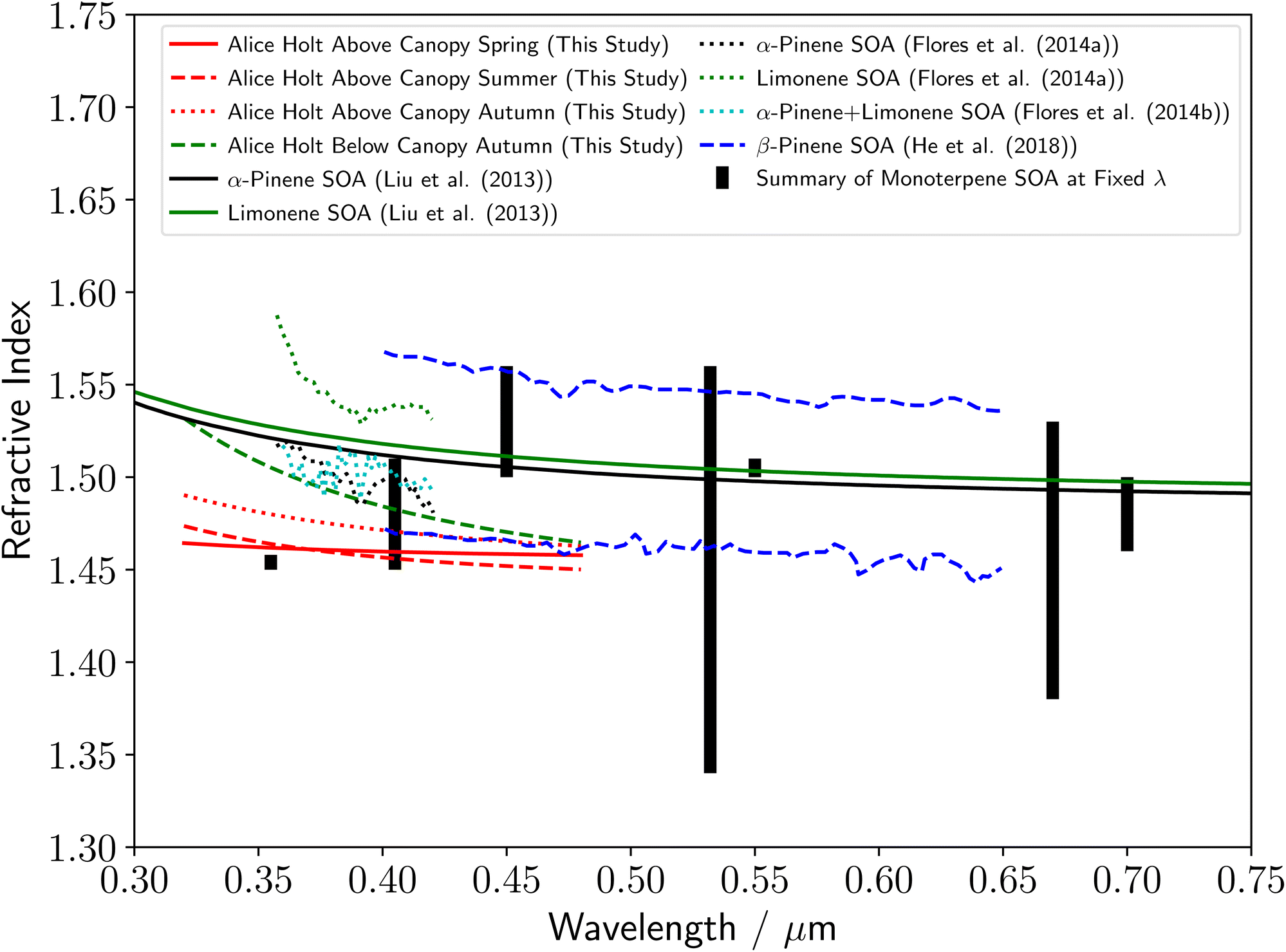 | ||
| Fig. 4 Comparison of the rural forestry aerosol refractive index dispersions with wavelength determined in this study to a series of literature measurements of monoterpene derived SOA refractive index values, including α-pinene SOA,11,15 β-pinene SOA (upper line from 12.4 days collection and lower line from 0.5 days collection),22 Limonene SOA,11 and an α-pinene/limonene SOA mixture.16 The thick black lines demonstrate a summary of literature refractive index measurements of monoterpene-derived SOA at single wavelengths.27,28,30,101–109 The change in y-axis compared to Fig. 3 should be noted. | ||
3.4 Polluted urban aerosol
Fig. 5 displays the determined refractive index dispersions with wavelength for polluted urban aerosol from RHUL in this study. The values are similar for summer and winter, with a small decrease in refractive index in autumn and a much larger decrease in refractive index in spring. A summary of the current literature for the refractive indices of AVOC derived SOA over near-UV to visible wavelengths is included in Fig. 5, where the majority of the literature refractive indices are for chamber-based measurements. Literature values for the refractive index for AVOC derived SOA vary between 1.43–1.66 over near-UV to visible wavelengths of 0.35–0.70 μm, and apart from the spring aerosol sample, our results lie at the lower region of the literature range. The refractive index dispersions with wavelength from ref. 23 use a similar single-particle optical trapping technique as in this study but with a spectroscopic system optimized for visible wavelengths. Shepherd et al.23 studied aerosol samples collected in 2015–2016 from the same urban sampling location at RHUL. The samples in this work were collected in 2017–2019. The urban environmental conditions are uncontrolled and may present year-to-year variability. The possibility of a bias in systematic uncertainties has been assessed using polystyrene beads as a reference. Mie scattering spectra from the same bead was captured in a dual set-up optical configuration that combines the collection technique described here and from previous work.23 The different techniques show no systematic variation (see ESI‡). In addition, parameters such a spectrometer calibration, polarisation, collection cone angle, spectrometer slit width and baselining were also assessed for bias. As was true for the rural forestry samples, our results are in good agreement with refractive index values from previous studies.16,22,30 Flores16 studied SOA produced from a mixture of biogenic and anthropogenic precursors throughout ageing with OH, and our results agree well with those associated with minimal ageing. The upper and lower refractive index dispersions with wavelength from ref. 22 in Fig. 5 are for p-xylene derived SOA, after exposure to OH radicals for 0.5 and 12.4 days respectively. In contrast to the comparison of our results to Flores,16 our results agree well with the data from ref. 22 for significantly aged aerosol. As was true for the rural forestry samples, the polluted urban refractive index dispersions with wavelength are noticeably lower than that reported in the study,11 of thin films of catechol.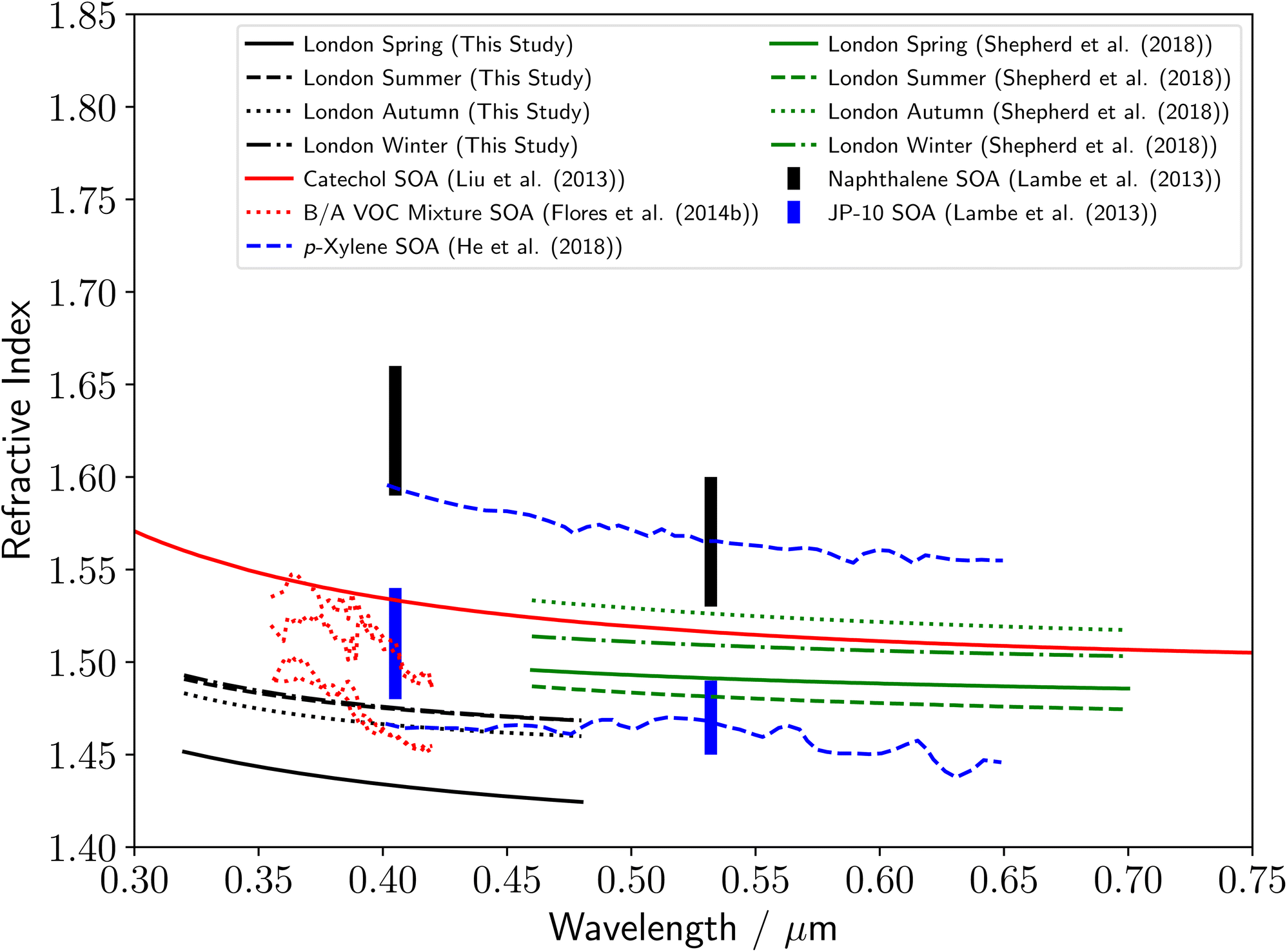 | ||
| Fig. 5 Comparison of the polluted urban aerosol refractive index dispersions determined in this study to a series of literature measurements of refractive index dispersions of SOA derived from anthropogenic sources, including refractive index dispersions for catechol SOA,11 biogenic/anthropogenic mixtures of α-pinene + limonene + p-xylene-d10 SOA throughout ageing with OH16 and p-xylene SOA throughout ageing with OH.22 The seasonal values in green are from a previous study over visible wavelengths at the same sampling location at RHUL.23 The capped lines demonstrate a summary of literature refractive index measurements of naphthalene (black) and tricyclo[5.2.1.02,6]decane, referred to as JP-10 (blue) SOA at single wavelengths.30 The change in y-axis compared to Fig. 4 should be noted. | ||
3.5 Overview
Utilizing the literature measurements in Fig. 3–5, the range of measured literature values of the real refractive index for atmospheric organic aerosol over near-UV to visible wavelengths of 0.35–0.70 μm tends to increase from remote marine (≈1.36–1.47), to rural forestry (≈1.40–1.60), to polluted urban (≈1.43–1.66) environments.23 Redmond and Thompson,104 outline the parameters, such as chemical properties, that could account for the observed changes in refractive index. A summary of the refractive index dispersions with wavelength observed in this study are given in Fig. 6. Our results are in agreement with this trend for the remote marine samples from Sable Island, which were determined to have the lowest refractive index dispersions with wavelength of any studied environment (Table 2 and Fig. 6). In addition, the spring polluted urban sample was observed to have an unusually low refractive index, close to that of the remote marine aerosol, indicating that the spring polluted urban sample may have been relatively clean in comparison to the other seasonal polluted urban samples. In contrast to the observed literature trend in Fig. 4 and 5, our results demonstrate similar ranges of refractive index for above-canopy rural forestry and polluted urban aerosol samples, indicating that biogenic and anthropogenic aerosol have similar light scattering properties. Further studies will be needed to understand these differences in more detail. There was insufficient sample to run a series of analytical tests, however the refractive index can be linked to chemical properties of atmospheric aerosol such as degree of unsaturation, polarizability, mass density and molecular weight.104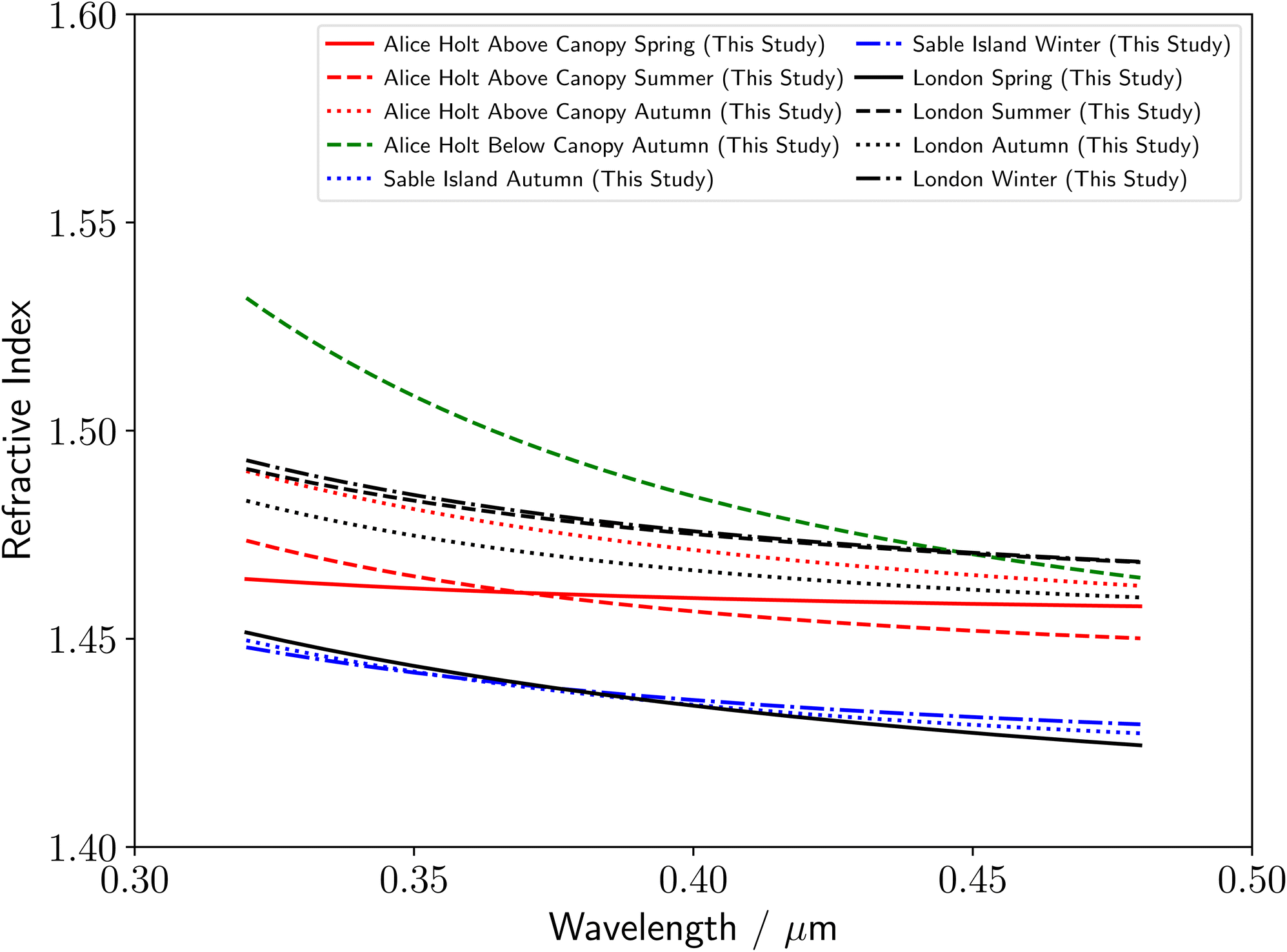 | ||
| Fig. 6 Comparison of all real components of the refractive index measured in this study: forestry atmospheric aerosol extracts from Alice Holt Forest above (red) and below (green) the canopy, remote marine atmospheric aerosol extracts from Sable Island (blue) and urban atmospheric aerosol extracts from RHUL (black). | ||
Throughout this study, the Cauchy equation was assumed to be sufficiently accurate in approximating the real refractive index dispersion of each aerosol sample. This was found to be accurate throughout the study, with the fitting process able to determine a Cauchy-based refractive index dispersion for all studied samples. This therefore demonstrates that for tropospheric aerosol, the Cauchy dispersion formula is applicable to describe the refractive index for the full range of visible and near-UV wavelengths. Several studies have previously measured the refractive index dispersion at wavelengths below 0.350 μm, for atmospheric aerosol species from commercial sources, using spectroscopic ellipsometry to study thin films of monoterpene derived secondary organic aerosol,11 and, optical trapping and BLS to study single polystyrene latex spheres, and droplets of glycerol, aqueous potassium carbonate, and oleic acid.19 The experiment detailed here represents the first single-particle measurements of the refractive index dispersion of real aerosol organic material extracted from the atmosphere below 0.350 μm, extending the literature towards the UV tropospheric wavelength limit at the Earth's surface. In addition, Fig. 6 shows that comparing the real refractive index dispersion of atmospheric aerosol particles over near-ultraviolet wavelengths (where the refractive index increases rapidly with decreasing wavelength) gives additional insights into locational and seasonal changes in the refractive index dispersion.
4 Atmospheric implications
Aerosols influence planetary albedo by altering the ratio of light scattered and absorbed as it passes through the atmosphere.10 Changes to these aerosol, such as the introduction of an organic film, can cause changes to the optical and physical properties of these aerosol23,44,101 consequently influencing their effect on planetary albedo. The development and oxidation of organic films on tropospheric aerosol represent a dynamic environment of changing structural and optical properties of aerosol that may play a significant role in aerosol forcing effects. These properties vary significantly between environments and as such any consideration of interactions and changes to aerosol-climate effects should be environment-dependent. This study takes the observed real refractive indexes of polar and urban organics and combines these with existing literature to produce an example of the influence of organic coated mineral aerosols on planetary albedo in these environments for the organic species studied in the work presented here. Fig. 7 demonstrates the impact of an organic film of a given environment (remote or urban), and thickness of that film, on the top-of-the-atmosphere albedo (henceforth albedo) as calculated by a 1-dimension radiative-transfer model. The presence of an organic film typically causes a decrease in albedo except for the very thinnest urban films considered (<10−3 μm) at shorter wavelengths (<0.500 μm). The albedo decreases with increasing film thickness with the largest change for increasing thinner films as opposed to increasing thicker films. The albedo of the films associated with remote and urban environments have different responses with increasing thickness owing to the interplay between light absorption and light scattering convoluted by increasing particle size. The change in albedo owing to a thin urban film decreases quickly with film thickness relative to a remote film. Note the two size distributions are different. The urban film is a more light absorbing film than the remote film. Comparison of the albedo for the remote film at a wavelength of 0.320 μm (light absorbing) relative to a wavelength of 0.500 μm (light scattering dominated) with film thickness demonstrates different behaviours.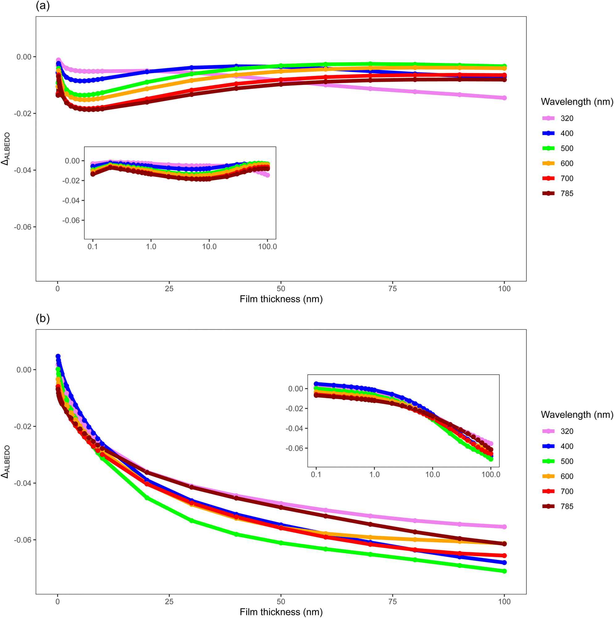 | ||
| Fig. 7 The change in the top-of-atmosphere albedo from a 1D radiative-transfer model for a layer of spherical silica aerosol with and without an organic film as a function of film thickness. The distribution of particle size and the optical properties of the films are described in the text. (a) The change in albedo for an atmospheric layer of aerosol with remote size distribution and optical properties consistent with remote aerosol. (b) The change in albedo for an atmospheric layer of aerosol with urban size distribution and optical properties consistent with urban aerosol. | ||
Throughout an aerosol particle's lifetime organic films may form, thicken, and be removed by oxidation in the atmosphere, and thus the structure and optical properties of these aerosol will vary with both time, source and environment. The results shown in this work demonstrate that even a thin organic film, such as those studied inn the work presented here of ∼10−4 μm can have atmospherically relevant impacts.
5 Conclusions
Optical trapping was combined with a bespoke UV-optimised BLS system to investigate the refractive index dispersions of atmospheric aerosol samples from a range of tropospheric environments. Tropospheric aerosol samples were collected on quartz filters at remote marine (Sable Island), deciduous forestry (Alice Holt Forest) and polluted urban (London) locations, and the organic fraction of the collected aerosol was extracted and nebulized for optical trapping of single aerosol particles for further spectroscopic analysis. All particles were observed to form spherical liquid particles, and the backscattered light from the optically trapped aerosol particles was collected over scattering angles of 150–180° to produce Mie scattering spectra of intensity as a function of wavelength. The experimental spectra were compared to spectra calculated using Mie theory to characterize the radius and refractive index dispersion with wavelength of the aerosol to precisions of 0.001 μm and 0.002 respectively. Refractive index values of tropospheric aerosol samples from marine, forestry and urban environments are consistent with those calculated when using a Cauchy dispersion equation over a large UV-visible wavelength range of 0.320–0.480 μm, demonstrating an extension of the applicability of the Cauchy equation to wavelengths below 0.350 μm. In addition, single-particle measurements of the real refractive index dispersions with wavelength of aerosol particles from real organic tropospheric extracts are demonstrated for the first time below 0.350 μm. The refractive index values increased from remote marine aerosol (n = 1.442 (λ = 0.350 μm)) to forestry above canopy aerosol (n = 1.462–1.481 (λ = 0.350 μm)) and polluted urban aerosol (n = 1.444–1.485 (λ = 0.350 μm)), to forestry below canopy aerosol (n = 1.508 (λ = 0.350 μm)). Seasonal changes in the refractive index were observed for the forestry and urban samples, overall demonstrating that the refractive index of atmospheric aerosol particles is dependent on the sampling environment, and varies seasonally. The regional variation in the optical properties of organic films and how these films develop and decay over their lifetimes may play a significant role in determining the true forcing effect of aerosols on our atmosphere. Even a very thin film of ∼10−4 μm can have atmospherically relevant impacts from starkly different source environments.Author contributions
MK and AW (STFC) designed the experiment and assisted CB throughout the data collection. MK collected the urban aerosol filter samples, MK and MW collected the forestry aerosol filter samples, AW and GL (ECCC) collected the remote marine aerosol filter samples. MK and CB extracted the samples into chloroform. AW (STFC) designed and aligned the optical trapping system, and CB assisted with optical trapping alignment throughout. EJS led the atmospheric implications, its associated methodology, and the modelling and analyses contained therein were primarily authored, with aid of BW and MK. CB designed, constructed and aligned the UV spectroscopy system. CB performed the experiment with assistance from MP, MK and AW (STFC). CB analysed and interpreted all of the collected data, and the manuscript was written by CB with inputs from all authors.Conflicts of interest
There are no conflicts to declare.Acknowledgements
The authors would like to thank STFC and the Central Laser Facility for access to equipment funded under App. No. 19230006 and 20230019 and Programme Access no. 1832, NERC for support under Grant No. NE/T00732X/1, and Royal Holloway, University of London for funding Connor Barker's PhD studies. We would also like to thank Megan McGrory for access to the Python code used for Mie spectra fitting in this study. We are grateful to Gina Little (Environment and Climate Change Canada) for logistics on Sable Island.Notes and references
- U. Pöschl, Angew. Chem., Int. Ed., 2005, 44, 7520–7540 CrossRef PubMed.
- O. Boucher, D. Randall, P. Artaxo, C. Bretherton, G. Feingold, P. Forster, V.-M. Kerminen, Y. Kondo, H. Liao, U. Lohmann, P. Rasch, S. Satheesh, S. Sherwood, B. Stevens and X. Zhang, in Climate Change 2013 the Physical Science Basis: Working Group I Contribution to the Fifth Assessment Report of the Intergovernmental Panel on Climate Change, ed. T. Stocker, D. Qi, G.-K. Plattner, M. Tignor, S. Allen, J. Boschung, A. Nauels, Y. Xia, V. Bex and P. Midgley, Cambridge University Press, Cambridge, United Kingdom, 2013, ch. 7, pp. 571–658 Search PubMed.
- T. Moise, J. M. Flores and Y. Rudich, Chem. Rev., 2015, 115, 4400–4439 CrossRef CAS PubMed.
- A. Valenzuela, J. P. Reid, B. R. Bzdek and A. J. Orr-Ewing, J. Geophys. Res.: Atmos., 2018, 123, 6469–6486 CrossRef.
- J. H. Seinfeld and S. N. Pandis, Atmospheric Chemistry and Physics: from Air Pollution to Climate Change, John Wiley & Sons, New York, 2nd edn, 2006 Search PubMed.
- Atmospheric Science for Environmental Scientists, ed. C. N. Hewitt and A. V. Jackson, John Wiley & Sons, Chichester, 2009 Search PubMed.
- N. Meskhidze, M. D. Petters, K. Tsigaridis, T. Bates, C. O'Dowd, J. Reid, E. R. Lewis, B. Gantt, M. D. Anguelova, P. V. Bhave, J. Bird, A. H. Callaghan, D. Ceburnis, R. Chang, A. Clarke, G. de Leeuw, G. Deane, P. J. Demott, S. Elliot, M. C. Facchini, C. W. Fairall, L. Hawkins, Y. Hu, J. G. Hudson, M. S. Johnson, K. C. Kaku, W. C. Keene, D. J. Kieber, M. S. Long, M. Mårtensson, R. L. Modini, C. L. Osburn, K. A. Prather, A. Pszenny, M. Rinaldi, L. M. Russell, M. Salter, A. M. Sayer, A. Smirnov, S. R. Suda, T. D. Toth, D. R. Worsnop, A. Wozniak and S. R. Zorn, Atmos. Sci. Lett., 2013, 14, 207–213 CrossRef.
- B. H. Samset, G. Myhre and M. Schulz, Nat. Clim. Change, 2014, 4, 230–232 CrossRef.
- G. Myhre, W. Aas, R. Cherian, W. Collins, G. Faluvegi, M. Flanner, P. Forster, Ø. Hodnebrog, Z. Klimont, M. T. Lund, J. Mülmenstädt, C. Lund Myhre, D. Olivié, M. Prather, J. Quaas, B. H. Samset, J. L. Schnell, M. Schulz, D. Shindell, R. B. Skeie, T. Takemura and S. Tsyro, Atmos. Chem. Phys., 2017, 17, 2709–2720 CrossRef CAS.
- P. Arias, N. Bellouin, E. Coppola, R. Jones, G. Krinner, J. Marotzke, V. Naik, M. Palmer, G.-K. Plattner, J. Rogelj, M. Rojas, J. Sillmann, T. Storelvmo, P. Thorne, B. Trewin, K. A. Rao, B. Adhikary, R. Allan, K. Armour, G. Bala, R. Barimalala, S. Berger, J. Canadell, C. Cassou, A. Cherchi, W. Collins, W. Collins, S. Connors, S. Corti, F. Cruz, F. Dentener, C. Dereczynski, A. D. Luca, A. D. Niang, F. Doblas-Reyes, A. Dosio, H. Douville, F. Engelbrecht, V. Eyring, E. Fischer, P. Forster, B. Fox-Kemper, J. Fuglestvedt, J. Fyfe, N. Gillett, L. Goldfarb, I. Gorodetskaya, J. Gutierrez, R. Hamdi, E. Hawkins, H. Hewitt, P. Hope, A. Islam, C. Jones, D. Kaufman, R. Kopp, Y. Kosaka, J. Kossin, S. Krakovska, J.-Y. Lee, J. Li, T. Mauritsen, T. Maycock, M. Meinshausen, S.-K. Min, P. Monteiro, T. Ngo-Duc, F. Otto, I. Pinto, A. Pirani, K. Raghavan, R. Ranasinghe, A. Ruane, L. Ruiz, J.-B. Sallée, B. Samset, S. Sathyendranath, S. Seneviratne, A. Sörensson, S. Szopa, I. Takayabu, A.-M. Tréguier, B. van den Hurk, R. Vautard, K. von Schuckmann, S. Zaehle, X. Zhang and K. Zickfeld, in Climate Change 2021: The Physical Science Basis. Contribution of Working Group I to the Sixth Assessment Report of the Intergovernmental Panel on Climate Change, ed. V. Masson-Delmotte, P. Zhai, A. Pirani, S. Connors, C. Péan, S. Berger, N. Caud, Y. Chen, L. Goldfarb, M. Gomis, M. Huang, K. Leitzell, E. Lonnoy, J. Matthews, T. Maycock, T. Waterfield, O. Yelekçi, R. Yu and B. Zhou, Cambridge University Press, Cambridge, United Kingdom and New York, NY, USA, 2021, pp. 33–144 Search PubMed.
- P. Liu, Y. Zhang and S. T. Martin, Environ. Sci. Technol., 2013, 47, 13594–13601 CrossRef CAS PubMed.
- S. H. Jones, M. D. King and A. D. Ward, Phys. Chem. Chem. Phys., 2013, 15, 20735–20741 RSC.
- R. A. Washenfelder, J. M. Flores, C. A. Brock, S. S. Brown and Y. Rudich, Atmos. Meas. Tech., 2013, 6, 861–877 CrossRef.
- S. H. Jones, M. D. King and A. D. Ward, Proc. SPIE 9164, Optical Trapping and Optical Micromanipulation XI, 2014, p. 91641X Search PubMed.
- J. M. Flores, R. A. Washenfelder, G. Adler, H. J. Lee, L. Segev, J. Laskin, A. Laskin, S. A. Nizkorodov, S. S. Brown and Y. Rudich, Phys. Chem. Chem. Phys., 2014, 16, 10629–10642 RSC.
- J. M. Flores, D. F. Zhao, L. Segev, P. Schlag, A. Kiendler-Scharr, H. Fuchs, A. K. Watne, N. Bluvshtein, T. F. Mentel, M. Hallquist and Y. Rudich, Atmos. Chem. Phys., 2014, 14, 5793–5806 CrossRef.
- M. I. Cotterell, B. J. Mason, A. E. Carruthers, J. S. Walker, A. J. Orr-Ewing and J. P. Reid, Phys. Chem. Chem. Phys., 2014, 16, 2118–2128 RSC.
- S. H. Jones, M. D. King and A. D. Ward, Chem. Commun., 2015, 51, 4914–4917 RSC.
- G. David, K. K. Esat, I. Ritsch and R. Signorell, Phys. Chem. Chem. Phys., 2016, 18, 5477–5485 RSC.
- N. Bluvshtein, J. Michel Flores, L. Segev and Y. Rudich, Atmos. Meas. Tech., 2016, 9, 3477–3490 CrossRef CAS.
- N. Bluvshtein, P. Lin, J. Michel Flores, L. Segev, Y. Mazar, E. Tas, G. Snider, C. Weagle, S. S. Brown, A. Laskin and Y. Rudich, J. Geophys. Res.: Space Phys., 2017, 122, 5441–5456 CrossRef CAS.
- Q. He, N. Bluvshtein, L. Segev, D. Meidan, J. M. Flores, S. S. Brown, W. Brune and Y. Rudich, Environ. Sci. Technol., 2018, 52, 3456–3465 CrossRef CAS PubMed.
- R. H. Shepherd, M. D. King, A. A. Marks, N. Brough and A. D. Ward, Atmos. Chem. Phys., 2018, 18, 5235–5252 CrossRef CAS.
- M. R. McGrory, R. H. Shepherd, M. D. King, N. Davidson, F. D. Pope, I. M. Watson, R. G. Grainger, A. C. Jones and A. D. Ward, Phys. Chem. Chem. Phys., 2022, 24, 5813–5822 RSC.
- O. Dubovik, B. Holben, T. F. Eck, A. Smirnov, Y. J. Kaufman, M. D. King, D. Tanré and I. Slutsker, J. Atmos. Sci., 2002, 59, 590–608 CrossRef.
- A. Virkkula, I. K. Koponen, K. Teinilä, R. Hillamo, V. M. Kerminen and M. Kulmala, Geophys. Res. Lett., 2006, 33, 10–13 CrossRef.
- T. Nakayama, Y. Matsumi, K. Sato, T. Imamura, A. Yamazaki and A. Uchiyama, J. Geophys. Res.: Atmos., 2010, 115, D24204 CrossRef.
- N. Lang-Yona, Y. Rudich, T. F. Mentel, A. Bohne, A. Buchholz, A. Kiendler-Scharr, E. Kleist, C. Spindler, R. Tillmann and J. Wildt, Atmos. Chem. Phys., 2010, 10, 7253–7265 CrossRef CAS.
- J. M. Flores, R. Z. Bar-Or, N. Bluvshtein, A. Abo-Riziq, A. Kostinski, S. Borrmann, I. Koren, I. Koren and Y. Rudich, Atmos. Chem. Phys., 2012, 12, 5511–5521 CrossRef CAS.
- A. T. Lambe, C. D. Cappa, P. Massoli, T. B. Onasch, S. D. Forestieri, A. T. Martin, M. J. Cummings, D. R. Croasdale, W. H. Brune, D. R. Worsnop and P. Davidovits, Environ. Sci. Technol., 2013, 47, 6349–6357 CrossRef CAS PubMed.
- B. J. Finlayson-Pitts and J. N. Pitts Jr, Chemistry of the Upper and Lower Atmosphere: Theory, Experiments, and Applications, Academic Press, San Diego, 1999 Search PubMed.
- R. A. Washenfelder, A. R. Attwood, J. M. Flores, K. J. Zarzana, Y. Rudich and S. S. Brown, Atmos. Meas. Tech., 2016, 9, 41–52 CrossRef CAS.
- T. Galpin, R. T. Chartier, N. Levergood and M. E. Greenslade, Aerosol Sci. Technol., 2017, 51, 1158–1167 CrossRef CAS.
- A. A. Zardini, U. K. Krieger and C. Marcolli, Opt. Express, 2006, 14, 6951–6962 CrossRef CAS PubMed.
- T. C. Preston and J. P. Reid, J. Opt. Soc. Am. B, 2013, 30, 2113–2122 CrossRef CAS.
- L. Mitchem, J. Buajarern, R. J. Hopkins, A. D. Ward, R. J. Gilham, R. L. Johnston and J. P. Reid, J. Phys. Chem. A, 2006, 110, 8116–8125 CrossRef CAS PubMed.
- L. Rkiouak, M. J. Tang, J. C. J. Camp, J. McGregor, I. M. Watson, R. A. Cox, M. Kalberer, A. D. Ward and F. D. Pope, Phys. Chem. Chem. Phys., 2014, 16, 11426–11434 RSC.
- K. Gorkowski, H. Beydoun, M. Aboff, J. S. Walker, J. P. Reid and R. C. Sullivan, Aerosol Sci. Technol., 2016, 50, 1327–1341 CrossRef CAS.
- J. P. Reid, B. R. Bzdek, M. I. Cotterell, R. E. Willoughby and A. J. Orr-Ewing, Atmos. Chem. Phys., 2017, 17, 9837–9851 CrossRef.
- D. C. S. Beddows, R. J. Donovan, R. M. Harrison, M. R. Heal, R. P. Kinnersley, M. D. King, D. H. Nicholson and K. C. Thompson, J. Environ. Monit., 2004, 6, 124–133 RSC.
- C. D. Cappa, D. L. Che, S. H. Kessler, J. H. Kroll and K. R. Wilson, J. Geophys. Res.: Space Phys., 2011, 116, D15204 CrossRef.
- P. S. Gill, T. E. Graedel and C. J. Weschler, Rev. Geophys., 1983, 21, 903–920 CrossRef CAS.
- D. J. Donaldson and V. Vaida, Chem. Rev., 2006, 106, 1445–1461 CrossRef CAS PubMed.
- S. H. Jones, M. D. King, A. D. Ward, A. R. Rennie, A. C. Jones and T. Arnold, Atmos. Environ., 2017, 161, 274–287 CrossRef CAS.
- R. H. Shepherd, M. D. King, A. R. Rennie, A. D. Ward, M. M. Frey, N. Brough, J. Eveson, S. Del Vento, A. Milsom, C. Pfrang, M. W. A. Skoda and R. J. L. Welbourn, Environ. Sci.: Atmos., 2022, 2, 574–590 CAS.
- A. J. Carrasquillo, J. F. Hunter, K. E. Daumit and J. H. Kroll, J. Phys. Chem. A, 2014, 118, 8807–8816 CrossRef CAS PubMed.
- D. F. Zhao, A. Buchholz, B. Kortner, P. Schlag, F. Rubach, A. Kiendler-Scharr, R. Tillmann, A. Wahner, J. M. Flores, Y. Rudich, A. K. Watne, M. Hallquist, J. Wildt and T. F. Mentel, Geophys. Res. Lett., 2015, 42, 10920–10928 CrossRef CAS.
- T. G. Spiro and W. M. Stigliani, in Chemistry of the Environment, Prentice Hall, Upper Saddle River, 2nd edn, 2003, ch. 6 Search PubMed.
- M. O. Andreae and D. Rosenfeld, Earth-Sci. Rev., 2008, 89, 13–41 CrossRef.
- M. Zhang, J. M. Chen, T. Wang, T. T. Cheng, L. Lin, R. S. Bhatia and M. Hanvey, J. Geophys. Res.: Atmos., 2010, 115, D22302 CrossRef.
- H.-W. Xiao, H.-Y. Xiao, C.-Y. Shen, Z.-Y. Zhang and A.-M. Long, Atmosphere, 2018, 9, 298 CrossRef.
- J. W. Fitzgerald, Atmos. Environ., Part A, 1991, 25, 533–545 CrossRef.
- M. O. Andreae, R. J. Charlson, F. Bruynseels, H. Storms, R. Van Grieken and W. Maenhaut, Science, 1986, 232, 1620–1623 CrossRef CAS PubMed.
- E. J. Hoffman and R. A. Duce, J. Geophys. Res.: Space Phys., 1976, 81, 3667–3670 CrossRef CAS.
- R. A. Duce, Pure Appl. Geophys., 1978, 116, 244–273 CrossRef CAS.
- S. Y. Kim, R. Talbot, H. Mao, D. Blake, S. Vay and H. Fuelberg, Atmos. Chem. Phys., 2008, 8, 1989–2005 CrossRef CAS.
- D. K. Farmer, Q. Chen, J. R. Kimmel, K. S. Docherty, E. Nemitz, P. A. Artaxo, C. D. Cappa, S. T. Martin and J. L. Jimenez, Aerosol Sci. Technol., 2013, 47, 818–830 CrossRef CAS.
- P. Artaxo, H.-C. Hansson, M. O. Andreae, J. Bäck, E. G. Alves, H. M. J. Barbosa, F. Bender, E. Bourtsoukidis, S. Carbone, J. Chi, S. Decesari, V. R. Després, F. Ditas, E. Ezhova, S. Fuzzi, N. J. Hasselquist, J. Heintzenberg, B. A. Holanda, A. Guenther, H. Hakola, L. Heikkinen, V.-M. Kerminen, J. Kontkanen, R. Krejci, M. Kulmala, J. V. Lavric, G. de Leeuw, K. Lehtipalo, L. A. T. Machado, G. McFiggans, M. A. M. Franco, B. B. Meller, F. G. Morais, C. Mohr, W. Morgan, M. B. Nilsson, M. Peichl, T. Petäjä, M. Praß, C. Pöhlker, M. L. Pöhlker, U. Pöschl, C. Von Randow, I. Riipinen, J. Rinne, L. V. Rizzo, D. Rosenfeld, M. A. F. S. Dias, L. Sogacheva, P. Stier, E. Swietlicki, M. Sörgel, P. Tunved, A. Virkkula, J. Wang, B. Weber, A. M. Yáñez-Serrano, P. Zieger, E. Mikhailov, J. N. Smith and J. Kesselmeier, Tellus B, 2022, 74, 24–163 CrossRef.
- A. Guenther, C. N. Hewitt, D. Erickson, R. Fall, C. Geron, T. Graedel, P. Harley, L. Klinger, M. Lerdau, W. A. Mckay, T. Pierce, B. Scholes, R. Steinbrecher, R. Tallamraju, J. Taylor and P. Zimmerman, J. Geophys. Res.: Space Phys., 1995, 100, 8873–8892 CrossRef CAS.
- S. T. Martin, M. O. Andreae, P. Artaxo, D. Baumgardner, Q. Chen, A. H. Goldstein, A. Guenther, C. L. Heald, O. L. Mayol-Bracero, P. H. McMurry, T. Pauliquevis, U. Pöschl, K. A. Prather, G. C. Roberts, S. R. Saleska, M. A. Silva Dias, D. V. Spracklen, E. Swietlicki and I. Trebs, Rev. Geophys., 2010, 48, RG2002 CrossRef.
- D. V. Spracklen, J. L. Jimenez, K. S. Carslaw, D. R. Worsnop, M. J. Evans, G. W. Mann, Q. Zhang, M. R. Canagaratna, J. Allan, H. Coe, G. McFiggans, A. Rap and P. Forster, Atmos. Chem. Phys., 2011, 11, 12109–12136 CrossRef CAS.
- C. G. Williams and V. Després, For. Ecol. Manage., 2017, 401, 187–191 CrossRef.
- S. Rodríguez, R. Van Dingenen, J.-P. Putaud, A. Dell'Acqua, J. Pey, X. Querol, A. Alastuey, S. Chenery, K.-F. Ho, R. Harrison, R. Tardivo, B. Scarnato and V. Gemelli, Atmos. Chem. Phys., 2007, 7, 2217–2232 CrossRef.
- M. Hallquist, J. C. Wenger, U. Baltensperger, Y. Rudich, D. Simpson, M. Claeys, J. Dommen, N. M. Donahue, C. George, A. H. Goldstein, J. F. Hamilton, H. Herrmann, T. Hoffmann, Y. Iinuma, M. Jang, M. E. Jenkin, J. L. Jimenez, A. Kiendler-Scharr, W. Maenhaut, G. McFiggans, T. F. Mentel, A. Monod, A. S. Prévôt, J. H. Seinfeld, J. D. Surratt, R. Szmigielski and J. Wildt, Atmos. Chem. Phys., 2009, 9, 5155–5236 CrossRef CAS.
- M. Kanakidou, K. Tsigaridis, F. J. Dentener and P. J. Crutzen, J. Geophys. Res.: Atmos., 2000, 105, 9243–9354 CrossRef CAS.
- R. Volkamer, J. L. Jimenez, F. San Martini, K. Dzepina, Q. Zhang, D. Salcedo, L. T. Molina, D. R. Worsnop and M. J. Molina, Geophys. Res. Lett., 2006, 33, L17811 CrossRef.
- A. Ashkin, Phys. Rev. Lett., 1970, 24, 156–159 CrossRef CAS.
- K. C. Neuman and S. M. Block, Rev. Sci. Instrum., 2004, 75, 2787–2809 CrossRef CAS PubMed.
- J. P. Reid, J. Quant. Spectrosc. Radiat. Transfer, 2009, 110, 1293–1306 CrossRef CAS.
- T. S. Fahlen and H. C. Bryant, J. Opt. Soc. Am., 1968, 58, 304–310 CrossRef.
- R. Chang and E. J. Davis, J. Colloid Interface Sci., 1976, 54, 352–363 CrossRef CAS.
- A. K. Ray, E. J. Davis and P. Ravindran, J. Chem. Phys., 1979, 71, 582–587 CrossRef CAS.
- A. Ashkin and J. M. Dziedzic, Appl. Opt., 1981, 20, 1803–1814 CrossRef CAS PubMed.
- A. D. Ward, M. Zhang and O. Hunt, Opt. Express, 2008, 16, 16390–16403 CrossRef CAS PubMed.
- L. J. N. Lew, M. V. Ting and T. C. Preston, Appl. Opt., 2018, 57, 4601–4609 CrossRef CAS PubMed.
- A. Bain and T. C. Preston, J. Appl. Phys., 2019, 125, 093101 CrossRef.
- M. R. McGrory, M. D. King and A. D. Ward, J. Phys. Chem. A, 2020, 124, 9617–9625 CrossRef CAS PubMed.
- C. F. Bohren and D. R. Huffman, Absorption and Scattering of Light by Small Particles, Wiley-VCH Verlag GmbH & Co. KGaA, Weinheim, 1st edn, 1983 Search PubMed.
- J. L. Huckaby, A. K. Ray and B. Das, Appl. Opt., 1994, 33, 7112–7125 CrossRef CAS PubMed.
- T. C. Preston and J. P. Reid, J. Opt. Soc. Am. A, 2015, 32, 2210–2217 CrossRef PubMed.
- R. J. Hopkins, L. Mitchem, A. D. Ward and J. P. Reid, Phys. Chem. Chem. Phys., 2004, 6, 4924–4927 RSC.
- J. N. Cape, E. House, E. Nemitz, R. Thomas, G. Phillips and M. Heal, Volatile Organic Compounds in the Polluted Atmosphere: The 3rd ACCENT Barnsdale Expert Meeting, Urbino, 2007, pp. 206–209 Search PubMed.
- M. Wilkinson, E. L. Eaton, M. S. Broadmeadow and J. I. Morison, Biogeosciences, 2012, 9, 5373–5389 CrossRef CAS.
- E. M. Pinnington, E. Casella, S. L. Dance, A. S. Lawless, J. I. Morison, N. K. Nichols, M. Wilkinson and T. L. Quaife, Agric. For. Meteorol., 2016, 228–229, 299–314 CrossRef.
- M. Wilkinson, P. Crow, E. L. Eaton and J. I. Morison, Biogeosciences, 2016, 13, 2367–2378 CrossRef CAS.
- E. M. Pinnington, E. Casella, S. L. Dance, A. S. Lawless, J. I. Morison, N. K. Nichols, M. Wilkinson and T. L. Quaife, J. Geophys. Res.: Biogeosci., 2017, 122, 886–902 CrossRef CAS.
- S. Yamulki and J. I. Morison, Forestry, 2017, 90, 541–552 CrossRef.
- S. M. Cade, K. C. Clemitshaw, S. Molina-Herrera, R. Grote, E. Haas, M. Wilkinson, J. I. Morison and S. Yamulki, Forests, 2021, 12, 1–27 CrossRef.
- L. McInnes, M. Bergin, J. Ogren and S. Schwartz, Geophys. Res. Lett., 1998, 25, 513–516 CrossRef CAS.
- K. G. Knapp, B. B. Balsley, M. L. Jensen, H. P. Hanson and J. W. Birks, J. Geophys. Res.: Atmos., 1998, 103, 13399–13411 CrossRef CAS.
- D. J. Delene and J. A. Ogren, J. Atmos. Sci., 2002, 59, 1135–1150 CrossRef.
- E. Fallman and O. Axner, Appl. Opt., 1997, 36, 2107–2113 CrossRef CAS PubMed.
- K. Stamnes, S.-C. Tsay, W. Wiscombe and K. Jayaweera, Appl. Opt., 1988, 27, 2502–2509 CrossRef CAS PubMed.
- R. Jaenicke, in Tropospheric Aerosols, ed. P. V. Hobbs, 1993, ch. 1, pp. 1–31 Search PubMed.
- S. Madronich and S. Flocke, in The Role of Solar Radiation in Atmospheric Chemistry, ed. P. Boule, Springer Berlin Heidelberg, Berlin, Heidelberg, 1999, pp. 1–26 Search PubMed.
- I. H. Malitson, J. Opt. Soc. Am., 1965, 55, 1205–1209 CrossRef CAS.
- R. Kitamura, L. Pilon and M. Jonasz, Appl. Opt., 2007, 46, 8118–8133 CrossRef CAS PubMed.
- T. W. Kirchstetter, T. Novakov and P. V. Hobbs, J. Geophys. Res.: Atmos., 2004, 109, 1–12 CrossRef.
- A. Virkkula, H. Grythe, J. Backman, T. Petäjä, M. Busetto, C. Lanconelli, A. Lupi, S. Becagli, R. Traversi, M. Severi, V. Vitale, P. Sheridan and E. Andrews, Atmos. Chem. Phys., 2022, 22, 5033–5069 CrossRef CAS.
- E. A. Parmentier, G. David, P. C. Arroyo, S. Bibawi, K. Esat and R. Signorell, J. Aerosol Sci., 2021, 151, 105660 CrossRef CAS.
- M. Schnaiter, C. Linke, O. Mohler, K.-H. Naumann, H. Saathoff, R. Wagner and U. Schurath, J. Geophys. Res.: Space Phys., 2005, 110, D19204 CrossRef.
- B. Barkey, S. E. Paulson and A. Chung, Aerosol Sci. Technol., 2007, 41, 751–760 CrossRef CAS.
- Y. Yu, M. J. Ezell, A. Zelenyuk, D. Imre, L. Alexander, J. Ortega, B. D'Anna, C. W. Harmon, S. N. Johnson and B. J. Finlayson-Pitts, Atmos. Environ., 2008, 42, 5044–5060 CrossRef CAS.
- H. Redmond and J. E. Thompson, Phys. Chem. Chem. Phys., 2011, 13, 6872–6882 RSC.
- T. Nakayama, K. Sato, Y. Matsumi, T. Imamura, A. Yamazaki and A. Uchiyama, Scientific Online Letters on the Atmosphere, 2012, 8, 119–123 Search PubMed.
- H. Kim, B. Barkey and S. E. Paulson, J. Geophys. Res.: Atmos., 2010, 115, D24212 Search PubMed.
- H. Kim, B. Barkey and S. E. Paulson, J. Phys. Chem. A, 2012, 116, 6059–6067 CrossRef CAS PubMed.
- H. Kim and S. E. Paulson, Atmos. Chem. Phys., 2013, 13, 7711–7723 CrossRef.
- H. Kim, S. Liu, L. M. Russell and S. E. Paulson, Aerosol Sci. Technol., 2014, 48, 498–507 CrossRef CAS.
Footnotes |
| † Raw experimental data can be found at DOI: https://doi.org/10.5281/zenodo.7142837. |
| ‡ Electronic supplementary information (ESI) available: details of the collection periods for each sample, further testing of control samples, and the Mie fitting process. See DOI: https://doi.org/10.1039/d3ea00005b |
| § Present address: Department of Geography, University College London, London, WC1E 6BT, UK. |
| This journal is © The Royal Society of Chemistry 2023 |