Formation of secondary organic aerosol during the dark-ozonolysis of α-humulene

Abstract

Sesquiterpenes (C₁₅H₂₄) are a class of biogenic volatile organic compounds that are significant secondary organic aerosol (SOA) precursors due to their high reactivity with oxidants and their high SOA yields. Previous studies have focused almost exclusively on β-caryophyllene, and there is relatively little known about the other sesquiterpenes. In this study we focus on another major sesquiterpene, α-humulene, which has three endo-cyclic double bonds. A series of experiments quantified the SOA production during the ozonolysis of α-humulene in the Carnegie Mellon atmospheric simulation chamber. The experiments resulted in high SOA yields ranging from 30 to 70% for SOA concentration in the range 10 to 100 μg m⁻³. Most of the SOA had effective volatility equal to or less than 1 μg m⁻³ at 298 K and the average SOA effective vaporization enthalpy was 115 ± 23 kJ mol⁻¹. The SOA aerosol mass spectrometer (AMS) spectrum was slowly evolving during experiments, which suggested modest differences, from the AMS point of view, between the SOA compounds produced initially and the SOA compounds produced towards the end of the experiment. The α-humulene SOA mass spectrum resembled that of β-caryophyllene SOA but it was less similar to α-pinene SOA.

---

Environmental significance

This study investigates the secondary organic aerosol formation during the ozonolysis of one of the most important sesquiterpenes, α-humulene. Sesquiterpenes are emitted by vegetation and due to their size and multiple double bonds can be significant precursors of secondary particulate matter. This study characterizes the corresponding organic aerosol and provides information for the simulation of the corresponding production processes in atmospheric chemical transport models.

Introduction

Atmospheric aerosols are liquid or solid particles suspended in the atmosphere. Organic aerosol is a major constituent of fine particulate matter, with about 50% of the mass of submicrometer particles due to the presence of thousands of semivolatile or low-volatility organic compounds.¹ Organic aerosol can be divided into two main categories: primary (POA) and secondary (SOA). POA is directly emitted into the air from combustion and other sources (vegetation, cooking, etc.). SOA is formed through gas-phase oxidation reactions in the atmosphere of volatile, intermediate volatility, and semi-volatile organic compounds with oxidants such as ozone and the hydroxyl radical and is the dominant organic component in most areas and seasons.^2,3 SOA can be produced by reactions of either biogenic or anthropogenic organic vapors.

Biogenic volatile organic compounds (VOCs) have higher emissions on a global scale than anthropogenic VOCs.⁴ Biogenic VOCs include isoprene (C₅H₈), a series of monoterpenes (C₁₀H₁₆), sesquiterpenes (C₁₅H₂₄), and several oxygenated organic compounds. The SOA formation potential of monoterpenes and isoprene has been studied extensively,^5–9 but much less is known about the sesquiterpenes. Sesquiterpenes are mostly emitted by vegetation, such as conifers, deciduous trees, and flowers.¹⁰ They are used by the plants as a biological deterrent for herbivores. Their emission rates are influenced by factors such as temperature, light, season, and are higher during the summer.¹¹ Sesquiterpene emissions are estimated to be 10–30% of those of monoterpenes.¹² β-Caryophyllene emissions account for approximately 25% of global sesquiterpene emissions.¹³ Sesquiterpenes are much more reactive than the smaller biogenic VOCs and could have much higher SOA yields, but they are also emitted at smaller quantities.

Despite significant improvements during the last couple of decades, many chemical transport models (CTMs) have significant difficulties reproducing observed SOA levels in various areas of the world. The ability of a gaseous precursor to form SOA is usually described in these CTMs by its aerosol mass yield. These yields are measured in smog chamber experiments in which a single organic vapor is allowed to react with oxidants and the resulting aerosol as well as its other products are measured.¹⁴ Most CTMs neglect sesquiterpenes when simulating SOA formation due to the uncertainties in their yields and emissions. The few CTMs that include sesquiterpenes use data from β-caryophyllene studies. Khan et al.¹⁵ using this approach in the STOCHEM model estimated that the oxidation of sesquiterpenes increases the global SOA burden by 48% relative to the base case. Because previous studies have focused almost exclusively on β-caryophyllene, little is known about other sesquiterpenes. It is not clear if the other 75% of global sesquiterpene emissions behaves the same as β-caryophyllene or has much lower/higher SOA yields. The objective of this work is to investigate the SOA formation during the ozonolysis of one the most important sesquiterpenes, α-humulene.

α-Humulene is a cyclic sesquiterpene with three double bonds (Fig. 1), which make it very reactive with ozone. For comparison, β-caryophyllene has two double bonds. The corresponding three ozonolysis rate constants of α-humulene at 298 K are: k₀ = 1.2 × 10⁻¹⁴ cm³ per molecule per s, k₁ = 3.6 × 10⁻¹⁶ cm³ per molecule per s, and k₂ = 3 × 10⁻¹⁷ cm³ per molecule per s.¹⁶ The early study of Dekermenjian et al.¹⁷ focused on the analysis of the FTIR spectra of the α-humulene SOA produced in a high concentration experiment and provided some insights about its composition. Griffin et al.¹⁸ investigated the SOA produced in the photooxidation of α-humulene in the presence of NO_x. Beck et al.¹⁶ reported α-humulene ozonolysis SOA yields of 14–44% for 170–1500 μg m⁻³ of SOA formed while Lee et al.¹⁹ measured a 45% for 415 μg m⁻³ of SOA formed. Jaoui et al.²⁰ reported a 47% SOA yield at an SOA concentration of approximately 165 μg m⁻³. An SOA yield of also 47% at 415 μg m⁻³ can be estimated from the Ng et al.²¹ results. Romonosky et al.²² investigated the aqueous photolysis of the SOA formed from the α-humulene ozonolysis in one relatively high concentration experiment. There is little or no information about the SOA yields from the α-humulene ozonolysis for the more relevant SOA concentration range of 1–50 μg m⁻³.¹⁴ The present examines the ozonolysis of α-humulene in considerable detail including the yields as a function of SOA concentration, the production of SOA as the different generations of reactions are proceeding, the SOA volatility distribution, and the AMS spectra evolution. The results are used for the derivation of a volatility basis set parameterization of the SOA that can be used for the simulation of the corresponding processes in chemical transport models.

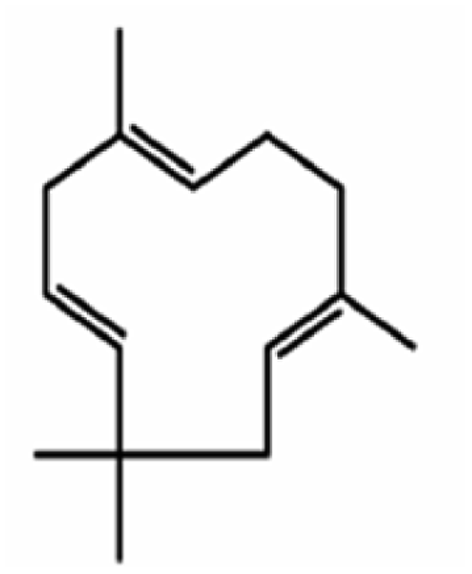Fig. 1 Structure of α-humulene (C₁₅H₂₄).

Methodology

Experimental setup

All experiments were carried out in the smog chamber of the Carnegie Mellon University (CMU) Center for Atmospheric Particle Studies (CAPS) (Fig. 2). The chamber is a 10 m³ Teflon reactor suspended in a temperature-controlled room and surrounded by UV lights. The chamber is flushed with purified air with the UV lights on for at least 8–10 hours prior to running an experiment. The air is purified passing through HEPA and activated carbon filters and also through silica gel to reduce the relative humidity to <10%. The NO_x levels in the chamber were always close to zero during these experiments. NO_x was measured used a Teledyne API, Model 200 A NO_x analyser which has a detection limit of 0.4 ppb.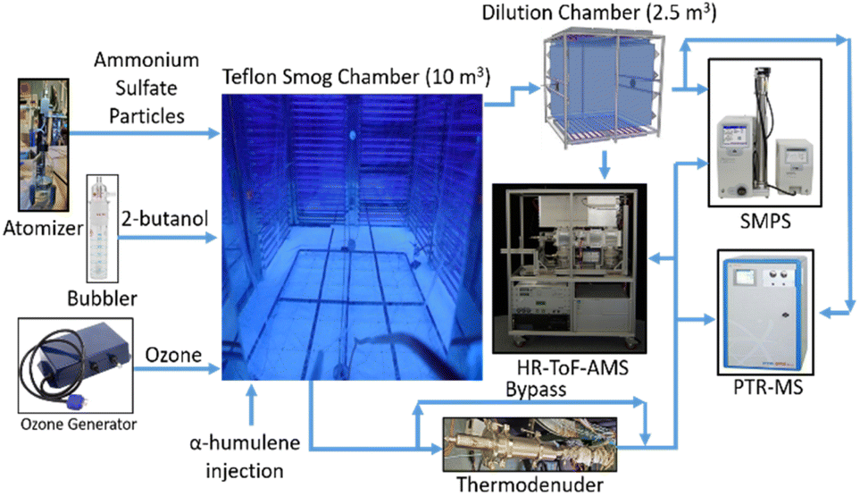

Fig. 2 Experimental set-up used in this study. The thermodenuder and dilution chamber were used in selected experiments to quantify the volatility distribution of the produced SOA.

After filling the reactor with clean air, a TSI atomizer (model 3076) was used to generate ammonium sulfate droplets. The droplets were then sent through a diffusion dryer, and the water evaporated resulting in dry ammonium sulfate particles. The particles were injected into the chamber to provide a pre-existing surface area for the SOA to condense on. The next 2 hours were used as a period for the measurement of the particle wall-loss rates to the walls of the chamber.

In the next stage a small amount of d₉-butanol was added into the chamber. The d₉-butanol was used as a tracer for the OH radical following the approach of Barmet et al.²³ The d₉-butanol concentration and the concentrations of other VOCs in the chamber were tracked by a proton-transfer reaction mass spectrometer (PTR-MS, Model QMG-422, Ionicon Analytic).

After the d₉-butanol concentration in the chamber had stabilized, an excess amount of ozone was generated using a corona discharge ozone generator (HTU-500, AZCO Industries LTD.) and transferred into the chamber. The ozone was allowed time to mix throughout the chamber until its concentration stabilized. The ozone concentration was measured using an ozone monitor (Teledyne, Model T400). After this point the chamber was ready for the injection of α-humulene.

Sesquiterpenes are “sticky” molecules, so they can easily be lost to the walls of tubing and of instruments.²⁴ Therefore, a heated septum injection system was used to ensure that practically all of the injected sesquiterpene is transferred into the chamber. A small volume of liquid α-humulene was measured and drawn into a syringe. Clean air was preheated and passed through the injection point for 10 min. The syringe was then inserted into the septum injection point, and the α-humulene was gradually injected over 2 min. This was defined as the starting point (time zero) of the experiment. To clear the septum of any residual α-humulene, clean air was passed through the septum for an additional hour. The experiments lasted for 4–6 hours. After the experiments ended, purified air was used to flush the chamber and the cleaning procedure was started. Eight experiments were performed in this study (Table 1), with the initial α-humulene concentration varying from 4 to 42 ppb.

Table 1 Experimental conditions

Exp	VOC (ppb)	O3 (ppb)	Seeds (μg m^−3)	SOA (μg m^−3)	SOA yield (%)
1	4	375	27	11	33
2	11	1100	35	62	70
3	42	465	0	155	55
4	11	310	30	48	52
5	11	275	80	38	41
6	11	330	140	55	60
7	5	345	26	12	28
8	12	290	72	63	64

---

A scanning mobility particle sizer (SMPS, TSI classifier model 3082, CPC model 3775, DMA model 3081) was used to measure the particle number and volume distributions and the corresponding concentrations. The mass concentrations, along with the chemical composition, of the particles were monitored using a high-resolution time-of-flight mass spectrometer (HR-ToF-AMS, Aerodyne Research, Inc.).

The thermodenuder (TD) described in An et al.²⁵ was used to measure the SOA volatility distribution. The SOA was sampled through either the TD or a bypass line (Fig. 2). This was done by switching the flow using two three-point valves. A dilution chamber (Teflon, 2.5 m³) was also used for the measurement of the volatility distribution using isothermal dilution. A metal bellows pump (Baldor, model MB-302) was used to transfer particles from the main chamber to the dilution chamber. The PTR-MS also sampled from the dilution chamber to determine the dilution ratio and the SMPS measured the particle size distribution in this reactor (Fig. 2). The combination of thermodenuder and isothermal dilution measurements provides a better constraint of the SOA volatility distribution.²⁶ Both the thermodenuder and isothermal dilution techniques provide driving forces that cause evaporation of the particles and in this way provide information about their volatility. The thermodenuder uses heating; therefore, the observed particle evaporation in this instrument depends both on the volatility of the particles at room temperature and on their enthalpy of vaporization. A major advantage of the technique is that it can observe the full evaporation of the particles.

Isothermal dilution uses dilution at room temperature to evaporate the particles. The observed evaporation depends only on the volatility at room temperature. However, because there are limits to how much the particles can be diluted this technique can usually observe only the partial evaporation of the particles (10–30% of their mass). Their combination has the advantages of both for the challenging estimation of several parameters (volatility distribution, enthalpy of vaporization, potential resistances to mass transfer) at the same. The measurements for the TD have been corrected using the temperature and size dependent particle loss corrections following the approach of Cain et al.²⁶

Data analysis

SQUIRREL 1.60O (SeQUential Igor data RetRiEvaL) and Pika 1.60O (peak integration by key analysis) were used for the HR-ToF-AMS data analysis. The AMS collection efficiency (CE) is the fraction of the particulate matter mass measured by the instrument. It is usually less than unity and is the product of three efficiencies that result from the difficulty of getting all the particles and their components through different parts of the AMS. An extended version of the Kostenidou et al.²⁷ algorithm based on the combination of the SMPS and AMS size distributions was used for the estimation of the AMS collection efficiency (CE) and the SOA density. The original version of the algorithm assumes that the same CE applies to all particles in the experiment, and therefore that the CE is size independent. However, this method was not appropriate for our experiments because two modes of particles existed: one due to nucleation and growth with particles only consisting of SOA and a second that contained ammonium sulfate coated with SOA. These two modes were fitted independently, and two CE values were determined, one for each mode. The organic-only mode had a much higher CE than the particles in the ammonium sulfate/organic mode. The CE for both modes was estimated as a function of time with an averaging period of one hour.

Size-dependent wall-loss corrections

One major challenge of smog chamber experiments is the loss of particles to the walls. These wall-losses decrease the measurable mass inside the chamber, and they can be characterized as a first-order process.²⁸ To characterize the wall-losses, experiments with inert non-volatile ammonium sulfate particles were performed. After the particles were injected, they were allowed to stay in the chamber undisturbed for about 2 hours. The SMPS measurements of the evolution of their size distribution were used then to estimate the size-dependent particle wall-loss rate constant using the approach presented by Nah et al.²⁹ The corresponding estimates of the size-dependent wall-loss rate constant are averaged during each experiment. These constants were determined before each experiment.

We tried to minimize the wall losses of the gas-phase products of α-humulene by using high concentrations of seeds. In this way, most of the produced material should condense on the pre-existing particles and should not be lost to the walls. No additional vapour loss corrections were used for these experiments. When there are no seed particles there is a period in which the concentration of the condensable organic compounds is above the saturation threshold but below the nucleation threshold. During this period there is rapid condensation to the walls of the chamber. Under certain conditions it is even possible for no SOA to be formed as the nucleation threshold may never be exceeded. The seed particles allow the SOA to start forming as soon as the system reaches saturation. The use of neutral non-volatile spherical seeds like ammonium sulfate is considered optimum. Organic seeds could complicate the situation by interacting with the SOA (e.g., forming a solution or multiple phases in the particles), could react with the various oxidants, etc.

Before the ozonolysis reaction begins (t = 0), the chamber only contains ammonium sulfate particles. After correcting for particle wall-loss, the volume concentration before the ozonolysis reaction was for all practical purposes stable. The increase in volume after the reaction begins is due to the formation of SOA. The wall-loss corrected SOA volume can be calculated as the difference between the wall-loss corrected total volume and the ammonium sulfate seed volume:

V^SOA(t) = V^tot(t) − V^seed (1)

The wall-loss corrected SOA volume is then converted to the wall-loss corrected SOA mass [M^SOA(t)] by multiplying with the organic aerosol density obtained from the Kostenidou et al.²⁷ algorithm. The above procedure was applied to the concentrations of both the dilution and main chamber.

SOA yield calculations

The SOA yield, Y_SOA, for each experiment was estimated based on:where C_SOA is the concentration of the produced SOA at the end of the experiment and C_sesq,Inj is the concentration of α-humulene injected. For these experiments, the yields were based on the SMPS data. Since it was not possible to measure accurately the total concentration of α-humulene injected due to its high reactivity and the limitation of the available PTR-MS to measure the concentrations of large organic molecules (with m/z higher than 200), it was assumed that all the injected α-humulene was injected into the chamber and reacted. The characteristic reaction times for the initial reaction between α-humulene and ozone in our experiments were less than 2 min for all cases.

Results

We first present and discuss the results of a typical experiment. In exp. 1, 4 ppb α-humulene reacted with 375 ppb O₃. A simple kinetic model of the three stages of ozonolysis of the α-humulene suggests that the reaction of the first double bond was quite fast and required less than 2 min in this experiment, while the reactions of the second double were completed after approximately 30 min. All three double bonds had reacted (95% completion) after approximately 5 h for.

The ammonium sulfate aerosol volume was reduced from 27 μm³ cm⁻³ to 19 μm³ cm⁻³ during the 2 h before the injection of the α-humulene (Fig. 3). The size-dependent wall-loss rate constant was approximately 0.11 h⁻¹ for particles with diameter higher than 250 nm and increased to 0.42 h⁻¹ for 50 nm particles and 0.57 h⁻¹ for 30 nm ones. After applying the size-resolved wall-loss rate constant the corrected ammonium sulfate volume remained constant at 27 μm³ cm⁻³ (mass concentration 46.9 μg m⁻³) for the seeds-only 2 hours period before the injection of the α-humulene (Fig. 3).

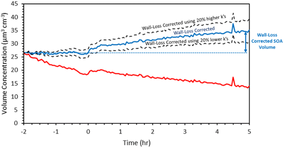Fig. 3 SMPS measured total volume concentration (red), wall-loss corrected concentration (blue), and uncertainty range for exp. 1.

In the 10 min period after the injection the particle volume increased by 2 μm³ cm⁻³. During this initial period ozone has completely reacted with the first double bond of α-humulene and the reaction of the second double bond is at the 50% level approximately. The SOA density calculated from the Kostenidou et al.²⁷ algorithm for this experiment was 1.3 g cm⁻³, therefore approximately 2.6 μg m⁻³ of SOA were produced during this initial stage of the experiment. The corresponding SOA yield in this first generation of reactions, assuming that the reacted α-humulene was equal to the injected amount was 7% (at SOA = 2.6 μg m⁻³). After this initial rapid SOA production, the wall-loss corrected SOA concentration continued to increase as the second and third double bonds were reacting.

After 5 h of reactions the estimated SOA concentration was 11 μg m⁻³ and the SOA yield increased to 33% (Fig. 4a). At this stage the SOA level was reaching asymptotically a plateau, including the uncertainty due to the wall loss corrections. To confirm that this later stage production of SOA is not an artifact of our wall-loss correction approach we estimated the corresponding uncertainty. In this experiment 70% of the particle mass (based on the SMPS measurements) was in diameter range above 150 nm. The wall loss-rate constant uncertainty for this size range was approximately 20%. Using this uncertainty, the final estimated SOA concentration ranged from 7.8 μg m⁻³ to 14.6 μg m⁻³ (Fig. 4a). So even if we consider the lower bound of the wall-loss corrected SOA there is production of additional SOA during the second and third generation of reactions of α-humulene of at least 6.8 μg m⁻³.

Fig. 4 (a) SMPS wall-loss corrected SOA mass concentration (blue) and corresponding uncertainty bounds for exp. 1 and (b) concentration of ozone during exp.1.

The different phases of the α-humulene ozonolysis can be seen in the behavior of the ozone concentration in this experiment (Fig. 4b). Ozone decayed rapidly during the first couple of minutes as it reacted mostly with the first double bond of the injected organic. The noisy behavior is due to the fact that the chamber was not perfectly mixed during these first few minutes. Then there is a second phase with slower ozone decay as it reacted mainly with the second double bond and finally a third phase with an even slower decay as the slower reactions with the third bond were still proceeding. One should note that there were also losses of ozone to the chamber walls during this period. The ozone levels decreased from 375 ppb to 340 ppb during this experiment.

α-Humulene SOA yields

The measured SOA final yields ranged from 30 to 70% for SOA concentrations between 10 and 100 μg m⁻³ (Fig. 5) suggesting that indeed α-humulene is a good SOA precursor.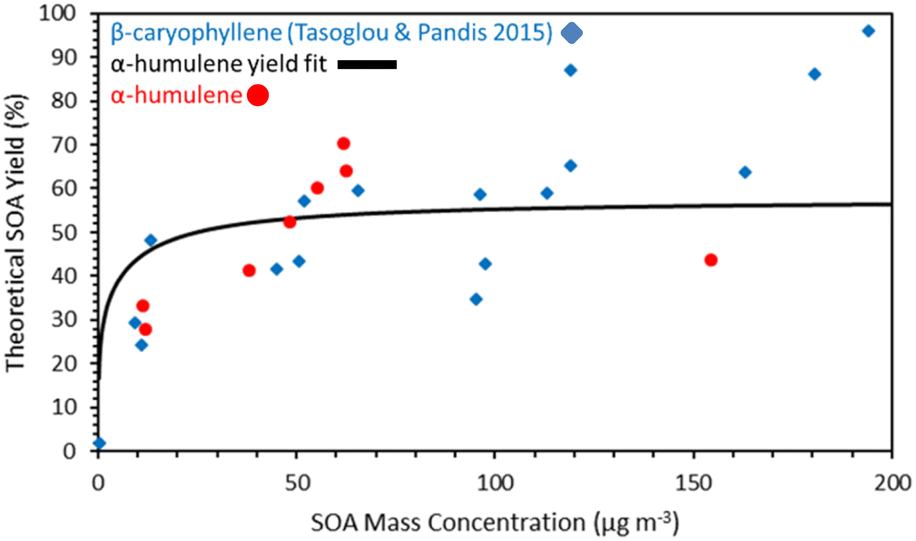

Fig. 5 Comparison of the α-humulene ozonolysis SOA yields measured in this work and the yield fit for those yields estimated by the Uruci et al.³¹ algorithm with the β-caryophyllene SOA yields ozonolysis of Tasoglou and Pandis.³⁰

The measured SOA yield was derived dividing the measured SOA concentration by the initial α-humulene concentration calculated based on the injected amount and the volume of the chamber. The different values for approximately the same loading indicate the variability of our results that are due to uncertainties in the reacted α-humulene, the corrections for losses and other experimental issues. While the results of the various experiments are in general consistent, the yield of experiment 3 is an outlier. For exp. 3, the SOA yield was 43% for an SOA concentration of 155 μg m⁻³. Based on the trend in the yields of the other experiments, it was expected that the yield for exp. 3 would be higher than 43%, especially because the initial concentration of α-humulene was much higher than the other experiments. The reason for this discrepancy could be because exp. 3 was the only experiment without any ammonium sulfate seeds. Therefore, the SOA mass lost on the walls would be greater compared to the other experiments.

The measured α-humulene SOA yields are quite similar to those of the β-caryophyllene ozonolysis determined in Tasoglou and Pandis³⁰ also shown in Fig. 6. For example, for SOA concentrations around 10 μg m⁻³ the α-humulene SOA yield was 28–33% and the β-caryophyllene yield was 24–30%. There is some evidence that for concentrations above 50 μg m⁻³ the α-humulene yields increased faster than those of β-caryophyllene, but these concentrations are quite high, and thus less relevant for the ambient atmosphere.

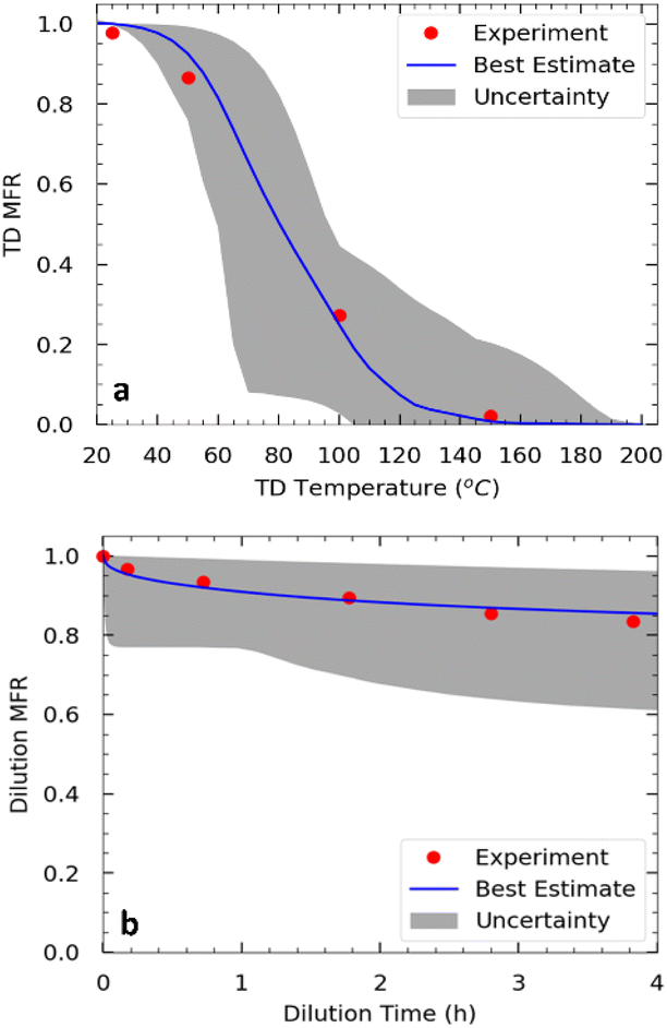Fig. 6 Measured (red symbols) and predicted (blue line): (a) thermogram and (b) areogram (dilution factor = 17.1) for the SOA from α-humulene ozonolysis for exp. 3.

These results suggest that the hypothesis of similar SOA yields of α-humulene and β-caryophyllene is valid and support the use of β-caryophyllene as a surrogate compound for all sesquiterpenes at least as a zeroth order approximation.

SOA volatility distribution

Approximately half of the SOA produced in exp. 3 evaporated at 80 °C (Fig. 6). Practically all the SOA evaporated at 140 °C after isothermal dilution by a factor of 17, approximately 15% of the SOA evaporated.

The SOA volatility distribution was estimated using the algorithm of Uruci et al.³¹ This algorithm combines yield, TD, and isothermal dilution measurements, to estimate the volatility distribution of the SOA, its vaporization enthalpy, the accommodation coefficient, and their uncertainties. This algorithm also provides an uncertainty range of the estimated yields at different temperatures and SOA levels. The estimated parameters are shown in Table 2 and the corresponding fits for the thermogram and areogram are shown in Fig. 6. Similar to how thermograms are plots of the particle mass fraction remaining (MFR) vs. the vaporization temperature of the TD, aerograms are plots of the particle MFR over time for the isothermal dilution experiments. Based on this estimated volatility distribution, about 37% of the SOA mass derived from low volatility organic compounds (LVOCs) while 63% was due to semivolatile organic compounds (SVOCs).

Table 2 Volatility distribution α-humulene SOA

		Stoichiometric coefficients (αi)
ΔHvap (kJ mol^−1)	log(αm)		10^−2	10^−1	10^0	10^1
115 ± 23	−2 ± 1		0.118 ± 0.083	0.094 ± 0.083	0.116 ± 0.096	0.247 ± 0.142

---

SOA AMS mass spectra

The SOA AMS mass spectra measured in the beginning and in the end of exp. 1 are shown in Fig. 7. They are characterized by a strong peak at m/z 43, and significant peaks at m/z 39, 41, 44, 53, 55, 64, 81 and 91.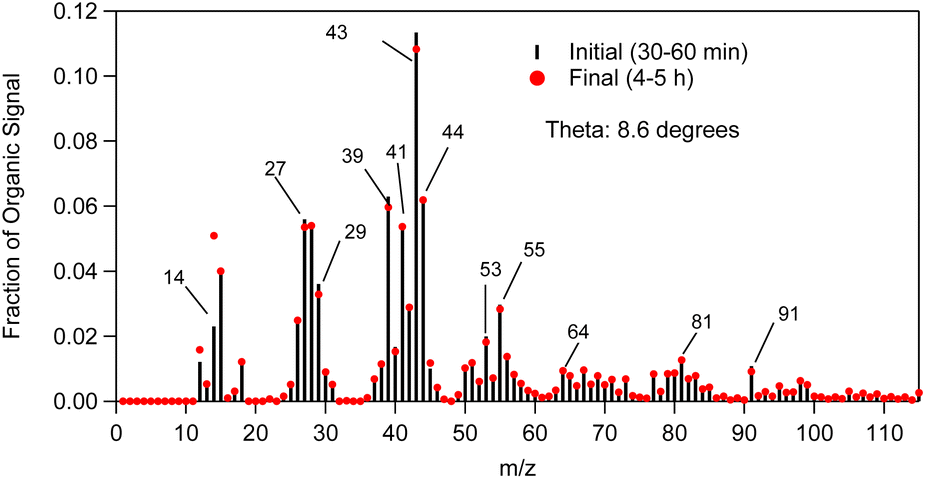

Fig. 7 α-Humulene SOA AMS mass spectra measured in the beginning (t = 30–60 min, black sticks) and at the end (t = 4–5 h, red dots) of exp. 1.

To qualitatively compare the SOA AMS spectra measured in the beginning and at the end of our experiments, the θ angle was calculated.³² The theta angle (θ) is a similarity metric of two AMS mass spectra. If both spectra are treated as vectors, theta is their angle. The cosine of the angle θ is equal to the correlation coefficient R. The SOA AMS spectrum was slowly evolving during the experiment and the angle between the initial spectrum and that at the end of the experiment was approximately 9°. A θ angle between two AMS spectra in the 0–5° range indicates an excellent match and the compared spectra should be considered identical for all practical purposes (R² ranging from 1 to 0.99). For a θ angle of 6–10° there is a good match (R² approximately 0.98–0.96), but there are some small differences. A θ of 11–15° shows that the spectra are quite similar, but they are not the same (R²: 0.95–0.92), while for a θ in the 16–30° range the spectra are originating from different sources, but there are some similarities (R²: 0.91–0.73). These results suggest that there were some modest differences in the composition of the SOA produced in the later stage of the α-humulene compared to the compounds produced in the initial stage.

Fig. 8 shows the AMS O : C ratio of the α-humulene ozonolysis SOA of exp. 1. After the first 15 min of the experiment, the O : C ratios were averaged every 15 min. The O : C of the SOA increased rapidly to about 0.25 and remained relatively constant for the remainder of the experiment. Part of this initial increase may be due to the small amounts of organic impurities in the ammonium sulfate particles, but part of it probably indicates that the initial products have a lower O : C than the rest. This is similar to the β-caryophyllene SOA O : C ratio of 0.31 ± 0.04 determined in Tasoglou & Pandis.³⁰

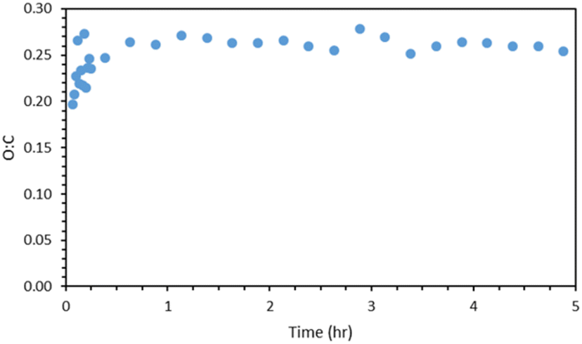Fig. 8 AMS O : C ratio for exp. 1, averaged every 15 min after t = 0.25 h.

The θ angle between the average AMS spectrum of the α-humulene ozonolysis SOA of this study and that of β-caryophyllene ozonolysis SOA of Tasoglou & Pandis³⁰ was 14° (Fig. 9). Similarities between these mass spectra are expected as both SOA derive from sesquiterpenes. Common dominant fragments across both spectra were at m/z's 39, 41, 43, 53, 55, 81 and 91. Some fragments that could be used to distinguish the spectra from each other include m/z's 64, 73 and 80 as these fragments showed more abundant signal for α-humulene SOA in comparison to β-caryophyllene SOA. On the other hand, m/z's 67 and 95 had higher contribution in the β-caryophyllene SOA mass spectrum.

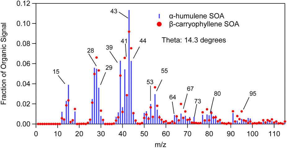Fig. 9 α-Humulene SOA mass spectrum measured in the beginning (t = 30–60 min, blue sticks) of exp. 1 compared to β-caryophyllene ozonolysis SOA mass spectrum (red dots) from Tasoglou and Pandis (2015).

Fig. 10 compares the mass spectrum of α-humulene ozonolysis SOA of this study to a typical α-pinene ozonolysis SOA mass spectrum. The θ angle calculated between these two mass spectra was 21°. The most distinct differences were at m/z's 43, 44, 56, 64, 67, 73, 80, 98 and 99. Fragments at m/z's 56 (C₃H₄O⁺), 64 (C₅H₄⁺) and 73 (C₃H₅O₂⁺ and C₄H₉O⁺) were higher in the α-humulene SOA spectrum. This was also the case for m/z's 98 (C₈H₂⁺, C₅H₆O₂⁺, C₆H₁₀O⁺) and 99 (C₅H₇O₂⁺) which had though lower intensity. The fragments at m/z's 64 and 73 could be used as chemical signatures for α-humulene SOA in order to potentially distinguish it from α-pinene SOA. Table 3 presents the angle theta and the coefficient of determination R² between the AMS mass spectra of α-humulene SOA and some biogenic SOA mass spectra in the literature.^{5,30,33,36–38} “Biogenic SOA” is a factor proposed by Kostenidou et al.³³ in their analysis of ambient OA measurements in Greece. According to these authors this corresponded to SOA produced as air masses were passing over forested areas before arriving to the sampling site. The lower angle theta, and thus higher similarity was observed for β-caryophyllene and limonene ozonolysis SOA (angle theta 14 and 17° respectively). The higher discrepancies were calculated for individual norpinic SOA components such as norpinic acid and MBTCA, which are considered as α- and β-pinene SOA tracers.

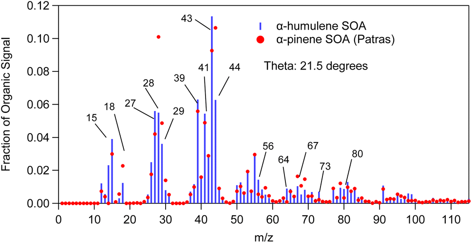Fig. 10 α-Humulene SOA mass spectrum measured in exp. 1 compared to α-pinene ozonolysis SOA mass spectrum (red dots).

Table 3 Comparison between α-humulene ozonolysis SOA and biogenic SOA mass spectra

	Theta angle (R^2)	Ref.
Biogenic SOA	31° (0.69)	Kostenidou et al.^33
Isoprene-SOA	30° (0.70)	Xu et al.^5
β-Caryophyllene + O3 SOA	14° (0.92)	Tasoglou and pandis^30
Limonene + O3 SOA	17° (0.89)	Kostenidou (unpublished data)^34
α-Pinene + O3 SOA	21° (0.84)	Kostenidou (unpublished data)^35
Norpinic acid	39° (0.51)	Kostenidou et al.^36
MBTCA	41° (0.49)	Kostenidou et al.^37

---

Conclusions

In this study, we examined the formation of SOA from the dark-ozonolysis of α-humulene. These experiments resulted in high SOA yields ranging from 30 to 70% for SOA concentrations in the range of 10 to 100 μg m⁻³. These yields are higher than those reported by Beck et al.¹⁶ who did not use seeds in their experiments. However, the measured SOA yields were similar those of the β-caryophyllene ozonolysis in Tasoglou & Pandis³⁰ for SOA concentrations less than 50 μg m⁻³. This result supports the use of β-caryophyllene as a surrogate compound for α-humulene, at least as a zeroth order approximation. Most of the SOA had effective volatility at 298 K equal or less than 1 μg m⁻³ and a significant fraction (mass yields around 20%) were low volatility organic compounds (LVOCs). The effective SOA vaporization enthalpy was 115 ± 23 kJ mol⁻¹. The α-humulene SOA appears to contain more LVOCs than that produced by the β-caryophyllene ozonolysis probably because it has an extra double bond. The α-humulene ozonolysis SOA density was 1.3 g cm⁻³ and its average O : C was 0.25 ± 0.02.

The α-humulene ozonolysis SOA mass spectrum was slowly evolving during experiments, and the angle of the corresponding vector with the initial spectrum at the end of the experiment was approximately 9°. This suggests modest differences, as far as the AMS is concerned, between the SOA compounds produced initially and the SOA compounds produced towards the end of the experiment. These changes probably will not be detectable under ambient conditions. The α-humulene SOA mass spectrum at the beginning of the SOA formation showed similarities with the β-caryophyllene ozonolysis SOA spectrum with an angle theta of 14°. However, it resembled less the α-pinene ozonolysis SOA spectrum. The main differences were due the m/z's 39, 41, 43, 44, 56, 64, 67, 73, 80, 98 and 99. Fragments at m/z's 64 and 73 were higher in the α-humulene SOA spectrum.

One of the issues raised by single precursor studies like the present one is the applicability of the results for the ambient atmosphere. Given the complexity of the chemical pathways leading to the SOA components and the uncertainty of the properties (e.g., saturation vapor pressures of these compounds) all current chemical transport models use some parameterization of SOA yields based on experiments with a single precursor. The models still account for other pollutants through the partitioning of the products to the organic particulate matter, the dependence of the yields on NO_x, the simulation of the coupled gas-phase chemistry of all organic compounds, the parameterizations of aging reactions, etc. The individual concentration, temperature and NO_x dependent yields serve as the first order approximation of these processes. They also serve as the baseline for the quantification of the importance of the interactions of the various precursors as they react together on their respective yields. The investigation of these interactions is quite time consuming because it involves experiments of combinations of precursors and comparisons of the SOA formed from the mixture with the sum of the individual yields. There is a number of recent efforts to study the SOA formation during the oxidation of mixtures of VOCs.^39–41 These studies do find changes in the composition of the SOA but the overall changes in the volatility distribution of the products and the total SOA yields appear to be modest. These studies of mixtures are valuable, but they still depend on the single precursor experiments for testing the yield additivity. So indeed, these VOCs never react on their own, but understanding the SOA formation in single precursor experiment remains a useful step in understanding eventually the importance of their interactions.

Conflicts of interest

There are no conflicts to declare.

Acknowledgements

This work was supported by the project FORCeS funded from the European Union's Horizon 2020 research and innovation programme under grant agreement No 821205. We also acknowledge support by the project by the project CHEVOPIN funded by the Hellenic Foundation for Research & Innovation (HFRI) under grant agreement no. 1819.

Notes and references

1. J. De Gouw and J. L. Jimenez, Organic aerosols in the Earth's atmosphere, Environ. Sci. Technol., 2009, 43, 7614–7618.
2. M. Hallquist, J. C. Wenger, U. Baltensperger, Y. Rudich, D. Simpson, M. Claeys, J. Dommen, N. M. Donahue, C. George, A. H. Goldstein, A. F. Hamilton, H. Herrmann, T. Hoffman, Y. Iinuma, M. Jang, M. E. Jenkin, J. L. Jimenez, A. Kiendler-Scharr, W. Maenhaut, G. McFiggans, Th. F. Mentel, A. Monod, A. S. H. Prévot, J. H. Seinfeld, J. D. Surratt, R. Szmigielski and J. Wildt, The formation, properties and impact of secondary organic aerosol: current and emerging issues, Atmos. Chem. Phys., 2009, 9, 5155–5236.
3. S. N. Pandis, K. Skyllakou, K. Florou, E. Kostenidou, C. Kaltsonoudis, E. Hasa and A. A. Presto, Urban particulate matter pollution: a tale of five cities, Faraday Discuss., 2016, 189, 277–290.
4. J. H. Seinfeld and S. N. Pandis, Atmospheric Chemistry and Physics: from Air Quality to Climate Change, John Wiley and Sons, New York, 3rd edn, 2016.
5. L. Xu, H. Guo, C. M. Boyd, M. Klein, A. Bougiatioti, K. M. Cerully, J. R. Hite, G. Isaacman-VanWertz, N. M. Kreisberg, C. Knote, K. Olson, A. Koss, A. H. Goldstein, S. V. Hering, J. De Gouw, K. Baumann, S. H. Lee, A. Nenes, R. J. Weber and N. L. Ng, Effects of anthropogenic emissions on aerosol formation from isoprene and monoterpenes in the southeastern United States, Proc. Natl. Acad. Sci. U. S. A., 2015, 112, 37–42.
6. H. Zhang, L. D. Yee, B. H. Lee, M. P. Curtis, D. R. Worton, G. Isaacman-VanWertz, J. H. Offenberg, M. Lewandowski, T. E. Kleindienst, M. R. Beaver, A. L. Holder, W. A. Lonneman, K. S. Docherty, M. Jaoui, H. O. T. Pye, W. Hu, D. A. Day, P. Campuzano-Jost, J. L. Jimenez, H. Guo, R. J. Weber, J. De Gouw, A. R. Koss, E. S. Edgerton, W. Brune, C. Mohr, F. D. Lopez-Hilfiker, A. Lutz, N. M. Kreisberg, S. R. Spielman, S. V. Hering, K. R. Wilson, J. A. Thornton and A. H. Goldstein, Monoterpenes are the largest source of summertime organic aerosol in the southeastern United States, Proc. Natl. Acad. Sci. U. S. A., 2018, 115, 2038–2043.
7. B. Friedman and D. K. Farmer, SOA and gas phase organic acid yields from the sequential photooxidation of seven monoterpenes, Atmos. Environ., 2018, 187, 335–345.
8. C. M. Salvador, C. C. K. Chou, T. T. Ho, C. Y. Tsai, T. M. Tsao, M. J. Tsai and T. C. Su, Contribution of terpenes to ozone formation and secondary organic aerosols in a subtropical forest impacted by urban pollution, Atmosphere, 2020, 11, 1232.
9. X. Wang, X. Guo, W. Dai, S. Liu, M. Shen, Y. Liu, Y. Zhang, Y. Cao, W. Qi, L. Li, J. Cao and J. Li, Diurnal variations of isoprene, monoterpenes, and toluene oxidation products in aerosols at a rural site of Guanzhong plain, northwest China, Atmosphere, 2022, 13, 634.
10. J. T. Knudsen, L. Tollsten and L. G. Bergstrom, Floral scents-a checklist of volatile compounds by head-space techniques, Phytochemistry, 1993, 33, 253–280.
11. D. Helmig, J. Ortega, A. Guenther, J. D. Herrick and C. Geron, Sesquiterpene emissions from loblolly pine and their potential contribution to biogenic aerosol formation in the Southeastern US, Atmos. Environ., 2006, 40, 4150–4157.
12. Q. Chen, Y. L. Li, K. A. McKinney, M. Kuwata and S. T. Martin, Particle mass yield from β-caryophyllene ozonolysis, Atmos. Chem. Phys., 2012, 12, 3165–3179.
13. S. Richters, H. Herrmann and T. Berndt, Different pathways of the formation of highly oxidized multifunctional organic compounds (HOMs) from the gas-phase ozonolysis of β-caryophyllene, Atmos. Chem. Phys., 2016, 16, 9831–9845.
14. M. Kanakidou, J. H. Seinfeld, S. N. Pandis, I. Barnes, F. J. Dentener, M. C. Facchini, R. Van Dingenen, B. Ervens, A. Nenes, C. J. Nielsen, E. Swietlicki, J. P. Putaud, Y. Balkanski, S. Fuzzi, J. Horth, G. K. Moortgat, R. Winterhalter, C. E. L. Myhre, K. Tsigaridis, E. Vignati, E. G. Stephanou and J. Wilson, Organic aerosol and global climate modelling: a review, Atmos. Chem. Phys., 2005, 5, 1053–1123.
15. M. A. H. Khan, M. E. Jenkin, A. Foulds, R. G. Derwent, C. J. Percival and D. E. Shallcross, A modeling study of secondary organic aerosol formation from sesquiterpenes using the STOCHEM global chemistry and transport model, J. Geophys. Res., 2017, 122, 4426–4439.
16. M. Beck, R. Winterhalter, F. Herrmann and G. K. Moortgat, The gas-phase ozonolysis of α-humulene, Phys. Chem. Chem. Phys., 2011, 13, 10970–11001.
17. M. Dekermenjian, D. T. Allen, R. Atkinson and J. Arey, FTIR analysis of aerosol formed in the ozone oxidation of sesquiterpenes, Aerosol Sci. Technol., 1999, 30, 349–363.
18. R. J. Griffin, D. R. Cocker III, R. C. Flagan and J. H. Seinfeld, Organic aerosol formation from the oxidation of biogenic hydrocarbons, J. Geophys. Res., 1999, 104, 3555–3567.
19. A. Lee, A. H. Goldstein, M. D. Keywood, S. Gao, V. Varutbangkul, R. Bahreini and J. H. Seinfeld, Gas-phase products and secondary aerosol yields from the ozonolysis of ten different terpenes, J. Geophys. Res., 2006, 111, 1–18.
20. M. Jaoui, T. E. Kleindienst, K. S. Docherty, M. Lewandowski and J. H. Offenberg, Secondary organic aerosol formation from the oxidation of a series of sesquiterpenes: alpha-cedrene, beta-caryophyllene, alpha-humulene and alpha-farnesene with O₃, OH and NO₃ radicals, Environ. Chem., 2013, 10, 178–193.
21. N. L. Ng, J. H. Kroll, M. D. Keywood, R. Bahreini, V. Varutbangkul, R. C. Flagan, J. H. Seinfeld, A. Lee and A. H. Goldstein, Contribution of first-versus second-generation products to secondary organic aerosols formed in the oxidation of biogenic hydrocarbons, Environ. Sci. Technol., 2006, 40, 2283–2297.
22. D. E. Romonosky, Y. Li, M. Shiraiwa, A. Laskin, J. Laskin and S. A. Nizkorodov, Aqueous photochemistry of secondary organic aerosol of alpha-pinene and alpha-humulene oxidized with ozone, hydroxyl radical, and nitrate radical, J. Phys. Chem., 2017, 121, 1298–1309.
23. P. Barmet, J. Dommen, P. F. DeCarlo, T. Tritscher, A. P. Praplan, S. M. Platt, A. S. H. Prévot, N. M. Donahue and U. Baltensperger, OH clock determination by proton transfer reaction mass spectrometry at an environmental chamber, Atmos. Meas. Tech., 2012, 5, 647–656.
24. N. C. Bouvier-Brown, A. H. Goldstein, J. B. Gilman, W. C. Kuster and J. A. De Gouw, In-situ ambient quantification of monoterpenes, sesquiterpenes and related oxygenated compounds during BEARPEX 2007: implications for gas-and particle-phase chemistry, Atmos. Chem. Phys., 2009, 9, 5505–5518.
25. W. J. An, R. K. Pathak, B. H. Lee and S. N. Pandis, Aerosol volatility measurement using an improved thermodenuder: application to secondary organic aerosol, J. Aerosol Sci., 2007, 38, 305–314.
26. K. P. Cain, E. Karnezi and S. N. Pandis, Challenges in determining atmospheric organic aerosol volatility distributions using thermal evaporation techniques, Aerosol Sci. Technol., 2020, 54, 941–957.
27. E. Kostenidou, R. K. Pathak and S. N. Pandis, An algorithm for the calculation of secondary organic aerosol density combining AMS and SMPS data, Aerosol Sci. Technol., 2007, 41, 1002–1010.
28. N. Wang, S. Jorga, J. Pierce, N. Donahue and S. Pandis, Particle wall-loss correction methods in smog chamber experiments, Atmos. Meas. Tech., 2018, 11, 6577–6588.
29. T. Nah, R. C. McVay, J. R. Pierce, J. H. Seinfeld and N. L. Ng, Constraining uncertainties in particle-wall deposition correction during SOA formation in chamber experiments, Atmos. Chem. Phys., 2017, 17, 2297–2310.
30. A. Tasoglou and S. N. Pandis, Formation and chemical aging of secondary organic aerosol during the β-caryophyllene oxidation, Atmos. Chem. Phys., 2015, 15, 6035–6046.
31. P. Uruci, D. Sippial, A. D. Drosatou and S. N. Pandis, Estimation of secondary organic aerosol formation parameters for the Volatility Basis Set combining thermodenuder, isothermal dilution and yield measurements, Atmos. Meas. Tech. Discuss., 2023 DOI:10.5194/amt-2022-320 , in review.
32. E. Kostenidou, B. H. Lee, G. J. Engelhart, J. R. Pierce and S. N. Pandis, Mass spectra deconvolution of low, medium, and high volatility biogenic secondary organic aerosol, Environ. Sci. Technol., 2009, 43, 4884–4889.
33. E. Kostenidou, K. Florou, C. Kaltsonoudis, M. Tsiflikiotou, S. Vratolis, K. Eleftheriadis and S. N. Pandis, Sources and chemical characterization of organic aerosol during the summer in the eastern Mediterranean, Atmos. Chem. Phys., 2015, 15, 11355–11371.
34. E. Kostenidou, Unpublished work.
35. E. Kostenidou, Unpublished work.
36. E. Kostenidou, S. Jorga, J. K. Kodros, K. Florou, A. Kołodziejczyk, R. Szmigielski and S. N. Pandis, Properties and atmospheric oxidation of norpinic acid aerosol, Atmosphere, 2022, 13, 1481.
37. E. Kostenidou, E. Karnezi, A. Kołodziejczyk, R. Szmigielski and S. N. Pandis, Physical and chemical properties of 3-methyl-1,2,3-butanetricarboxylic acid (MBTCA) aerosol, Environ. Sci. Technol., 2018, 52, 1150–1155.
38. N. Wang, E. Kostenidou, N. M. Donahue and S. N. Pandis, Multi-generation chemical aging of α-pinene ozonolysis products by reactions with OH, Atmos. Chem. Phys., 2018, 18, 3589–3601.
39. G. McFiggans, T. F. Mentel, J. Wildt, I. Pullinen, S. Kang, E. Kleist, S. Schmitt, M. Springer, R. Tillmann, C. Wu, D. Zhao, M. Hallquist, C. Faxon, M. Le Breton, Å. M. Hallquist, D. Simpson, R. Bergström, M. E. Jenkin, M. Ehn, J. A. Thornton, M. R. Alfarra, T. J. Bannan, C. J. Percival, M. Priestley, D. Topping and A. Kiendler-Scharr, Secondary organic aerosol reduced by mixture of atmospheric vapours, Nature, 2019, 565, 587–593.
40. A. Voliotis, Y. Wang, Y. Shao, M. Du, T. J. Bannan, C. J. Percival, S. N. Pandis, M. R. Alfarra and G. McFiggans, Exploring the composition and volatility of secondary organic aerosols in mixed anthropogenic and biogenic precursor systems, Atmos. Chem. Phys., 2021, 21, 14251–14273.
41. A. Voliotis, M. Du, Y. Wang, Y. Shao, T. J. Bannan, M. Flynn, S. N. Pandis, C. J. Percival, M. R. Alfarra and G. McFiggans, The influence of the addition of isoprene on the volatility of particles formed from the photo-oxidation of anthropogenic–biogenic mixtures, Atmos. Chem. Phys., 2022, 22, 13677–13693.

---