 Open Access Article
Creative Commons Attribution 3.0 Unported Licence
Highly transferable atomistic machine-learning potentials from curated and compact datasets across the periodic table†
Christopher M.
Andolina
 a and
Wissam A.
Saidi
 *ab
*ab
aDepartment of Mechanical Engineering and Materials Science, University of Pittsburgh, Pittsburgh, PA 15261, USA. E-mail: alsaidi@pitt.edu
bNational Energy Technology Laboratory, United States Department of Energy, Pittsburgh, PA 15236, USA
First published on 3rd July 2023
Abstract
Machine learning atomistic potentials trained using density functional theory (DFT) datasets allow for the modeling of complex material properties with near-DFT accuracy while imposing a fraction of its computational cost. The curation of the DFT datasets can be extensive in size and time-consuming to train and refine. In this study, we focus on addressing these barriers by developing minimalistic and flexible datasets for many elements in the periodic table regardless of their mass, electronic configuration, and ground state lattice. These DFT datasets have, on average, ∼4000 different structures and 27 atoms per structure, which we found sufficient to maintain the predictive accuracy of DFT properties and notably with high transferability. We envision these highly curated training sets as starting points for the community to expand, modify, or use with other machine learning atomistic potential models, whatever may suit individual needs, further accelerating the utilization of machine learning as a tool for material design and discovery.
1. Introduction
Numerous studies on code the development, training, validation, and transferability of machine learning atomistic potentials (MLPs) have recently been reported, highlighting notable and significant advances in materials modeling.1–4 Many of these studies underscore that MLPs have high fidelity in simulating various properties and are significantly less computationally demanding than density functional theory (DFT) calculations.4 Therefore, MLPs can readily be used to model known materials at large sizes (a recent study claiming ten billion atoms5) and long timescales and to discover the applications of interest,6 further accelerating the computational modeling of materials.7 Recent refinements of machine learning (ML) approaches8,9 and training methodologies7,10 have further improved the accuracy, precision, and utility of these atomistic potentials and their use for various material applications.11 Computational material science has seized the development of these ML advances for chemical modeling applications12 and applied them to describe complex dynamic systems, including single elementals,13 bimetallic systems,14–16 supported metal nanoclusters,17 hybrid perovskites,18 and metal oxides.19 Although MLPs, in general, are less time-consuming to train/refine and more robust at describing systems outside of their training datasets (transferability)20–23 compared to classical atomistic potentials (e.g., embedded atom model potentials), the training workflow and database composition are areas that could benefit from further optimization, as noted in current reviews in literature.24,25We aim to further advance MLP development by providing a clear and systematic approach to curating minimalistic DFT datasets that can be applied to almost any element in the periodic table (Fig. 1). Creating databases to train ML potentials is a challenging endeavor regardless of the ultimate application of the atomistic potential.26 This study focuses on using deep neural network models to develop atomistic potentials. Although we specifically examine the predictive accuracy of the deep neural network potentials (DNP) with these DFT datasets, we expect other MLP models to have a similar accuracy based on prior investigations.27 We note there are few examples of these highly applicable methodologies for multiple (over 23) elements,28 which are distinct from this approach and rely on an automated workflow (DP-GEN).29
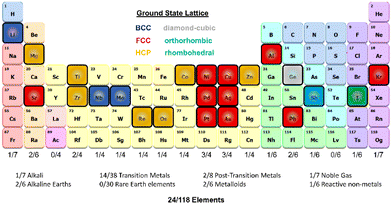 | ||
| Fig. 1 Schematic of the period table visualizing the elements selected for this work and highlighting the ground state lattice configurations. | ||
We demonstrate our approach by sampling elements with distinct masses, electron configurations, and ground-state crystal phases (excluding rare earth elements). Our method for developing single-element datasets depends on the curated Material Project database (MPDB)30 and the NOMAD repository and archive,31 and a DeePMD-kit neural network approach.32 We refine our DNP models using adaptive learning. We apply an ensemble approach to compare single-element inter-DNP deviations of randomly seeded models and select configurations with more significant force deviations for further training. The final single-element potentials were trained for up to three iterations, containing less than 3857 ± 1032 with an overall average of 27 ± 12 atoms per structure (see Table S1 for more details†). These DNPs can accurately predict several properties of five low-energy lattice configurations for each element. As shown below, the resulting potentials have good transferability to atomic environments not explicitly included in the training database (e.g., other lattice configurations, vacancies, surfaces, and the thermal stability of the solid phase).
2. Computational methods
2.1 Curation of the DFT dataset for DNP training
Initial DFT parent structures comprise five of the lowest energy lattice structures deposited in MPDB33 (e.g., face-center-cubic (fcc), body-center-cubic (bcc), hexagonal, hexagonal close-pack (hcp), rhombohedral, orthogonal, tetragonal, trigonal, simple cubic, and/or diamond cubic). If five structures were not located in the MPDB for a select element, additional lattice crystal systems were obtained from the NOMAD Repository and Archive31 or generated34 and optimized using DFT (VASP)35–37 before training. The specific lattices used for training vary from element to element; the ESI† provides a complete list of phases (Table S2†). Generally, for the ground state configuration, single-point defect structures (vacancy Table S4† or interstitial Table S5†) were generated from a DFT-optimized 2 × 2 × 2 supercell of the conventional lattice structure. Additionally, each dataset contained a set of deformed lattices in twelve directions, typically employed to calculate elastic constants from finite differences. For each parent structure (point defect type and each of the 12 deformed lattices), 20 configurations were generated from a molecular dynamics (MD) trajectory with constant volume and temperature (NVT) at two temperatures (Tm and 0.25 Tm) for the elements with melting temperatures Tm at <2000 K, and three temperatures (Tm, 0.6 Tm, and 0.25 Tm) for selected elements with Tm > 2000 K.The VASP calculations were performed using the Perdew–Burke–Ernzerhof (PBE) exchange–correlation functional with projector-augmented wave pseudopotentials,35–37 which correspond to those used by the corresponding elements listed in the MPDB.33,38 We selected a plane-wave cut-off of 400 eV that was used consistently across all materials. We used a tight break condition of 10−8 eV free energy change between steps in the electronic relaxation loop. Moreover, we applied Methfessel-Paxton39 smearing of 2nd-order with 0.15 eV, broadening to sample the Brillouin zone. We used a k-spacing value of 0.24 Å−1 for all calculations, which we previously showed to be sufficient for training purposes; the DNPs generated using the DFT training database were found to be less sensitive to errors from under-sampling the Brillouin zone than the standard DFT calculations.13
2.2 Description of the DNP training procedure
Machine learning potentials were trained using the DeePMD-kit (v2.1.2)40 within the DeepPot-SE41 approach. The DeePMD-kit utilizes neural networks to interpolate the relationship between atomic coordinates (model input samples) and energies, forces, and virials (model output labels) in the DFT training data. We used a consistent training protocol with identical hyperparameters for each DNP, including randomly initialized weights in the neural networks. The complete set of hyperparameters used for training is provided in a DeePMD-kit input file in the ESI.†Three DNPs with initial randomized weights were generated at each step of the iterative training process. LAMMPS was utilized to calculate various properties (vide infra) for each element. The averages and standard deviations of the DNP-calculated properties were examined and compared to the VASP reference properties with the same initial structures to determine the overall accuracy and precision of the potential. At least two training iterations (iterations 0 and 1) were performed for every element to hone the DNP accuracy.
2.3 DFT reference values
DFT material property references were calculated for the five lattices used as training data sets using VASP parameters similar to the training dataset. For basic lattice properties, such as lattice constants, unit cell volume per atom, and cohesive energy (Ecoh), we used a conventional primitive unit cell (1 × 1 × 1) and previously reported methodologies.16 We used a 2 × 2 × 2 supercell for single atom vacancies and interstitial structures.Elastic constant calculations were made using VASP with the same convergence thresholds, 2 × 2 × 2 supercell (if the conventional cell contained less than or equal to four atoms), IBRION value of six, and NFREE value of two. All other parameters were the same for the VASP static property calculations, including an energy cut-off of 400 eV. We used a POTMIN value of 0.01 Å for the atomic displacements. Our values generally agree with the elastic constant reported in the MPDB42 (Table S5†).
2.4 LAMMPS calculations
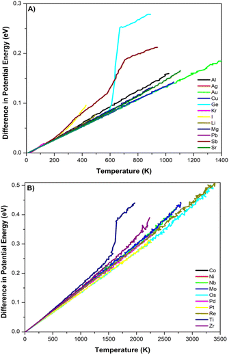
We have detailed descriptions of our process for calculating material properties using LAMMPS and the DNPs reported elsewhere in the literature.13–16 We used convergence criteria based on 1 × 10⁻¹⁰ eV for energy and forces between minimization steps. A 4 × 4 × 4 supercell was used for elastic calculations with a 0.005–0.01 Å displacement.Continuous heating curves for validation are obtained from molecular dynamic simulations employed within an NVT ensemble with one femtosecond timestep. The temperature was controlled using a Berendsen thermostat applied every 100 steps. The temperature was ramped (1 K per femtosecond) from 0 K to approximately 100 K above the experimental melting temperatures, starting with a ground-state lattice supercell relaxed at 0 (bar) pressure. We used 10 × 10 × 10 supercells for each element's identified ground-state lattice structure. We utilized a compressed version of the DNP for these MD heating simulations, which improved the speed of the simulation with a negligible impact on the accuracy of this calculation.
2.5 Validation check on non-trained structures
We assess the transferability of DNPs for each element on structures not explicitly included in the training. Some of the structures were gathered from the MPDB while some were generated43 by our group. We compared the DNP calculated and averaged cohesive energy (Ecoh), per atom volume, and elastic constants to the DFT reference values (Tables S8–S10†).2.6 Surface energy calculations
We utilized the LAVA code44 to calculate low-energy non-reconstructed Miller index surfaces (100), (110), and (111) (fcc, bcc, and diamond cubic phases and (0001), (10![[1 with combining macron]](https://www.rsc.org/images/entities/char_0031_0304.gif) 0) and (11
0) and (11![[2 with combining macron]](https://www.rsc.org/images/entities/char_0032_0304.gif) 0) for the hcp phase) surface energies using the LAMMPS wrapper with the DNPs. The average surface energies were determined from the three randomly seeded DNPs and compared to the corresponding DFT (VASP) calculated reference values from the MPDB.45
0) for the hcp phase) surface energies using the LAMMPS wrapper with the DNPs. The average surface energies were determined from the three randomly seeded DNPs and compared to the corresponding DFT (VASP) calculated reference values from the MPDB.45
3. Results and discussion
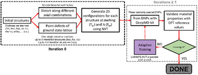
We developed a simplistic approach for generating and refining the DFT training dataset for 23 elements (Ag, Al, Au, Co, Cu, Ge, I, Li, Kr, Nb, Ni, Mg, Mo, Os, Pb, Pd, Pt, Re, Sb, Sr, Ti, Zn, and Zr) across the periodic table (Fig. 1) to develop robust DNPs that describe the base material properties for many temperatures, various phases, and selected point defects. The elements chosen in this study represent a wide range of melting temperatures (e.g., Kr and Os), atomic masses (e.g., Li and Pb), electron configurations, elemental groups, and ground state phases (11× fcc, 6× hcp, 2× bcc, 1× diamond cubic, 1× tetragonal, 2× orthorhombic). Applying these simplified and compact DFT training set criteria to a diverse selection of elements strongly suggests that this general approach applies to most elements on the periodic table for dataset creation, modeling, and refinement for DNPs, at least for single-element systems. We did not investigate the impact of tailoring the model's hyperparameters to each element of the training dataset, which may improve accuracy and performance; instead, we chose to use a “universal” set of parameters for all elements. Our dataset curation focused on achieving good accuracy of lattice constants, cohesive energies, single vacancy defects, interstitial atoms, elastic constants, and thermal stability of the solid phase between 0 K and the melting temperature.To generate 12 distortions of the lattice in the elastic limit for each lattice of the metal systems, we tested various thresholds from 0.01 to 0.05 Å. We found that the distortion of the lattice by 0.03 Å yielded DNPs that produced the most accurate results overall, with the smallest number of configurations. We ran NVT at the previously defined temperature(s) for each distorted structure to generate 20 configurations. Additionally, we included single vacancy structures for each phase and various self-interstitials (see below) for only the lowest energy phase of each element. In addition to the initial training set, we note that at most, two additional adaptive learning training iterations were required to produce elastic properties that converged with our calculated DFT reference values. The general workflow is depicted in Fig. 2.
As an additional quality check on the precision of the DNPs, while the training improves from iteration to iteration, the standard deviation between the three randomly seeded potentials decreases. We believe this ensemble approach to DNP validation is an important metric to highlight, as we envision these DFT datasets as a minimalistic “core” dataset that can be added to or combined for tailored applications by the community. Reporting the average value and the standard deviation of the values from the three DNPs allows others to assess the precision of the potential and determine whether these values are acceptable for their desired application or if more training is required. Overall, the maximum number of configurations used for training was less than 6100, with no more than 231![[thin space (1/6-em)]](https://www.rsc.org/images/entities/char_2009.gif) 000 total atoms per element (Table S1†).
000 total atoms per element (Table S1†).
3.1 Basic material properties and phases
We found excellent agreement between the predicted DNP and the DFT reference values for lattice constants and cohesive energies (Fig. 3, Tables S2 and S3†), exemplified by the proximity to the parity line and relatively small standard deviations, as shown in Fig. 2. The percent deviation from the DFT reference values is <12% (excluding Kr with cohesive energies (Ecoh) < 0.1 eV) per atom volume and <11% for Ecoh. The errors reported in the figures and ESI tables† are the standard deviation of the averaged material property from the three randomly seeded DNP potentials. Notably, we did not include any of these structures in the training data sets; only distorted or defected lattices at temperatures above 0 K were included, yet the prediction of the DNPs is accurate compared to DFT reference values reflecting its transferability.3.2 Point defects: vacancies and interstitials
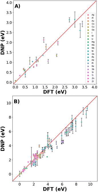
Real-world materials are not pristine and contain defects, such as vacancies and interstitials. Therefore, these common point defects were included in the training data sets for each element to improve the basic DNP applicability to real-world materials modeling (Fig. 4 and 6). We compare structures included and excluded in training for single vacancy defect energies (Fig. 4A and Table S4†). The vacancy energies can be relatively small (less than 1 eV), so some structure standard deviations appear more pronounced. Generally, we observe good agreement for most vacancy energies. However, we do not achieve the same accuracy for the energies of the non-defected ground state lattices exemplified in Fig. 3.For the self-interstitial facilities, we examine a large variety of tetrahedral (Td), octahedral (Oh), dumbbell (db), and crowdion for the lowest energy/ground state phase for each element provided the phase was bcc,46 fcc,16 diamond cubic,47 or hcp48 (Fig. 4B and Table S5†). We observe good agreement between the average DNP value and the calculated DFT value; however, we note that few interstitials exhibit significant standard deviations of the mean. Upon closer scrutiny, the corresponding interstitials were deemed unstable, as the initial and final structures exhibited an unusual change in the cell volume in the DFT reference calculations; therefore, they were omitted from the validation (Fig. 4 and Table S5†).
3.3 Elastic constants
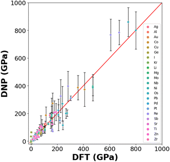
Generating DNPs that accurately predict elastic constants for multiple lattice phases per element is challenging, given that this relies on finite differences. This has not been frequently reported in the literature.19,49Fig. 5 compares the DNP and DFT calculation results for unique elastic constants (C11, C12, C13, C22, C33, C44, C55, and C66) for each element's ground state phase (Table S6†). DFT calculations of elastic constants can be highly sensitive to cut-off energies, k-grid spacings, and supercell size.13 We observe a more significant standard deviation for the elements with heavier nuclei and unfilled electron shells (e.g., Os and Re). Therefore, the observed standard deviations scale with the magnitude of the average value of the elastic constant.Here, we examine transferability by testing a limited number of phases (either from the MPDB or generated) per element and comparing them to DFT reference values.
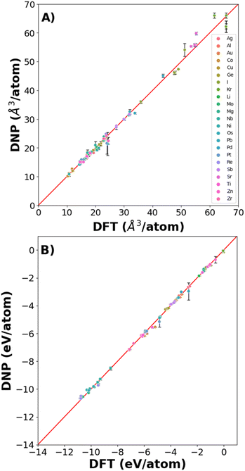
Fig. 6 shows that the potentials predict the per atom volume (Fig. 6A) and Ecoh (Fig. 6B) well, with only a small number of structures where Ecoh and per atom volumes were poorly predicted (Fig. 6 and Table S9†). However, the % average vacancy energy error (and standard deviation) in the single atom vacancy is more significant than we observed for the trained structures (Tables S4 and S10†), highlighting the boundaries of DNP transferability.
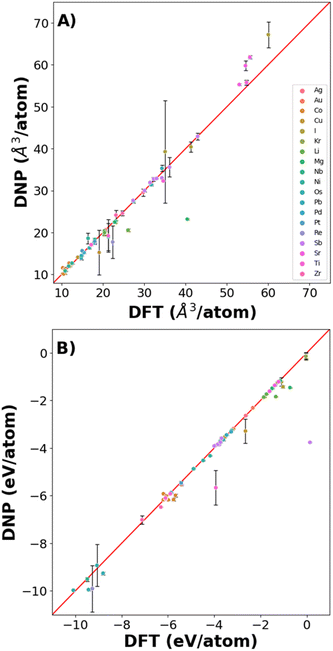 | ||
| Fig. 6 DNP predictive accuracy for phases not included in the training dataset for (A) volume/atom and (B) cohesive energy. | ||
Additionally, comparing the elastic constant for non-ground state phases demonstrates agreement with DFT reference values (Table S8†). Although the agreement is less than desirable for some of these lattices, additional training is necessary to describe the untrained vacancies and non-refined elastic constant predictions. However, the overall transferability of these simple phases and point defects is remarkable. Further, these DNPs can be extended to other properties.
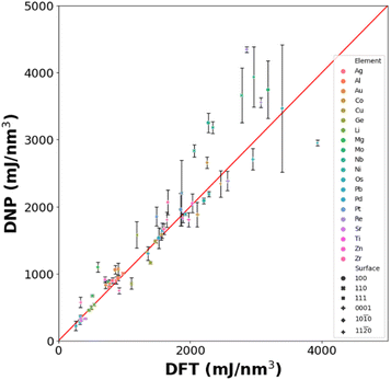
![[1 with combining macron]](https://www.rsc.org/images/entities/char_0031_0304.gif) 0), and (11
0), and (11![[2 with combining macron]](https://www.rsc.org/images/entities/char_0032_0304.gif) 0)) (Table S11†). Although further training is required to improve the accuracy of the surface energy predictions, the transferability of these DNPs is surprising, as we have not introduced any aperiodic structures resembling a surface in the training set.
0)) (Table S11†). Although further training is required to improve the accuracy of the surface energy predictions, the transferability of these DNPs is surprising, as we have not introduced any aperiodic structures resembling a surface in the training set.
4. Conclusions
We have described a general curation methodology by constructing relatively small sets of DFT configurations (<6000) for training single-element atomistic potentials using the DeePMD-kit with a DeepPot-SE approach. Our dataset curation recipe is effective for obtaining a diverse sampling of elements across the periodic table, describing various benchmark material properties with reasonable fidelity to DFT reference values. Additionally, we estimate the DNP's predictive accuracy range from the three randomized seeded versions to give a baseline range of values before the training sets are modified. Lastly, we found that these compact training sets, along with the DNP training approach, produced highly robust and transferrable potentials that could predict many properties that were not explicitly included in the training data. Ultimately, this study will allow users to augment and build upon these small datasets and/or curation methodologies for their unique scientific queries.Lastly, we note the various limitations and future extensions of and to this work that would benefit the community. Using these hand-curated systematic training datasets, we focused only on the DeepPot-SE approach and did not assess other MLP models. Such a comparative investigation of MLPs, similar to that of Zuo et al.27 or Morrow et al.,53 would be helpful to the community in assessing the fidelity of the dataset and model combination. We hope this study, particularly the developed and shared datasets, will motivate such extensive comparative studies. Additionally, informative metrics describing the DFT training dataset parameters, such as structural, energies, and forces landscapes, would be beneficial for evaluating and comparing training datasets regardless of the MLP model employed. We deem that these future works will be highly informative for all atomistic potential development and benchmarking going forward.
Data availability
(1) Data used to generate the main text figures are found in the ESI.†(2) Due to the large DFT training data file sizes, we have generated Github repository for these resources, which can be located by navigating to this link (https://github.com/saidigroup/23-Single-Element-DNPs). In addition, example validation scripts for both LAMMPs and VASP are archived, as well as the final iterations for all three randomly seeded DNPs for each of the 23 elements discussed in this study.
Author contributions
Christopher M. Andolina: conceptualization, data curation, formal analysis, investigation, methodology, resources, software, validation, visualization, writing – original draft. Wissam A. Saidi: conceptualization, formal analysis, funding acquisition, investigation, methodology, project administration, resources, software, supervision, writing – review & editing. Both authors discussed the results and reviewed the manuscript.Conflicts of interest
There are no conflicts to declare.Acknowledgements
We are grateful to the U.S. National Science Foundation (Award No. CSSI-2003808). We acknowledge R. Saidi for helping with Fig. 1. Computational support was provided in part by the University of Pittsburgh Center for Research Computing through the resources provided on the H2P cluster, which is supported by NSF (Award No. OAC-2117681).Notes and references
- J. Behler and G. Csányi, Eur. Phys. J. B, 2021, 94, 142, DOI:10.1140/epjb/s10051-021-00156-1.
- A. M. Miksch, T. Morawietz, J. Kästner, A. Urban and N. Artrith, Mach. Learn.: Sci. Technol., 2021, 2, 031001, DOI:10.1088/2632-2153/abfd96.
- J. Behler, J. Chem. Phys., 2016, 145, 170901, DOI:10.1063/1.4966192.
- Y. Mishin, Acta Mater., 2021, 214, 116980, DOI:10.1016/j.actamat.2021.116980.
- Z. Guo, D. Lu, Y. Yan, S. Hu, R. Liu, G. Tan, N. Sun, W. Jiang, L. Liu and Y. Chen, 27th PPoPP, 2022, pp. 205–218, DOI:10.1145/3503221.3508425.
- J. F. Rodrigues Jr, L. Florea, M. C. F. de Oliveira, D. Diamond and O. N. Oliveira Jr, Discov. Mater., 2021, 1, 12, DOI:10.1007/s43939-021-00012-0.
- J. Westermayr, S. Chaudhuri, A. Jeindl, O. T. Hofmann and R. J. Maurer, Digit. Discov., 2022, 1, 463–475, 10.1039/d2dd00016d.
- M. Haghighatlari, J. Li, X. Guan, O. Zhang, A. Das, C. J. Stein, F. Heidar-Zadeh, M. Liu, M. Head-Gordon, L. Bertels, H. Hao, I. Leven and T. Head-Gordon, Digit. Discov., 2022, 1, 333–343, 10.1039/d2dd00008c.
- V. Zaverkin, D. Holzmüller, I. Steinwart and J. Kästner, Digit. Disc., 2022, 1, 605–620, 10.1039/d2dd00034b.
- M. J. Burn and P. L. A. Popelier, Digit. Disc., 2023, 2, 152–164, 10.1039/d2dd00082b.
- L. Ward and C. Wolverton, Curr. Opin. Solid State Mater. Sci., 2017, 21, 167–176, DOI:10.1016/j.cossms.2016.07.002.
- S. Käser, L. I. Vazquez-Salazar, M. Meuwly and K. Töpfer, Digit. Disc., 2023, 2, 28–58, 10.1039/d2dd00102k.
- D. Bayerl, C. M. Andolina, S. Dwaraknath and W. A. Saidi, Digit. Disc., 2022, 1, 61–69, 10.1039/d1dd00005e.
- C. M. Andolina, J. G. Wright, N. Das and W. A. Saidi, Phys. Rev. Mater., 2021, 5, 083804, DOI:10.1103/PhysRevMaterials.5.083804.
- C. M. Andolina, M. Bon, D. Passerone and W. A. Saidi, J. Phys. Chem. C, 2021, 125, 17438–17447, DOI:10.1021/acs.jpcc.1c04403.
- C. M. Andolina, P. Williamson and W. A. Saidi, J. Chem. Phys., 2020, 152, 154701, DOI:10.1063/5.0005347.
- W. Chu, W. A. Saidi and O. V. Prezhdo, ACS Nano, 2020, 14, 10608–10615, DOI:10.1021/acsnano.0c04736.
- B. Wang, W. Chu, Y. Wu, D. Casanova, W. A. Saidi and O. V. Prezhdo, J. Phys. Chem. Lett., 2022, 13, 5946–5952, DOI:10.1021/acs.jpclett.2c01452.
- P. Wisesa, C. M. Andolina and W. A. Saidi, J. Phys. Chem. Lett., 2023, 14, 468–475, DOI:10.1021/acs.jpclett.2c03445.
- K. Lee, D. Yoo, W. Jeong and S. Han, Comput. Phys. Commun., 2019, 242, 95–103, DOI:10.1016/j.cpc.2019.04.014.
- G. Sivaraman, L. Gallington, A. N. Krishnamoorthy, M. Stan, G. Csányi, Á. Vázquez-Mayagoitia and C. J. Benmore, Phys. Rev. Lett., 2021, 126, 156002, DOI:10.1103/PhysRevLett.126.156002.
- A. V. Shapeev, Multiscale Model. Simul., 2016, 14, 1153–1173, DOI:10.1137/15m1054183.
- A. P. Bartók, M. C. Payne, R. Kondor and G. Csányi, Phys. Rev. Lett., 2010, 104, 136403, DOI:10.1103/PhysRevLett.104.136403.
- K. Choudhary, B. DeCost, C. Chen, A. Jain, F. Tavazza, R. Cohn, C. W. Park, A. Choudhary, A. Agrawal, S. J. L. Billinge, E. Holm, S. P. Ong and C. Wolverton, npj Comput. Mater., 2022, 8, 59, DOI:10.1038/s41524-022-00734-6.
- A. Y.-T. Wang, R. J. Murdock, S. K. Kauwe, A. O. Oliynyk, A. Gurlo, J. Brgoch, K. A. Persson and T. D. Sparks, Chem. Mater., 2020, 32, 4954–4965, DOI:10.1021/acs.chemmater.0c01907.
- J. Hill, G. Mulholland, K. Persson, R. Seshadri, C. Wolverton and B. Meredig, MRS Bull., 2016, 41, 399–409, DOI:10.1557/mrs.2016.93.
- Y. Zuo, C. Chen, X. Li, Z. Deng, Y. Chen, J. Behler, G. Csányi, A. V. Shapeev, A. P. Thompson, M. A. Wood and S. P. Ong, J. Phys. Chem. A, 2020, 124, 731–745, DOI:10.1021/acs.jpca.9b08723.
- D. Zhang, H. Bi, F.-Z. Dai, W. Jiang, L. Zhang and H. Wang, arXiv, 2022, preprint, arXiv:2208.08236, DOI:10.48550/arXiv.2208.08236.
- Y. Zhang, H. Wang, W. Chen, J. Zeng, L. Zhang, H. Wang and W. E, Comput. Phys. Commun., 2020, 253, 107206, DOI:10.1016/j.cpc.2020.107206.
- A. Jain, S. P. Ong, G. Hautier, W. Chen, W. D. Richards, S. Dacek, S. Cholia, D. Gunter, D. Skinner, G. Ceder and K. A. Persson, APL Mater., 2013, 1, 011002, DOI:10.1063/1.4812323.
- C. Draxl and M. Scheffler, J. Phys. Mater., 2019, 2, 036001, DOI:10.1088/2515-7639/ab13bb.
- T. Wen, L. Zhang, H. Wang, W. E and D. J. Srolovitz, Mater. Futures, 2022, 1, 022601, DOI:10.1088/2752-5724/ac681d.
- A. Jain, G. Hautier, C. J. Moore, S. Ping Ong, C. C. Fischer, T. Mueller, K. A. Persson and G. Ceder, Comput. Mater. Sci., 2011, 50, 2295–2310, DOI:10.1016/j.commatsci.2011.02.023.
- P. Hirel, Comput. Phys. Commun., 2015, 197, 212–219, DOI:10.1016/j.cpc.2015.07.012.
- J. P. Perdew, K. Burke and M. Ernzerhof, Phys. Rev. Lett., 1996, 77, 3865–3868, DOI:10.1103/PhysRevLett.77.3865.
- P. E. Blochl, Phys. Rev. B: Condens. Matter Mater. Phys., 1994, 50, 17953–17979, DOI:10.1103/physrevb.50.17953.
- G. Kresse and D. Joubert, Phys. Rev. B: Condens. Matter Mater. Phys., 1999, 59, 1758 CrossRef CAS.
- A. Jain, G. Hautier, S. P. Ong, C. J. Moore, C. C. Fischer, K. A. Persson and G. Ceder, Phys. Rev. B: Condens. Matter Mater. Phys., 2011, 84, 045115, DOI:10.1103/PhysRevB.84.045115.
- M. Methfessel and A. T. Paxton, Phys. Rev. B: Condens. Matter Mater. Phys., 1989, 40, 3616–3621, DOI:10.1103/physrevb.40.3616.
- H. Wang, L. Zhang, J. Han and W. E, Comput. Phys. Commun., 2018, 228, 178–184, DOI:10.1016/j.cpc.2018.03.016.
- L. Zhang, J. Han, H. Wang, W. A. Saidi and R. Car, Adv. Neural Inf. Process. Syst., 2018, 31, 4436–4446 Search PubMed.
- M. de Jong, W. Chen, T. Angsten, A. Jain, R. Notestine, A. Gamst, M. Sluiter, C. Krishna Ande, S. van der Zwaag, J. J. Plata, C. Toher, S. Curtarolo, G. Ceder, K. A. Persson and M. Asta, Sci. Data, 2015, 2, 150009, DOI:10.1038/sdata.2015.9.
- P. Hirel, Comput. Phys. Commun., 2015, 197, 212–219, DOI:10.1016/j.cpc.2015.07.01.
- K. Dang, J. Chen, B. Rodgers and S. Fensin, Comput. Phys. Commun., 2023, 286, 108667 CrossRef CAS.
- A. Jain, S. P. Ong, G. Hautier, W. Chen, W. D. Richards, S. Dacek, S. Cholia, D. Gunter, D. Skinner, G. Ceder and K. A. Persson, APL Mater., 2013, 1, 011002, DOI:10.1063/1.4812323.
- W. Xu and J. A. Moriarty, Phys. Rev. B: Condens. Matter Mater. Phys., 1996, 54, 6941–6951, DOI:10.1103/PhysRevB.54.6941.
- L. J. Munro and D. J. Wales, Phys. Rev. B: Condens. Matter Mater. Phys., 1999, 59, 3969–3980, DOI:10.1103/PhysRevB.59.3969.
- G. Vérité, C. Domain, C.-C. Fu, P. Gasca, A. Legris and F. Willaime, Phys. Rev. B: Condens. Matter Mater. Phys., 2013, 87, 134108, DOI:10.1103/PhysRevB.87.134108.
- J. Wu, Y. Zhang, L. Zhang and S. Liu, Phys. Rev. B, 2021, 103, 024108, DOI:10.1103/PhysRevB.103.024108.
- A. V. Ruban, H. L. Skriver and J. K. Nørskov, Phys. Rev. B: Condens. Matter Mater. Phys., 1999, 59, 15990–16000, DOI:10.1103/PhysRevB.59.15990.
- H. Zhuang, A. J. Tkalych and E. A. Carter, J. Phys. Chem. C, 2016, 120, 23698–23706, DOI:10.1021/acs.jpcc.6b09687.
- R. Chahal, S. Roy, M. Brehm, S. Banerjee, V. Bryantsev and S. T. Lam, JACS Au, 2022, 2, 2693–2702, DOI:10.1021/jacsau.2c00526.
- J. D. Morrow, J. L. A. Gardner and V. L. Deringer, J. Chem. Phys., 2023, 158, 121501, DOI:10.1063/5.0139611.
Footnote |
| † Electronic supplementary information (ESI) available: Details for all DNP and DFT values for each lattice, point defect, elastic constant, and surface that was presented in the plots. As well as configuration counts for the training data. DFT training data, DNPs, and example validation scripts can be found here (https://github.com/saidigroup/23-Single-Element-DNPs). See DOI: https://doi.org/10.1039/d3dd00046j |
| This journal is © The Royal Society of Chemistry 2023 |

