A unified ML framework for solubility prediction across organic solvents

Abstract

We report a single machine learning (ML)-based model to predict the solubility of drug/drug-like compounds across 49 organic solvents, extensible to more. By adopting a cross-solvent data structure, we enable the exploitation of valuable relational information between systems. The effect is major, with even a single experimental measurement of a solute in a different solvent being enough to significantly improve predictions on it, and successive ones improving them further. Working with a sparse dataset of only 714 experimental data points spanning 75 solutes and 49 solvents (81% sparsity), a ML-based model with a prediction RMSE of 0.75 log S (g/100 g) for unseen solutes was produced. This compares favourably with conductor-like screening model for real solvents (COSMO-RS), an industry-standard model based on thermodynamic laws, which yielded a prediction RMSE of 0.97 for the same dataset. The error for our method reduced to a mean RMSE of 0.65 when one instance of the solute (in a different solvent) was included in the training data; this iteratively reduced further to 0.60, 0.57 and 0.56 when two, three and four instances were available, respectively. This standard of performance not only meets or exceeds those of alternative ML-based solubility models insofar as they can be compared but reaches the perceived ceiling for solubility prediction models of this type. In parallel, we assess the performance of the model with and without the addition of COSMO-RS output as an additional descriptor. We find that a significant benefit is gained from its addition, indicating that mechanistic methods can bring insight that simple molecular descriptors cannot and should be incorporated into a data-driven prediction of molecular properties where possible.

---

Introduction

The solubility of an active pharmaceutical ingredient (API) in a given solvent is a fundamental parameter utilized throughout the pipeline of pharmaceutical research, from drug discovery through to manufacturing.^1–3 In this sector, reliable solubility prediction is of central importance for directing experimental work, expediting time to market and reducing material costs.^1,4 Furthermore, as multiple solvents are employed across, and often within unit operations, it is crucial for any predictive capability to extend across a wide range of drug/drug-like solutes and organic solvents. Within this context, we recommend a unified, cross-solvent structure for data-driven solubility prediction. Adopting it allows for a predictive capability that rivals and often outperforms alternative, solvent-specific models. Through the use of machine learning (ML), the model can easily be modified/extended to incorporate other available predictive methods and pool their strengths. Significantly, this approach requires only a fraction of the number of experimental data points for any one solvent. This is crucial for real-world application, given that the solubility of drug-like molecules across organic solvents is a vast design space with a wide variety in data availability, quality and consistency. This approach enables a model to learn from previously known solubility measurements of a given solute in other solvents: this is particularly relevant for industrial applications where limited material is available to expend on screening.

This work refers to mechanistic, data-driven and hybrid modelling – it is worth noting the meaning of this terminology. Mechanistic modelling refers to descriptions of phenomena in a system based on theory and first principles:⁵ in the context of solubility, mechanistic models are generally derived from the laws of thermodynamics. In contrast, data-driven approaches do not innately carry the context of their applied domain, instead fitting a general form to a set of input data to create a model that can be re-applied: linear regression is one of the simplest examples, but this also captures ML methods. Hybrid modelling refers to methods that combine the two approaches. While there is no hard line between these archetypes, framing modelling in these general terms helps to retain clarity over the origins of a model's behaviour.

Much of the recent work in ML-based solubility prediction, at least for drug-like molecules, has focused on aqueous solubility.^6–12 Comparatively less has captured other common organic solvents,^13,14 in which APIs are typically manufactured.

Several mechanistic models for solubility prediction have been well adopted by the pharmaceutical community.^15–17 However, this study examined the role of such models in the overarching strategy for solubility prediction, rather than on their specific features, and so the scope was limited to one: Conductor-like screening model for real solvents (COSMO-RS),¹⁶ as implemented in the software package COSMOtherm.¹⁸ This was chosen because it is well known to the pharmaceutical industry, and is relatively accessible to non-specialists. It has shown good performance working across solvents and can model non-ideal behaviour (with some limitations due to the application of the Born approximation),¹⁹ which is essential for the high concentrations involved in many pharmaceutically relevant solid–liquid equilibria. On a practical note, COSMOtherm performs its own built-in molecule parameterization given only a molecular structure. For solubility prediction, any further parameters required of the operator are experimental values. It produces a final prediction for the vast majority of systems, irrespective of accuracy; this is helpful for constructing complete datasets.

It has previously been suggested that the standard deviation of experimental aqueous solubility values (log S mol L⁻¹) reported in the literature is approximately 0.5–0.7.^6,20,21 Palmer and Mitchell reduced this standard deviation for a subset of compounds using a highly controlled experimental method, the purpose being to observe the impact this had on their predictive models.¹² Perhaps surprisingly, when switching to these ostensibly “better” experimental values, their models showed little change in performance. This result suggested that experimental data quality was not the limiting factor in prediction accuracy in this case, leaving data quantity, the descriptor set or the ML algorithm as potential barriers. A similar phenomenon was observed later in the results of the second Solubility Challenge,⁶ where a “tight” set of aqueous solubility data was made available (average interlaboratory reproducibility estimated to be ∼0.17 log units) but the submitted models failed to conclusively improve vs. the “loose” dataset. The authors also conclude that a larger dataset of at least several thousand points would be needed to detect significant improvements in the prediction methodology and feature selection. While these points are based on studies of aqueous data only, the conclusions speak to the limitations of data measurement and subsequent modelling in general; any study based on diverse experimental data curated from the literature (such as the present one) is likely to encounter similar phenomena.

Although no equivalent standard deviation is established for published experimental values across other organic solvents, it is sensible to assume both that such a value (a) exists and (b) is no lower than that of purely aqueous solubility data; indeed, it is likely higher due the greater diversity of experimental methods used to collect the data (dataset fully cited in the ESI†). Regardless of the precise cause, and given that Palmer and Mitchell used a similar descriptor set and the same ML algorithm (described in the Materials and methods), it is likely that an equivalent ceiling to model performance also exists for the work presented here.

An earlier study by Palmer et al. provides a relevant performance benchmark for the present work to be considered against.²² Using a 658-compound training set of aqueous solubility measurements (log S mol L⁻¹) and molecular descriptors, the authors used random forest (RF) to predict the corresponding solubility measures of a 330-compound external test set with a RMSE of 0.69. Both their study and the present one used RF trained on molecular descriptors calculated with molecular operating environment (MOE). In a similar spirit, Boobier et al. recently described ML-based solubility prediction that, notably, did extend beyond water to three common organic solvents.¹³ The authors screened a range of ML methods for performance against an aqueous solubility dataset of comparable size to Palmer et al., as well as ethanol, acetone and benzene sets. They focused primarily on varying ML algorithms, as well as making rational modifications to their descriptor sets, though they worked with each of their solvent-specific datasets in turn, rather than merge them into one.

Qiu et al. demonstrated the impressive capabilities of even simple heuristic methods for solubility prediction when based upon the vast BMS solubility dataset.²³ While this dataset is not available to the public, the study is a rare example that strove to predict solubility across a range of solvents. It also demonstrated the power of the relational information that is available in a cross-solvent data structure. Another recent cross-solvent study by Ye and Ouyang¹⁴ used extended-connectivity fingerprints²⁴ as alternative features to molecular descriptors. They produced a RMSE in solubility prediction of 0.77 for unseen solutes – this is an important benchmark for the present study, which begins by exploring this idea. Further studies have exploited cross-solvent data in the generation of hybrid models of other solvent-dependent phenomena.^25,26

The foundation for the work presented here was the use of a single, unified model for ML-driven solubility prediction across solvents. The challenges and opportunities of working with this framework were thoroughly explored. The performance of RF trained on this dataset to predict solubility on a cross-solvent basis was evaluated against COSMO-RS, a relatively common mechanistic model for solubility prediction. Significantly, the RF-based method was trialled both excluding and including COSMO-RS in the training data, switching the model from purely data-driven to a hybrid one. Hybrid modelling in this manner by ML has seen success across domains.^27–29

RF was selected as the algorithm for the ML portions of this work due to its relative simplicity, high performance and quick execution. Compared to many other ML algorithms, its hyperparameters are few in number and set with robust defaults. This limits the effectiveness of hyperparameter tuning,^30,31 and this step is generally not required, at least in exploratory contexts such as this work. RF also handles extraneous features by performing on-the-fly feature selection and has a strong track record of working with datasets based on molecular descriptors.^13,32

Materials and methods

The key requirement for this study was experimental solubility data. While some were available from historic in-house experiments and industrial partners, the majority were captured from the literature. This reliance on the literature for sourcing data forced several concessions, the first being that no constraint was placed on the experimental method. Ideally, all solubility measurements would have been measured by the same technique; however, this would have reduced the quantity of available data beyond usable limits for ML.

Second, all collected experimental solubility measurements were reported at 25 ± 1 °C. The ±1 °C tolerance was applied primarily to ease the collection of data whose temperatures had been converted to/from kelvin, e.g. 298 K = 24.85 °C, but also to slightly boost the size of the dataset. When considered against other sources of potential noise in experimental data, it was assumed that this modest temperature tolerance would not meaningfully exacerbate the issue.

Finally, the use of COSMO-RS to perform solubility predictions required input values for solute melting point (T_melt) and enthalpy of fusion (ΔH_fus). These values are fundamentally necessary for COSMO-RS in order to estimate the free energy of fusion. While a last-resort heuristic approximation exists that will bypass this data requirement, it is not recommended.³³ Hence, solubility measurements were only included if the corresponding calorimetry data were also available for the solute. The quality of these data is a further source of error for COSMO-RS predictions, though likely a lower one than the use of the approximation.

The final dataset amounted to 714 experimental solubility measures in total, capturing 75 solutes and 49 solvents. Of these, 20 were obtained from historical in-house experiments and 81 were provided by GlaxoSmithKline (details on collection methods given in the ESI†). In terms of solute/solvent combinations, a fully populated grid would amount to 3675 data points; the sparseness of the dataset was therefore 1 − 714/3675 = 81%. All solutes and solvents were numbered on a grid mapping the systems present in the dataset; this is visualised in Fig. 1. Solute/solvent IDs match those in the dataset presented in the ESI.† The most prevalent solvent in the dataset was ethanol, appearing with 51 solutes, and the most prevalent solute was naproxen, appearing with 31 solvents.

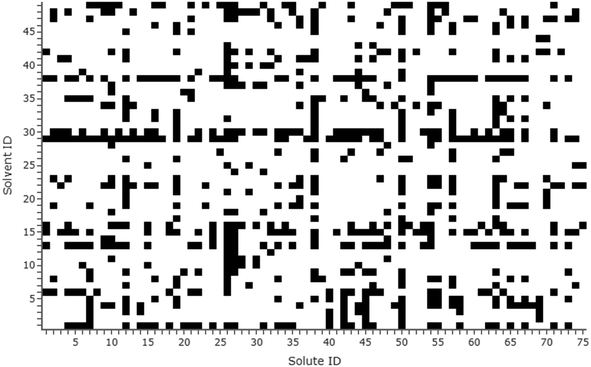Fig. 1 Grid marking the presence of solute/solvent systems in the dataset (black = present). Solute/solvent IDs match those in the dataset (see the ESI†).

For each solute/solvent system present, solubility calculations were carried out with COSMOthermX (release 17) using parameterization BP_TZVPD_FINE_17. Molecular descriptors (2D only) were calculated for each solute and solvent using MOE.³⁴ COSMOthermX and MOE each require licences; the licence type does not affect the output. Apart from removing descriptors with zero variance, no feature selection was performed (RF handles this on-the-fly). All RF models were implemented in R³⁵ using the randomForest³⁶ package. Non-default settings: n_tree = 1000. This was set manually, rather than as a result of a parameter tuning step. It has been suggested that a minor performance gain could be made by increasing n_tree from the default for some datasets^37,38 – while this is by no means a generalisation to all datasets, the only downside to this modest raise of n_tree was computation time, which was manageable for this work. Further external R packages were utilized to carry out this work: dplyr,³⁹ doParallel,⁴⁰ and foreach.⁴¹ All plots were produced with plotly⁴² for R.

For comparison to the DrugBank,⁴³ the 2022 dataset was downloaded and the same MOE descriptors were calculated for all 9694 drug molecules that were marked as approved, experimental, illicit, investigational, nutraceutical, vet-approved and withdrawn. Features not in the main solubility set were dropped. Prior to performing principal component analysis (PCA), all features were scaled to unit variance and zero-centred. For projecting the solubility dataset into the same space, these scaling and centering factors, as well as the subsequent matrix rotation, were extracted and applied to the solubility dataset.

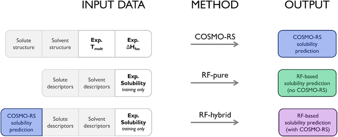
This study examined three different approaches to predicting solubility. The first was the use of standalone COSMO-RS, with no supplementary ML elements, serving as a baseline performance to measure the others against. The second used RF to predict solubility using molecular descriptors from MOE alone (termed RF-pure throughout). This represented a purely data-driven approach, most similar to the efforts of Mitchell and Palmer.²² This method did not require output from COSMO-RS, and so did not require calorimetric data. For this reason, while not equivalent to COSMO-RS, it was the closest to a “competitive” method within the context of this study. The final approach merged the previous two, utilizing COSMO-RS solubility predictions as a descriptor for RF, as well as the set of molecular descriptors from MOE (termed RF-hybrid throughout). In practice, this was a trivial modification to the model, though it meant a significant shift from a purely data-driven alternative to COSMO-RS to a hybrid model. To simplify comparisons between approaches, calorimetry data were not included as descriptors in any datasets used for ML; any differences in performance between RF-pure and RF-hybrid could thus be ascribed to the presence/absence of COSMO-RS output. Fig. 2 summarises the data inputs/outputs of each approach.

Fig. 2 Data inputs and outputs for each prediction method. Notably, RF-pure was independent of COSMO-RS, and so did not ultimately require experimental calorimetry measurements for use, while RF-hybrid required COSMO-RS predictions as input.

Four metrics were used to characterize model performance: R², root mean square error (RMSE), and mean absolute error (MAE), as well as the fraction of cases whose prediction had improved over COSMO-RS, regardless of the magnitude of the improvement (FI). The latter metric was devised as a simple and useful measure of model consistency. By disregarding error magnitude, it contrasted with RMSE, which is by nature particularly sensitive to larger errors. It was intended to provide an indication of risk to the end user for deploying this strategy over simply using COSMO-RS standalone. For example, an FI of 0.5 would mean that as many COSMO-RS predictions were worsened as improved by the applied method (and thus may not be worth applying on an unknown solute), while an FI of 1 would indicate that the method improved all predictions and so could be applied to unknowns with little risk.

Results and discussion

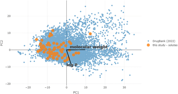
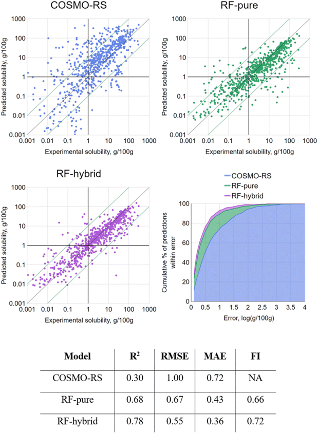
To first put the coverage of chemical space into context, the equivalent molecular descriptors were calculated for the full DrugBank dataset.⁴³ Principal component analysis (PCA) was performed on this set, and the solubility dataset curated for this study was then projected into the same space (details in the Materials and methods). Both sets are overlaid in the first two principal component axes (47% explained variance) in Fig. 3. This is fairly low, but to be expected when attempting to reduce the dimensions of this many molecular descriptors, which are designed to carry non-redundant information. However, the purpose was merely to give a high-level illustration of the diversity of chemical structures in the dataset: it can be seen that the solutes cover the majority of the densely populated space. The accompanying scree plot is included in the ESI.†

Fig. 3 PCA of the DrugBank dataset. The solubility dataset used throughout this study is projected into the same space as a visual estimate of chemical diversity within it. The loadings for molecular weight and log P are displayed to aid in interpretation.

As a first step, 10-fold cross validation (CV) of each of the RF-based approaches was performed to compare against COSMO-RS. The predictions of each fold were merged to produce a set of predictions for the full set and plotted against their associated experimental values (Fig. 4). From the results, both RF-based methods showed a significant improvement over COSMO-RS by all metrics. RF-hybrid outperformed RF-pure, as anticipated, indicating that COSMO-RS predictions were a powerful feature in the dataset. However, due to the composition of the dataset spanning multiple solutes and solvents, it must be highlighted that these results in isolation can create a misleading portrayal of model performance, as discussed below. We retain this conventional train/test splitting methodology as a reference for the rest of this study and comparison with other studies.

Fig. 4 (Upper left) COSMO-RS predictions vs. experimental values; (upper right) the merged 10-fold CV results generated by RF-pure vs. the same experimental values; (middle left) the merged 10-fold CV results generated by RF-hybrid vs. the same experimental values; (middle right) cumulative% of predictions vs. prediction error for each model; (lower) summary metrics for each model.

In randomly partitioning this (or any) dataset, an assumption is made that all data points within are independent of each other, and it is therefore insignificant into which partition they are placed; at least, that is the hypothesis being tested. With this dataset's structure, where each case is a system composed of two distinct molecular property sets (solute and solvent), the assumption is false. If a model has “seen” a solute and/or solvent many times across different systems in its training set, it is likely to make a more accurate prediction for a further system containing it. Equally, for a system of a previously unseen solute and/or solvent, it is likely to make a less accurate prediction. With a validation method based on random partitioning of the dataset, it is overwhelmingly likely that most solvents and solutes spread across both training and testing sets, even with the sparse representation of any individual solute or solvent in this dataset. The 10-fold CV remains a legitimate test, though in this case it models only one scenario that is relevant to an industrial context: where a number of solubility points for a given compound is already known, and the prediction of further points for the same compound is desired. It certainly does not model another, perhaps more likely scenario: where a new compound is being investigated, with zero available solubility data for it.

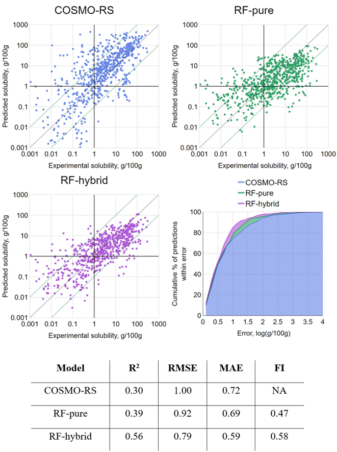
In order to model the latter scenario, a variant of CV was performed where, rather than randomly splitting the data into k equally sized folds, they were split into folds containing all data points for a single solute only. This could be termed “leave-one-solute-out” cross-validation (LOSO-CV). By this approach, all tested data points were treated as previously unseen solutes, with predictions made based only on the remaining solutes in the dataset. Of course, this did nothing to control the distribution of solvents across partitions, but this was considered acceptable given the relatively less likely occurrence of a new solvent being utilized in an industrial context. The results of LOSO-CV are presented in Fig. 5.

Fig. 5 (Upper left) the initial COSMO-RS predictions vs. experimental values; (upper right) the merged LOSO-CV results generated by RF-pure vs. the same experimental values; (middle left) the merged LOSO-CV results generated by RF-hybrid vs. the same experimental values; (middle right) cumulative% of predictions vs. prediction error for each model; (lower) summary metrics for each model.

By LOSO-CV, RF-pure achieved barely better performance metrics than the original COSMO-RS predictions. With FI < 0.5, it was actually more likely to return a prediction with higher error than COSMO-RS. Overall, its performance was not a reliable improvement on COSMO-RS. However, a slight improvement over COSMO-RS was seen with RF-hybrid by all metrics, suggesting that it is theoretically worth applying RF-hybrid to enhance COSMO-RS predictions, even for “new” solutes, leaving aside the overhead of setting up this method.

The strong RF performance by 10-fold CV and the subsequent drop by LOSO-CV indicate that, for a given solute, at least some prior knowledge of its solubility in other systems is significantly helpful for enhancing COSMO-RS predictions. While this is not in itself surprising, it is noteworthy that the relatively simple technique of RF-hybrid was indeed sufficient to exploit this relational information.

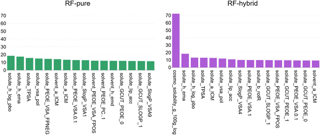
Feature importance analysis was performed using the built-in method for RF. This operates after model training is complete by permuting each feature in turn and re-predicting all out-of-bag validation data. The % increase in MSE is tracked: the more the feature was utilised by the model, the larger this value should be. A dedicated discussion of this analysis, including its limitations, is provided by Gregorutti et al.⁴⁴ and references therein. The results for RF-pure and RF-hybrid (both retrained using the full dataset) are shown in Fig. 6. While the results should only be interpreted coarsely and qualitatively, the analysis yields some useful insights. First, COSMO-RS appears to be the most important feature by far in RF-hybrid. To properly quantify the impact of a single feature on model performance, one would have to retrain an equivalent model having excluded it from the beginning and compare errors. While this has not been carried out for all features, this is precisely the difference between RF-pure and RF-hybrid.

Fig. 6 Feature importance analysis for RF-pure and RF-hybrid (top 16 features shown in both cases).

COSMO-RS aside, most of the highly ranked features describe the solute rather than the solvent in both cases. This is likely due to there being a greater variety of solutes than solvents (75 vs. 49), and so more variance in solute features. The features themselves describe a range of molecular properties one might expect to be important for characterising solubility, including hydrogen bonding, surface area, partial charges, molecular size and rotatable bonds. The full feature set is described in the MOE manual.³⁴ A deeper analysis of the features' contributions to the models was not entered into here, since the models were far from perfect and likely to significantly change in future as more experimental data are obtained. It was more relevant to real-world applications to focus on the impact of additional experimental data. For interested readers, the highest-error predictions of both COSMO-RS and RF-hybrid are listed in the ESI.†

Given the observed drop in model performance for unseen solutes, it was relevant to ask how much prior knowledge of a solute was needed to bring performance back in line with that achieved by 10-fold CV, since this appeared to be a significant improvement over COSMO-RS.

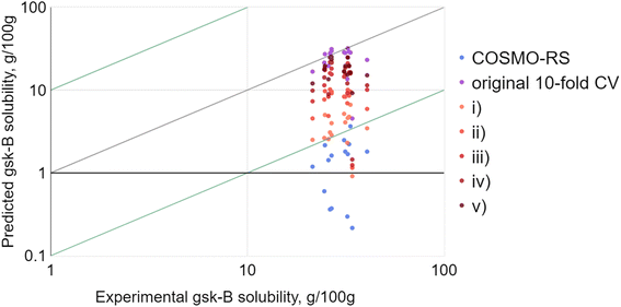
As a test case, one of the solutes provided by GlaxoSmithKline was selected, termed gsk-B. This choice was due to there being experimental solubility data available for a large number of solvents (20 in total). Four of these – ethanol, acetone, 2-propanol and heptane – were held aside and selected as arbitrary common solvents. The solubility of gsk-B in the remaining 16 solvents was predicted by RF-hybrid: (i) given no prior gsk-B solubility data, (ii) given gsk-B solubility in ethanol, (iii) given gsk-B solubility in ethanol and acetone, (iv) given gsk-B solubility in ethanol, acetone and 2-propanol, and (v) given gsk-B solubility in ethanol, acetone, 2-propanol and heptane. This sequence simulated a scenario where single solubility measurements would be obtained experimentally and fed back to the model in order to refine further predictions. The result (Fig. 7) was a consistent improvement with each successive point, with the RMSE matching that of the original 10-fold CV by the third solvent. This was significant: at least in this one case, only a small number of experiments were needed to significantly improve solubility prediction for the same solute.

Fig. 7 RF-hybrid solubility predictions for gsk-B across 16 solvents, (i) given no prior gsk-B solubility data, (ii) given gsk-B solubility in ethanol, (iii) given gsk-B solubility in ethanol and acetone, (iv) given gsk-B solubility in ethanol, acetone and 2-propanol and (v) given gsk-B solubility in ethanol, acetone, 2-propanol and heptane. These are compared against the initial COSMO-RS predictions, as well as the RF-hybrid result achieved by 10-fold CV.

Of course, this example investigated (a) only one solute, (b) only one series of four successive solvents, and (c) only one specific sequence of addition to the training set, so was insufficient for drawing general conclusions. In fact, the moderate improvement seen even with no prior solute data suggested that gsk-B was perhaps a soft choice as an example. However, no single example could ultimately suffice: the logical progression was to investigate all possible combinations – every solute, every set of solvents, and every sequence of addition of that set – and aggregate the results.

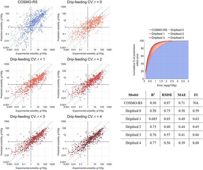
This was achieved by deploying a comprehensive, brute-force cross-validation, drip-feeding all possible combinations of data points of a given solute to training sets, retraining and retesting each time. The procedure, hereafter referred to as “drip-feeding” CV, is described in further detail in the ESI.† Through manual consideration of both the dataset composition and the computational cost required to process exponentially increasing numbers of models, it was decided to perform the drip-feeding CV only on solutes of 5 of more instances in the dataset (57 out of 75). Solutes with fewer instances were omitted, though were retained in training sets. This totalled 169 830 individual RF models.

As a result of this sweep of training/testing combinations, it was possible to aggregate the predictions. For a given value r, where r = the number of times the model had seen solute i in its training set, the results were averaged for each solute/solvent system. This allowed for the production of analogous results to those shown for gsk-B in Fig. 7 for all solutes, all solvent choices and all sequences: the aggregated results are presented in Fig. 8, with a clear trend. When r = 0, the train/test data split resulted in an equivalent test to LOSO-CV, and indeed proved near-identical by all metrics. On increasing to r = 1, where a single solubility measure of the test solute in a different solvent was added to the training set, a significant jump in performance was observed by all metrics. Further increases of r, corresponding to further solubility measures of the test solute present in the training set, resulted in a steady performance enhancement. When r = 4 the model closely matched increases of r, corresponding to further solubility measures of the test solute present in the training set, resulting in a steady performance enhancement. When r = 4 the model closely matched the initial strong performance seen by the 10-fold CV. This finding revealed the merit of an iterative approach to solubility prediction: coordinating with experimentalists and carrying out a small number of targeted measurements could vastly improve modelling capabilities on the remainder.

Fig. 8 The results of drip-feeding CV for RF-hybrid, for r values of 0 to 4. Each point represents the mean prediction error for the given system from all possible training set combinations. Predictions were only made for solutes appearing in the dataset 5+ times to keep the plots comparable (658 of 714 instances). COSMO-RS prediction errors were recalculated for this subset for reference.

A small number of outlier points are visible in Fig. 8 that did not improve as more solute data are made available. These were checked for transcription errors, but have not been further investigated here. However, this approach could possibly be exploited in other applications as an outlier detection technique by tracking prediction errors against the number of training data points.

For reference, drip-feeding CV was also performed for RF-pure, with the expected outcome: a similar overall trend to the above, but with a greater overall error by all metrics. This is presented in the ESI.†

True like-for-like performance comparisons with other ML-based solubility models are challenging, given the ability of this approach to exploit data relationships across solvents, including further ones of a tested solute, and differing input requirements (e.g. utilizing COSMO-RS requires calorimetry data). However, the “headline” error rates can at least be broadly compared with those of some recent alternative ML-based approaches (Table 1). The cross-solvent study by Ye and Ouyang¹⁴ ought to be considered here as well, which reports a RMSE of 0.77 for unseen solutes; however, their dataset could not be retrieved for comparison at the time of writing. Certainly, it is clear that the approach described here extends the level of solubility prediction typical of exclusively aqueous (or other single solvent) models to a vast range of organic solvents while requiring only a small fraction of the number of data points per solvent.

Table 1 Comparison of performance metrics and datasets for a selection of recent solubility prediction studies from the literature. The values representing this study are taken from the drip-feeding CV, where the number of same-solute data points in the training set was controlled

Ref.	Model domain	RMSE	R ^2	No. same-solvent data points in set	No. same-solute data points in set	Total data points in set
11	Water	0.67	0.81	829	0	829
12	Water	0.88	0.45	85	0	85
13	Water (narrow solubility range)	0.71	0.76	560	0	560
13	Water (wide solubility range)	0.71	0.93	900	0	900
13	Ethanol	0.79	0.53	695	0	695
13	Benzene	0.54	0.75	464	0	464
13	Acetone	0.83	0.42	452	0	452
This study	49 solvents	0.75–0.56	0.58–0.77	Max 51, median 10	0–4	714

---

Conclusions

The first goal of this work was to evaluate the use of a single, cross-solvent model to predict solubility across a wide range of systems. Varying both the solute and solvent introduced a new layer of complexity for the model, but also valuable relational information across solvents. It allowed the inclusion of small numbers of data points for given solvents, themselves insufficient for training a solvent-specific prediction model. A further goal was to examine the benefit of a pre-existing, mechanistic solubility prediction (COSMO-RS) included as a feature for the data-driven method (RF).

The cross-solvent approach also introduced complexity regarding validation techniques, since cases were no longer fully independent of one another. A standard 10-fold CV boasted a significant improvement over COSMO-RS for both RF-pure and RF-hybrid. While legitimate, this test did not control the harnessing of same-solute data points in the training set. The effect of controlling for this was demonstrated by LOSO-CV, where train/test data partitions were chosen to isolate each solute in turn. This forced the RF-based methods to treat all test data as unseen solutes, mimicking a more relevant use case in the pharmaceutical industry. Unsurprisingly, performance was hindered. RF-pure did not convincingly outperform COSMO-RS by LOSO-CV. RF-hybrid retained a minor overall improvement in the same test, indicating some innate capacity for RF to enhance COSMO-RS even with no available solubility data for a given solute. This is significant, since the enhancement could be applied with little risk to any COSMO-RS prediction, even with no prior knowledge of the solute, and will likely only improve with a larger dataset.

The disparity between 10-fold CV and LOSO-CV was interrogated further. 10-fold CV disregarded the effect of possessing training data on the same solute being tested, which was not satisfactory, while LOSO-CV only controlled this by forbidding it entirely. However, it was possible to retain control of this extra information while drip-feeding access to it, allowing the effect to be quantified. It required a novel (to the best of the authors' knowledge), brute force method that, for each solute in turn, tested all combinations of training sets containing it on all further instances of the same solute, up to 4 instances in training sets. The final results after pooling the correct subsets were stark: they showed the stepwise gain in predictive power that could be expected for any given solute as experimental measurements of it in other solvents became available. Even a single experimental solubility measurement in a different solvent to the one of interest was enough to significantly improve RF-hybrid over its “blind” LOSO-CV performance. Crucially, this gain is exclusively available to data-driven approaches working on a cross-solvent basis.

Overall, the use of a sparsely populated, cross-solvent dataset to enhance COSMO-RS solubility predictions proved successful, achieving a RMSE of 0.75 log S for previously unseen solutes but, significantly, reducing to 0.65 when one instance of prior knowledge was available, and continuing down to 0.56 when four were available. For reference, COSMO-RS achieved a RMSE of 0.97 across the same dataset. This finding indicates that, where possible, an iterative approach to solubility screening would be optimal for model accuracy, feeding back results as they are generated in order to refine all remaining predictions. For the dataset used in this study, results saw continuing (though diminishing) improvements for up to four instances of a solute in the training set, predicting a correction for a fifth.

This work focused on truly getting the most out of the “hard currency” of experimental data in terms of predictive capability. Alternative models to COSMO-RS and RF were not investigated, and neither were alternative descriptor sets to MOE. The strategy used was intentionally agnostic with respect to these components: operators could freely swap any/all of them for their preferred techniques and the analyses performed here would remain valid, revealing equivalent parts of the story for the new setup.

Finally, it is worth adding that the very fact that RF-hybrid emerged significantly superior to RF-pure at every turn demonstrated the impact of the only difference between them: the incorporation of COSMO-RS output. It hints at the enduring value of mechanistic models in general; COSMO-RS was selected for this study for practical reasons rather than anything fundamental and is just one example. Models like this encapsulate vast quantities of expert human knowledge, often with years and decades of refinement contained within their outputs. Even when inaccurate for a particular system, the information they contribute to a dataset is quantifiably valuable, and, as demonstrated here, certainly not replaceable by simplistic, ML-friendly molecular descriptors.

Data availability

The code for all model training and analysis, along with a processed version of the non-confidential portion of the dataset that is ready for use with the code, is available at https://github.com/AntonyVass/cmac_solpred_cosmo_rf. A release of the source code can also be found at https://doi.org/10.5281/zenodo.6380901. A fully referenced version of the dataset (i.e. citation per measurement of solubility, enthalpy of fusion and melting point) is also provided in the ESI.†

Author contributions

A. D. V. conceptualization, formal analysis, investigation, methodology, software, visualization and writing – original draft; M. N. R. conceptualization, data curation, formal analysis, software, visualization and writing – review & editing; B. G. W. data curation, resources, software; M. S. data curation, resources; S. O. resources; A. J. F. conceptualization, funding acquisition, supervision and writing – review & editing; T. H. conceptualization, data curation, supervision, validation, writing – review & editing; B. F. J. conceptualization, funding acquisition, project administration, supervision, writing – review & editing.

Conflicts of interest

There are no conflicts to declare.

Acknowledgements

The authors would like to thank the EPSRC for funding this work through ARTICULAR: ARtificial inTelligence for Integrated ICT-enabled pharmaceUticaL mAnufactuRing (Grant Ref. EP/R032858/1), Future Continuous Manufacturing and Advanced Crystallisation (CMAC) Research Hub (Grant Ref. EP/P006965/1) and Doctoral Training Centre in Continuous Manufacturing and Crystallisation (Grant Ref. EP/K503289/1). The authors would also like to acknowledge and thank CMAC colleagues Samantha Wilson, Corin Mack and Lennart Ramakers (Grant Ref. EP/P006965/1); Thomas McGlone and Francesca Perciballi (Grant Ref. EP/I033459/1) for sharing and allowing the reuse of experimental solubility measurements from their projects. The authors would finally like to thank GlaxoSmithKline for allowing the internal use of their data, as well as their enthusiastic support throughout this work.

References

1. J. Qiu and J. Albrecht, Org. Process Res. Dev., 2018, 22, 829–835.
2. L. J. Diorazio, D. R. J. Hose and N. K. Adlington, Org. Process Res. Dev., 2016, 20, 760–773.
3. D. Hsieh, A. J. Marchut, C. Wei, B. Zheng, S. S. Y. Wang and S. Kiang, Org. Process Res. Dev., 2009, 13, 690–697.
4. J. Alsenz and M. Kansy, Adv. Drug Delivery Rev., 2007, 59, 546–567.
5. J. G. Hoffer, A. B. Ofner, F. M. Rohrhofer, M. L. Lovrić, R. Kern, S. Lindstaedt and B. C. Geiger, Weld. World, 2022, 2022, 1–14.
6. A. Llinas, I. Oprisiu and A. Avdeef, J. Chem. Inf. Model., 2020, 60, 4791–4803.
7. B. Tang, S. T. Kramer, M. Fang, Y. Qiu, Z. Wu and D. Xu, J. Cheminf., 2020, 12, 15.
8. S. Chinta and R. Rengaswamy, Ind. Eng. Chem. Res., 2019, 58, 3082–3092.
9. A. Avdeef, ADMET DMPK, 2020, 8, 29–77.
10. A. L. Perryman, D. Inoyama, J. S. Patel, S. Ekins and J. S. Freundlich, ACS Omega, 2020, 5, 16562–16567.
11. M. Lovrić, K. Pavlović, P. Žuvela, A. Spataru, B. Lučić, R. Kern and M. W. Wong, J. Chemom., 2021, 35, e3349.
12. D. S. Palmer and J. B. O. Mitchell, Mol. Pharm., 2014, 11, 2962–2972.
13. S. Boobier, D. R. J. Hose, A. J. Blacker and B. N. Nguyen, Nat. Commun., 2020, 11, 5753.
14. Z. Ye and D. Ouyang, J. Cheminf., 2021, 13, 1–13.
15. A. Fredenslund, R. L. Jones and J. M. Prausnitz, AIChE J., 1975, 21, 1086–1099.
16. A. Klamt, J. Phys. Chem., 1995, 99, 2224–2235.
17. V. Papaioannou, T. Lafitte, C. Avendaño, C. S. Adjiman, G. Jackson, E. A. Müller and A. Galindo, J. Chem. Phys., 2014, 140, 54107.
18. BIOVIA COSMOtherm, 2020.
19. A. Klamt, Wiley Interdiscip. Rev.: Comput. Mol. Sci., 2011, 1, 699–709.
20. A. R. Katritzky, Y. Wang, S. Sild, T. Tamm and M. Karelson, J. Chem. Inf. Comput. Sci., 1998, 38, 720–725.
21. W. L. Jorgensen and E. M. Duffy, Adv. Drug Delivery Rev., 2002, 54, 355–366.
22. D. S. Palmer, N. M. O'Boyle, R. C. Glen and J. B. O. Mitchell, J. Chem. Inf. Model., 2007, 47, 150–158.
23. J. Qiu, J. Li, J. Albrecht and J. Janey, Org. Process Res. Dev., 2021, 25, 75–81.
24. D. Rogers and M. Hahn, J. Chem. Inf. Model., 2010, 50, 742–754.
25. S. Boobier, Y. Liu, K. Sharma, D. R. J. Hose, A. J. Blacker, N. Kapur and B. N. Nguyen, J. Chem. Inf. Model., 2021, 61, 4890–4899.
26. M. Orlandi, M. Escudero-Casao and G. Licini, J. Org. Chem., 2021, 86, 3555–3564.
27. M. Lovrić, R. Meister, T. Steck, L. Fadljević, J. Gerdenitsch, S. Schuster, L. Schiefermüller, S. Lindstaedt and R. Kern, Adv. Model. Simul. Eng. Sci., 2020, 7, 1–16.
28. T. Zhang, W. Chen and M. Li, Biomed. Signal Process. Control, 2017, 31, 550–559.
29. A. Correa Bahnsen, D. Aouada, A. Stojanovic and B. Ottersten, Expert Syst. Appl., 2016, 51, 134–142.
30. P. Probst, M. N. Wright and A. L. Boulesteix, Wiley Interdiscip. Rev. Data Min. Knowl. Discov., 2019, 9, e1301.
31. P. Probst and B. Bischl, J. Mach. Learn. Res., 2019, 20, 1–32.
32. V. Svetnik, A. Liaw, C. Tong, J. C. Culberson, R. P. Sheridan and B. P. Feuston, J. Chem. Inf. Comput. Sci., 2003, 43, 1947–1958.
33. A. Klamt, F. Eckert and W. Arlt, Annu. Rev. Chem. Biomol. Eng., 2010, 1, 101–122.
34. Chemical Computing Group ULC, Molecular Operating Environment, 2020.
35. R Core Team, R: a language and environment for statistical computing, R Foundation for Statistical Computing, Vienna, Austria, 2020, https://www.R-project.org/.
36. A. Liaw and M. Wiener, R News, 2002, 2, 18–22.
37. V. Svetnik, A. Liaw, C. Tong, J. Christopher Culberson, R. P. Sheridan and B. P. Feuston, J. Chem. Inf. Comput. Sci., 2003, 43, 1947–1958.
38. R. Genuer, J. M. Poggi and C. Tuleau-Malot, Pattern Recognit. Lett., 2010, 31, 2225–2236.
39. H. Wickham, R. François, L. Henry and K. Müller, dplyr: a grammar of data manipulation, R package version 1.0.2, 2020, https://CRAN.R-project.org/package=dplyr.
40. Microsoft Corporation and S. Weston, doParallel: foreach parallel adaptor for the ‘parallel’ package, R package version 1.0.15, 2019, https://CRAN.R-project.org/package=doParallel.
41. Microsoft Corporation and S. Weston, foreach: provides foreach looping construct, R package version 1.4.7, 2019, https://CRAN.R-project.org/package=foreach.
42. C. Sievert, Interactive web-based data visualization with R, plotly, and shiny, Chapman and Hall/CRC, Florida, 2018.
43. D. S. Wishart, C. Knox, A. C. Guo, S. Shrivastava, M. Hassanali, P. Stothard, Z. Chang and J. Woolsey, Nucleic Acids Res., 2006, 34, D668–D672.
44. B. Gregorutti, B. Michel and P. Saint-Pierre, Stat. Comput., 2017, 27, 659–678.

---

Footnote

† Electronic supplementary information (ESI) available. See DOI: https://doi.org/10.1039/d2dd00024e

---