Ionization energies of metallocenes: a coupled cluster study of cobaltocene

Abstract

Open-shell transition metal chemistry presents challenges to contemporary electronic structure methods, based on either density functional or wavefunction theory. While CCSD(T) is the well-trusted gold standard for maingroup thermochemistry, the accuracy and robustness of the method is less clear for open-shell transition metal chemistry, requiring benchmarking of CCSD(T)-based protocols against either higher-level theory or experiment. Ionization energies (IEs) of metallocenes provide an interesting test case with metallocenes being common redox reagents as well as playing roles as redox mediators and cocatalysts in redox catalysis. Using highly accurate ZEKE-MATI experimental measurements of gas phase adiabatic (5.3275 ± 0.0006 eV) and vertical (5.4424 ± 0.0006 eV) ionization energies of cobaltocene, we systematically assessed the accuracy of the local coupled-cluster method DLPNO-CCSD(T) with respect to geometry, reference determinant, basis set size and extrapolation schemes, PNO cut-off and extrapolation, local triples approximation, relativistic effects and core–valence correlation. We show that PNO errors are controllable via the recently introduced PNO extrapolation schemes and that the expensive iterative triples (T₁) contribution can be made more manageable by calculating it as a smaller-basis/smaller PNO-cutoff correction. The reference determinant turns out to be a critical aspect in these calculations with the HF determinant resulting in large DLPNO-CCSD(T) errors, likely due to the qualitatively flawed molecular orbital spectrum. The BP86 functional on the other hand was found to provide reference orbitals giving small DLPNO-CCSD(T) errors, likely due to more realistic orbitals as suggested by the more consistent MO spectrum compared to HF. A protocol including complete basis set extrapolations with correlation-consistent basis sets, complete PNO space extrapolations, iterative triples- and core–valence correlation corrections was found to give errors of −0.07 eV and −0.03 eV for adiabatic- and vertical-IE of cobaltocene, respectively, giving close to chemical accuracy for both properties. A computationally efficient DLPNO-CCSD(T) protocol was devised and tested against adiabatic ionization energies of 6 different metallocenes (V, Cr, Mn, Fe, Co, Ni). For the other metallocenes, the iterative triples (T₁) and PNO extrapolation contributions turn out to be even more important. The results give errors close to the experimental uncertainty, similar to recent auxiliary-field quantum Monte Carlo results. The quality of the reference determinant orbitals is identified as the main source of uncertainty in CCSD(T) calculations of metallocenes.

---

1 Introduction

Metallocenes are organometallic compounds featuring a metal ion coordinated to two aromatic cyclopentadienyl (Cp) rings, being a subset of the larger category of sandwich compounds (see Fig. 1). The discovery of ferrocene in 1951 is commonly referred to as the starting point of modern organometallic chemistry.¹ Today, metallocenes form a large family of compounds, which are still very relevant to many fields of chemistry. They commonly undergo one or more reversible one-electron oxidations, or even reduction. Each Cp ring has 5 sites which can be substituted by R-groups, allowing for tuning of their properties. Ferrocene, for example, has been conjugated to amino-acids, peptides or DNA,² and is commonly used as an internal reference in electrochemistry.³ Metallocenes also play a role in catalysis, with zirconocenes being prevalent in catalytic olefin polymerization.⁴ and decamethylchromocene and cobaltocene being common reducing/oxidation agents, including the field of N₂ activation chemistry.^5–7 Cobaltocene (Cp₂Co) and its derivatives can even be protonated and become capable of concerted proton–electron transfer (CPET)^8,9 chemistry, enabling them to act as redox mediators for N₂ and CO₂ fixation^10,11 More recently, Peters and coworkers have shown that cobaltocene derivatives with a tethered Brønsted base can act as particularly useful CPET mediators when combined with molecular catalysts, bypassing the competing hydrogen evolution reaction, enabling efficient H-atom addition steps for reducing unsaturated organic molecules^12,13 and remarkably even fixing N₂.¹⁴

Fig. 1 Cobaltocene (Cp₂Co) in the eclipsed D_5h conformer and a qualitative MO diagram of the ground state.

In order to improve rational design and tuning of metallocene properties using theoretical methods, a thorough understanding of their electronic structure and redox chemistry is necessary, requiring computational methods that can describe them consistently.

Unlike density functional theory, wave function theory (WFT) methods form a systematic approach towards approaching the solution of the exact electronic Schrödinger equation. Single-reference wavefunction theory in the form of the coupled cluster expansion is a particularly successful strategy. Electron correlation is included in the wavefunction by including excited Slater determinants via the exponential excitation operator. The excitation operator is in practice truncated early and the most common truncation includes singles and doubles (CCSD) with triples included perturbatively: CCSD(T). The CCSD(T) method is commonly discussed as the “gold standard” of computational chemistry and more approximate methods are often benchmarked against CCSD(T), particularly in the absence of reliable experimental data.^15–17

A drawback of the canonical CCSD(T) method is the N⁷ scaling with system size. Fortunately, great advances have been made in the past decade with the development of near linear scaling local correlation methodology. A pioneering method is the domain based local pair natural orbital couple cluster singles doubles and pertubative triples (DLPNO-CCSD(T)) approach implemented in ORCA.^18–22 The method aims to retain near-CCSD(T) accuracy at much reduced computational cost by using localization of the occupied orbitals and a truncated unoccupied pair natural orbital (PNO) basis, expanded in terms of projected atomic orbitals (PAOs) in domains. Pre-screening methods based on perturbation theory truncate the PNO space for each electron pair based on a predefined cut-off in their occupation numbers. Taking advantage of 1/R⁶ decay in correlation energy with distance between electron pairs (sparsity), domains are defined and MP2 (or semi-canonical local MP2) correlation energies then decide which pairs are treated with CC (strong pairs), which are treated at the MP2 level (weak pairs) and which are discarded, also based on predefined cut-offs. This allows for a highly compact treatment of electron correlation in the coupled cluster wavefunction. The method originally employed only semi-canonical perturbative triples excitations, denoted T₀, which ignores off-diagonal Fock matrix elements. It was later shown that in some cases, including open-shell metal complexes, this approximation can cause large errors, and a fully iterative triples (T₁) approximation was implemented that more accurately reproduces canonical triples correlation energies.²³

Despite the overwhelming success of coupled cluster theory and local correlation substantially extending the domain of applicability, the ability of CCSD(T) to accurately describe transition metal compounds, especially open-shell compounds, has sometimes been called into question.^24,25 Such problems have often been attributed to the multi-reference character of transition metal complexes, see e.g. ref. 26 for a discussion. Truhlar and coworkers, for example, concluded that the CCSD(T) method is no more accurate than the best available density functional approximations in predicting heats of formation for a group of transition metal diatomics, and suggested suspending the use of CCSD(T) as reference method when benchmarking KS-DFT,²⁴ while Peterson and coworkers reported that CC methods do, in fact, outperform DFT methods for the same data set (revised experimental values used for some species) and for metal oxide monomers and dimers.^27,28 However, studies on diatomic molecules or other very small metal complexes may also represent particularly difficult examples (probably more prone to multireference effects) and are perhaps not representative of the ligand fields more commonly encountered in synthetic inorganic and organometallic chemistry.

Recently, Friesner and coworkers performed a computational study into the ionization energies (IEs) of a group of metallocenes for which experimental data were available, benchmarking DFT methods, DLPNO-CCSD(T) as well as their auxiliary field quantum Monte Carlo method (AFQMC).²⁹ Remarkably they found that a DLPNO-CCSD(T₀) protocol was no more reliable than DFT methods. The work did not establish clearly, however, whether this indicates an inherit shortcoming of the coupled cluster method, or whether it is caused by the approximations invoked by the DLPNO methodology.

To clarify this apparent failure of DLPNO-CCSD(T) to accurately describe the IEs of metallocenes, it would be first useful to rule out potential errors from the experimental measurements. The experimental ionization energies were derived from electron–transfer equilibrium experiments using Fourier transform ion cyclotron resonance mass spectrometry at 350 K.^30,31 with reported uncertainties of ±1.5 kcal mol⁻¹ (±0.065 eV). It would be preferable, however, to have access to a truly high resolution determination of the ionization energy of a metallocene at threshold and techniques based on zero kinetic energy (ZEKE) and mass-analyzed threshold ionization (MATI) allow for much lower uncertainties. In these methods, jet-cooled molecules are excited to Rydberg states (ZEKE states), followed by electric pulse ionization, and if the ZEKE states live long enough, this will allow for a high-resolution vibronic-level photoionization spectrum. Such an experiment has only been successful for one unsubstituted metallocene: cobaltocene (Cp₂Co).³² From the photoionization spectrum, adiabatic- and vertical-ionization energies (IEs) of Cp₂Co in the gas phase could be determined with extremely high precision (±0.0006 eV): giving an adiabatic IE of 5.3275 eV and a vertical IE of 5.4424 eV.³² This high-accuracy determination of the ionization energy of cobaltocene at 0 K thus provides an excellent opportunity to thoroughly test electronic structure methods as this experimental reference is free from temperature, entropic and environmental effects and has a much lower experimental uncertainty than data for other metallocenes.

In this work we systematically study the accuracy and convergence of the CCSD(T) method (in its local correlation, DLPNO-form) in calculations of adiabatic- and vertical IEs of Cp₂Co, exploring the dependence of geometry, reference orbitals, relativistic effects, basis set, PNO thresholds, local triples approximations and core–valence correlation effects on the final result. We thoroughly analyze different reference orbitals of Cp₂Co, in an attempt to explain why some KS-DFT reference orbitals outperform others, and to understand the failure of the HF reference orbitals. We test the accuracy of the DLPNO-CCSD(T) method against the highly accurate experimental values when calculated at the highest levels our computational resources allow, as well as suggesting protocols that balance computational cost and accuracy. These protocols were then tested for adiabatic ionization energies of the series of metallocenes, previously studied by Friesner and coworkers, and compared to the results of the gas phase electron-transfer equilibrium experiments^30,31 as well as the previous AFQMC and DLPNO-CCSD(T₀) computations.²⁹

2 Computational details

2.1 DFT calculations

All calculations in this study were carried out using the ORCA quantum chemistry program,^33,34 version 5.0.2, interfaced to the ASH program.³⁵ Geometry optimizations and frequency calculations were performed with the following density functionals: BP86, TPSS, r²SCAN, TPSSh, B3LYP, PBE0, BHLYP and M06-2X.^36–42 PBE and PW91 orbitals were additionally tested as reference determinants in correlation calculations. DFT-D3 dispersion corrections (with Becke–Johnson damping) were included in all cases except for the M06-2X functional.^43–45 D4 dispersion was used for Cp₂Mn for reasons detailed in the text.⁴⁶ Harmonic vibrational frequency calculations were carried out for evaluation of zero-point energies. For vibrational entropies the quasi rigid rotor harmonic oscillator approximation (QRRHO) was used as implemented in ORCA.⁴⁷ All DFT calculations used a def2-TZVP basis set with a decontracted Coulomb fitting auxiliary basis set^48,49 used in the resolution of identity (RI) approximation^50–53 implemented in the SHARK integral library of ORCA.⁵⁴ The RIJCOSX approximation was used for hybrid DFT calculations to approximate HF exchange integrals.^55–58 Very fine integration grids and tight SCF convergence criteria were used (“DefGrid3” and “VeryTightSCF” keywords in ORCA). Optimized structures were confirmed to be local minima by inspection of the calculated Hessian. Stability analysis was performed following all single-point SCF calculations, to verify the stability of the SCF solution. Kohn-Sham reference orbitals in the CC calculations utilized a Douglas–Kroll–Hess (DKH) scalar relativistic Hamiltonian^59–63 along with the relativistically contracted DKH-def2-XVP,^48,64 cc-pVnZ-DK and cc-pwCVnZ-DK^65,66 basis set families. The effect of scalar relativity on IEs compared to nonrelativistic calculations was investigated separately as detailed in the ESI.†

2.2 DLPNO-CCSD(T) calculations

(DLPNO-)CCSD(T)^20,22 calculations were carried out with the DKH relativistic Hamiltonian throughout, using either the relativistic version of the Ahlrichs def2 basis set family,^48,64 with sizes SVP through QZVPP, or the correlation consistent basis sets: cc-pVnZ-DK/cc-pwCVnZ-DK (N = 2, 3, 4, 5).^65,66 An automatically generated auxiliary fitting basis set was used (“AutoAux” option in ORCA with maximum angular momentum option) was used in all CC calculations.⁶⁷ Unless otherwise stated, the DLPNO-CCSD(T) calculations were carried out using the default frozen core approximation as implemented in ORCA,⁶⁸ where 1s electrons of carbon are frozen, but the frozen core of cobalt (and other 3d metals) goes up to the 2p shell (10 electrons). An alternative frozen core strategy was also tested as shown in the ESI.† DLPNO-CCSD(T) calculations used either the semi-canonical (T₀) approximation or the more accurate iterative (T₁) triples.²³ As the full LMP2 guess is only available for closed-shell DLPNO calculations, it was disabled in all calculations in this work. Core–valence (CV) corrections, where all electrons are correlated, were tested using both semi-canonical (T₀) and full iterative triples, (T₁). Several cutoffs control the accuracy (and cost) of the DLPNO approximation with “T_CutPNO”, “T_CutPairs” and “T_CutMKN” being the most important ones. ORCA provides three settings, named “LoosePNO”, “NormalPNO” and “TightPNO” (hereafter referred to as L.PNO, N.PNO and T.PNO) that sets appropriate cutoffs for each accuracy level. The T_CutPNO cutoff is the occupation number below which PNOs are discarded from the virtual space. The T_CutPairs cutoff is the MP2 (or semi-canonical local MP2 (SC-LMP2)) correlation energy below which electron pairs will be treated as weak pairs (MP2 level), while T_CutMKN controls the PNO domain size. The reader is pointed to ref. 20 for further details regarding these thresholds.

2.3 Extrapolations and corrections

Two-point extrapolations of the correlation energies to the complete basis set (CBS) limit were accomplished using eqn (1), as suggested by Helgaker and coworkers,^69,70 where X and Y are the basis set cardinal numbers, D(2), T(3), Q(4), 5 for the cc-pVnZ basis set family and SVP(2), TZVPP(3) and QZVPP(4), for the def2 basis set family. The theoretical value for β is 3, however, it has been shown that 2.4 gives more reliable results for CBS(2/3) extrapolations.^71,72 We have used β = 2.4 in 2/3 extrapolations and β = 3 for larger basis sets.

Similarly, reference energies can be extrapolated to the CBS limit as well. A plot of the reference energy convergence, total and relative energies, can be found in the ESI.† Two extrapolation schemes, originally optimized for HF-SCF energies, were tested but neither was found to perform satisfactorily. This is likely a problem associated with the use non-selfconsistent HF energies evaluated on top of KS-DFT reference orbitals, a strategy primarily used in this work. Therefore, extrapolated CBS energies reported here only rely on CBS extrapolations of correlation energies according to eqn (1), whereas, reference energies (E(ref.)) are HF reference energies on KS-DFT orbitals (transformed to quasi-restricted orbitals⁷³ for the open shell case) using the larger basis set involved in the CBS extrapolation. This means e.g. that a DLPNO-CCSD(T)/CBS(3/4) calculation will use quadruple ζ basis set E(ref.) energies, and CBS(3/4) extrapolated correlation energies from eqn (1).

Following the work of Bistoni and coworkers,⁷⁴ extrapolations of DLPNO-CCSD(T) energies to complete PNO space limit (CPS) were explored. Two-point extrapolations of energies to the CPS limit were carried out using eqn (2), where E^J and E^K are the correlation energies using T_CutPNO = 10^−J and T_CutPNO = 10^−K cut-offs, where K = J + 1.

E(CPS) = E^J + F(E^K − E^J) (2)

A value of F = 1.5 was derived from extensive benchmarking.^74,75 Note that eqn (2) is derived from a similar expression as eqn (1), where several terms have been substituted for the constant F for simplification. We tested both J = 5 and J = 6 in this work; however, J = 5 was deemed unreliable. CPS calculations with J = 6 and K = 7 use T.PNO settings for all other cut-offs in the DLPNO treatment. The final CPS energies can then be used in the CBS extrapolations according to eqn (1). Additionally, a more economical approach to CPS extrapolation was suggested by Drosou and Pantazis.^76,77 In their suggested CPS extrapolation, T_CutPNO values of 10⁻⁶ and 3.33 × 10⁻⁷ are used along with “NormalPNO” settings for all other cutoffs in CPS extrapolations, for which a value of F = 2.38 was derived. This will hereafter be called CPS(1) and using T_CutPNO values of 10⁻⁶/10⁻⁷ and F = 1.5 will be called CPS(2), following the notation of Drosou and coworkers.

Eqn (3) and (4) show how the IE was calculated throughout the article. They vary in terms of sophistication regarding basis set sizes, PNO cut-offs and corrections included depending on the objective of each section:

ΔE = ΔE(ref.) + ΔE(CCSD)^N.PNO_CBS(3/4) + ΔE(T₀)^N.PNO_CBS(3/4) + ΔE(ZPE) (3)

ΔE = ΔE(ref.) + ΔE(CCSD)^CPS(2)_CBS(4/5) + ΔE(T₀)^CPS(2)_CBS(4/5) + ΔE(ZPE) + ΔE(T₁)^CPS(2)_{CBS(3/4)|corr} + ΔE(CV)^CPS(2)_{CBS(3/4)|corr} (4)

where ΔE is always the energy difference between cation and neutral and E(ZPE), zero-point energy correction from DFT harmonic frequency calculations, is only included in calculations of adiabatic IE. E(ref.) is the HF energy using KS-DFT/HF orbitals using the larger basis set in case of a two-point CBS extrapolation.

Eqn (3) shows how the IE is calculated in Section 3.2, where geometries and different reference orbitals are compared. In Section 3.3, calculations of both the vertical and adiabatic IE for Cp₂Co are taken to the limit of our computational resources according to eqn (4) and compared to the aforementioned highly accurate ZEKE-MATI experiments. Furthermore, E(T₁)_corr and E(CV)_corr corrections were explored at several levels of theory with respect to basis set size and PNO cut-offs, the largest being CPS(2) energies in CBS(3/4) extrapolations as shown in the equation. The E(T₁) correction is calculated as E(T₁)–E(T₀) using the same basis set and PNO cut-offs for both E(T₁) and E(T₀), usually at a lower level than E(CCSD) and E(T₀). The correction for correlation of core electrons, E(CV)_corr, is calculated as E(AE)–E(FC), with the same basis set and PNO cut-offs for both energies, where E(AE) is the total energy with all electrons correlated and E(FC) is the energy using the frozen core approximation, as described above. As the relativistic cc-pwCVnZ-DK core–valence basis sets are not available for carbon, they were used only on cobalt and cc-pVnZ-DK on C and H.

In Section 3.4, we calculate the adiabatic IE for comparison with electron-transfer equilibrium experiments, determined at 350 K. This requires the inclusion of thermal and entropic corrections from the harmonic frequency calculations, therefore, ΔE(ZPE) should be replaced by a free-energy correction at 350 K, G_corr. Two protocols, protocol (1) and protocol (2), were tested and are described by eqn (5) and (6), respectively. Protocol (2) is inspired by the work of Pantazis and coworkers and is much more economical than protocol (1).^76,77 In addition to the more economical CPS(1) (described above) energies, the cc-pV(T/Q)Z-DK basis sets are only extrapolated for the metal atom in M-CBS(3/4) extrapolations, while cc-pVTZ-DK is fixed for other atoms. It should also be noted that L.PNO* in eqn (6) refers only to the T_CutPNO = 10⁻⁶, whereas other cut-offs were kept at N.PNO values.

ΔE = ΔE(ref.) + ΔE(CCSD)^CPS(2)_CBS(3/4) + ΔE(T₀)^CPS(2)_CBS(3/4) + ΔG_corr + ΔE(T₁)^N.PNO_{CBS(3/4)|corr} (5)

3 Results and discussion

In Sections 3.1–3.3 we systematically test how the ionization energy of cobaltocene depends on various choices made in a DLPNO-CCSD(T)//DFT computational protocol. Section 3.1 compares the DLPNO error against canonical CCSD(T) for a small basis set, while Section 3.2 discusses the effect of geometry and reference determinant in DLPNO-CCSD(T) calculations. Section 3.3 combines all contributions and compares the final result against the high-accuracy experiment. Finally Section 3.4 discusses the result of a computationally efficient DLPNO-CCSD(T) protocol (based on the results of Sections 3.1–3.3) on a larger test set of experimentally available ionization energies for metallocenes and compares against experiment as well as previous DLPNO-CCSD(T₀) and AFQMC calculations.

3.1 Comparison to canonical CCSD(T)

The accuracy of the DLPNO-CCSD(T) method was first investigated by a systematic comparison against canonical CCSD(T) (with no local approximation) using the small cc-pVDZ-DK basis set and relativistic DKH Hamiltonian. The singles-doubles, E(CCSD), and triples, E(T), correlation energy as well as the ionization energy (IE), calculated with the DLPNO-CCSD(T) method using N.PNO, T.PNO and CPS cut-offs at both T₀ and T₁ levels, is compared to canonical CCSD(T) in Table 1. This comparison allows one to determine at which level the DLPNO approximation adequately approximates canonical CCSD(T) for both the open-shell Cp₂Co and closed-shell Cp₂Co⁺ species, with the only drawback being the small basis set size.

Table 1 Correlation energy contributions of DLPNO- and canonical-CCSD(T) to Cp₂Co and Cp₂Co⁺ with the cc-pVDZ-DK basis set and DKH Hamiltonian^a

	Cp2Co				Cp2Co^+				IE^e [eV]	Δ Can. [meV]
	E SD [Eh]	Δ Can. [mEh]	E(T)^d [Eh]	Δ Can . [mEh]	E SD [Eh]	Δ Can. [mEh]	E(T) [Eh]	Δ Can. [mEh]
a Correlation energies and energy differences are given in Hartree and milliHartree atomic units, respectively. Ionization energies and energy differences are in eV and meV, respectively. b Correlation energy from calculations of singles and doubles excitations. c Difference in energy between a given DLPNO-CCSD(T) protocol and canonical CCSD(T) energies. d Correlation energy from calculations of triples excitations. e Calculated IE, difference in total energy of Cp2Co^+ and Cp2Co. f Canonical CCSD(T) energies. g DLPNO-CCSD(T) energies with varying PNO cut-offs and T0 or T1 triples, as described in Section 2.2. In CPS(2)(T0/T1), the E(T1) correction (Section 2.3) is calculated as E(T.PNO(T1)) − E(T.PNO(T0)), then added to the triples CPS(2)(T0) correlation energy.
CCSD(T)Can^f	−2.1476		−0.1358		−2.1558		−0.1458		4.844
N.PNO(T0)^g	−2.1410	−6.6	−0.1074	−28.4	−2.1487	−7.1	−0.1166	−29.3	4.880	36
T.PNO(T0)	−2.1426	−5.0	−0.1091	−26.7	−2.1505	−5.3	−0.1181	−27.7	4.880	36
CPS(2)(T0)	−2.1465	−1.1	−0.1110	−24.8	−2.1551	−0.7	−0.1199	−25.9	4.863	18
N.PNO(T1)	−2.1410	−6.6	−0.1110	−5.6	−2.1487	−7.1	−0.1403	−5.5	4.856	12
T.PNO(T1)	−2.1426	−5.0	−0.1329	−2.9	−2.1505	−5.3	−0.1428	−3.0	4.854	10
CPS(2)(T1)	−2.1465	−1.1	−0.1357	−0.1	−2.1551	−0.7	−0.1456	−0.2	4.836	−8
CPS(2)(T0/T1)	−2.1465	−1.1	−0.1348	−1.0	−2.1551	−0.7	−0.1446	−1.2	4.837	−7

---

A quasi-restricted reference determinant based on unrestricted BP86 orbitals was used for both DLPNO- and canonical CCSD(T) methods for both closed-shell and open-shell Cp₂Co in order to get a consistent treatment of the 4th-order doubles-triples correlation effect for non-HF references in ORCA. See Section S.5 in the ESI,† for a discussion.

Table 1 shows that the use of N.PNO cutoffs with the default T₀ approximation gives unacceptable errors for both SD and T correlation energies for Cp₂Co and Cp₂Co⁺ species. While the error is systematic and cancels out to some extent in the ionization energy (error of 36 meV), such a cancellation of large individual correlation errors is unlikely to be robust when turning to larger basis set calculations or when studying other systems. Interestingly, while the use of tighter thresholds (T.PNO) with T₀ lowers the errors for both E(SD) and E(T₀) slightly, it does not affect the error in ionization energy. However, the use of PNO extrapolation, CPS(2)(T₀), does lower the error in SD energy to roughly 1 mEh for both Cp₂Co and Cp₂Co⁺, which is within chemical accuracy (1 kcal mol⁻¹ or 1.6 mEh). The error in IE is also lowered from 36 to 18 meV. The error in triples correlation energy, however, is still in the region of 25 mEh from the canonical reference for both species. The iterative T₁ triples method is clearly required for calculations of this system, as evident by the substantial lowering of the error in triples correlation energy to roughly 5.5 mEh for both species in N.PNO(T₁) calculations. In T.PNO(T₁) calculations, the E(SD) and E(T₁) errors are roughly 5 and 3 mEh, respectively, for both Cp₂Co and Cp₂Co⁺, meaning that 99.8 and 97.9% of the respective correlation energies has been captured relative to canonical CCSD(T). The T₁ error is close to zero at the CPS(2)(T₁) level, resulting in total errors in correlation energy within chemical accuracy for both species, capturing >99.9% of the E(SD), and 99.9% of E(T) relative to the canonical reference. While the IE errors are overall modest for all DLPNO protocols in Table 1, a protocol such as CPS(2)(T₁) with DLPNO correlation energy errors for both species in the range of 1 mEh and with a decreased IE error of −8 meV vs. +36 meV (N.PNO(T₀)) is likely to be more robust as it relies on less error cancellation.

Unfortunately, the T₁ iterative triples method is computationally very expensive, especially in open shell calculations, with open-shell species such as neutral Cp₂Co necessarily encountered when calculating ionization energies. Furthermore, PNO extrapolation involves two calculations varying the T_CutPNO parameter. Therefore, a two-point CBS extrapolation, using CPS energies with larger basis sets consists of four expensive correlation calculations for each species. Calculating everything at the T₁ level would thus result in a tremendous increase in computational cost. We therefore, suggest an additive E(T₁) correction to the CPS(2)(T₀) triples correlation energy, calculated here as E(T.PNO(T₁))–E(T.PNO(T₀)) and labeled CPS(2)(T₀/T₁) in Table 1. Deviation from the benchmark in triples correlation energy is close to 1 mEh for both species compared to 0.1–0.2 mEh in the CPS(2)(T₁) calculations, capturing 99.2% of triples correlation compared to 99.9%. The total error in correlation energy using the CPS(2)(T₀/T₁) method is 2.2 mEh and 1.9 mEh for Cp₂Co and Cp₂Co⁺, respectively, and the IE error is only −7 meV. This correction is further explored with respect to basis set size and PNO cut-offs in Section 3.3.

3.2 Geometries and reference orbitals

3.2.1 Geometry optimizations. Geometry optimizations with high level WFT methods are impractical for molecules larger than a few atoms and analytical gradients are only rarely available. It is, nonetheless, essential to choose an appropriate geometry to obtain meaningful results from correlated wavefunction calculations. Metallocenes have two main conformers, staggered D_5d or eclipsed D_5h. Other studies have concluded that the eclipsed D_5h, lowered to C_2v by Jahn–Teller distortion, is the more stable conformer of cobaltocene, which is consistent with our results.^78–80 The structure and a qualitative MO diagram of the ground state can be seen in Fig. 1. The D_5h representation will be used for neutral Cp₂Co here for sake of comparison to the cation, which is closed-shell and, therefore, does not suffer from Jahn–Teller distortion.

Geometries of Cp₂Co and Cp₂Co⁺ were optimized with several density functionals, always including D3 dispersion. The results are summarized in Table 2. The optimized geometries for neutral Cp₂Co are compared to experimental values, obtained from gas phase electron diffraction (GED) measurements.⁸¹ The average Co–C and C–C distances were chosen as they had the lowest experimental uncertainties (±0.3 pm), and because the Co–C distance likely has the largest impact on the IE. The average Co–C distances for the Cp₂Co⁺ cation are also listed in the table along with the change in the average Co–C distance upon ionization, Δ_Co–C. No experimental data on the cation structure is available. Structures obtained with r²SCAN and BHLYP were not included in the table as we were unable to optimize the r²SCAN structure to a minimum; it would always converge to a saddle-point along the Jahn–Teller active vibrational mode. BHLYP, on the other hand, would only converge to the staggered, D_5d, conformer.

Table 2 Average Co–C and C–C distances of Cp₂Co in DFT-optimized geometries using def2-TZVP basis set and D3 dispersion correction, compared to experimental values^a

	Cp2Co		Cp2Co^+
	r Co−C	r C−C	r Co−C	ΔrCo−C
a All units are in pm. Errors relative to experiment are shown in parentheses. experimental GED values are not corrected for thermal motion. b No dispersion correction was used for M06-2X.
Expt.	211.2	143.0
BP86-D3	210.7 (−0.5)	143.2 (0.2)	204.7	−6.0
TPSS-D3	209.7 (−1.5)	143.0 (0.0)	203.7	−6.0
TPSSh-D3	210.0 (−1.2)	142.5 (−0.5)	203.4	−6.6
B3LYP-D3	214.2 (3.0)	142.2 (−0.8)	206.2	−8.0
PBE0-D3	211.2 (0.0)	141.8 (−1.2)	203.5	−7.7
M06-2X^b	223.6 (12.4)	141.6 (−1.4)	209.2	−14.4

---

BP86, TPSS and TPSSh capture the C–C bond length of the neutral to within 0.5 pm. DFAs with higher fractional HF exchange than TPSSh predict shorter C–C bonds, with errors increasing systematically with the amount of HF exchange, where M06-2X (54% HF exchange) has the largest error in C–C distance, −1.4 pm. For the Co–C distance, PBE0 and BP86 perform the best, having errors of 0.0 and 0.5 pm, respectively. This is consistent with previous results in the literature, reporting good agreement with experiment for BP86 and PBE0 metallocene geometries.^80,82 Radoń and coworkers further showed that deviations over 1 pm in M-Cp distance resulted in significant errors in excitation energies, and recommended reproducing experimental M-Cp distances to within that value.⁷⁹ Such a cutoff would exclude all geometries tested here apart from BP86 and PBE0; although IEs may not be as sensitive as excitation energies in this comparison. It should be noted, however, that the GED geometries were not corrected for thermal motion. For ferrocene, the Fe–C distance corrected for thermal motion is 1 pm shorter than the GED value.⁸³ If one were to assume similar behaviour for Cp₂Co would suggest that BP86, TPSS, and TPSSh have the most accurate description of the Co–C distance.

Upon oxidation of Cp₂Co, all DFAs predict a contraction of the Cp rings towards the Co center, i.e. shortening the Co–C distance. This is not unexpected, as the neutral complex has a doublet ground state with an unpaired electron in the d_xz/yz orbitals, which have π anti-bonding character with the Cp rings (Fig. 1 and 6). GGA functionals predict a 6 pm shortening of the Co–C distance; the hybrids, however, especially with higher HF exchange, predict even greater contraction of the Cp rings. Most noteworthy here, is that the best performing methods for the neutral – PBE0 and BP86 – differ by 1.2 pm for the Co–C distance of the cation, Cp₂Co⁺.

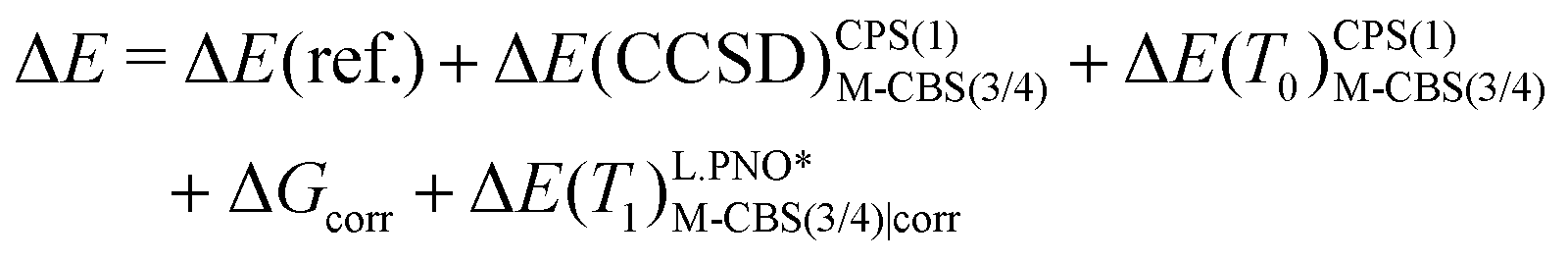
The lowest total energies using WFT methods evaluated on different geometries, have sometimes been used as criteria in distinguishing geometries calculated at lower levels of theory.^80,84 This would present complications here, however, as several reference determinants can be considered in addition to geometries and coupled cluster theory not being variational. The total energies of each geometry were first compared in crude DLPNO-CCSD(T₀) calculations in CBS(2/3) extrapolations and BP86 reference orbitals. From these, the BP86-D3, TPSSh-D3 and PBE0-D3 geometries were chosen for calculations of adiabatic- and vertical-IEs, in CBS(3/4) extrapolations, as described by eqn (3). BP86 was included for having the best overall geometry compared to experiment, whereas PBE0 had the lowest CBS(2/3) total energies. TPSSh, on the other hand, had the lowest energy at both cc-pVDZ-DK and cc-pVTZ-DK levels, although the CBS(2/3) extrapolation gave slightly higher energies than PBE0. To exclude any bias, all three Kohn-Sham references were used in IE calculations on all geometries. The results can be seen compared to the ZEKE-MATI experimental values in Fig. 2. All adiabatic IEs include ZPE contributions from the functional corresponding to the geometry in each case (see ESI†).

Fig. 2 Adiabatic- (top) and vertical- (bottom) ionization energies of Cp₂Co calculated with DLPNO-CCSD(T₀) on three geometries with three different reference orbitals. The geometry is labeled at the bottom by the x-axis, BP86, TPSSh and PBE0 from left to right (D3 dispersion was always included). The DFAs used as reference orbitals are color coded, where blue is BP86, red is TPSSh and green is PBE0. The colored lines represent IEs calculated with cc-pVTZ-DK and cc-pVQZ-DK basis sets and the squares show the IE calculated in CBS(3/4) extrapolations. The dashed line represents the experimental IEs. The DKH relativistic Hamiltonian and N.PNO cut-offs were used throughout.

In the case of the adiabatic IE, all reference orbitals give the lowest error relative to experiment using the BP86-D3 geometries. Moreover, using BP86 reference orbitals results in the lowest error for all three geometries. Using the BP86-D3 geometry, the BP86 reference gives an error of −28 meV, while both TPSSh and PBE0 references have errors of −44 meV. For the TPSSh-D3 geometry, the IE remains unchanged with the BP86 reference, whereas the errors have increased to 49 and 55 meV using TPSSh and PBE0 references, respectively. The largest errors for all references were observed on the PBE0-D3 geometry, being 46, 60 and 69 meV for BP86, TPSSh and PBE0, respectively. It should be noted that the ΔE(ZPE) contribution to the IE was taken for each functional based on geometry, contributing +1 meV to the observed differences in adiabatic IE between BP86-D3 and TPSSh-D3 geometries, and −6 meV between BP86 and PBE0.

The vertical IEs are reproduced very well using any of the reference methods on both BP86-D3 and TPSSh-D3 geometries. All errors are smaller than 10 meV on the BP86-D3 geometry, the largest one being 8 meV with the BP86 reference. At the TPSSh-D3 geometry, the errors increase slightly for all references, the largest error being with the TPSSh reference, −21 meV. The largest errors in vertical IEs for all references are also on the PBE0-D3 geometry, just as observed for the adiabatic case, in the opposite direction, however. For BP86 reference orbitals, the error increases to 53 meV, and to 38 and 39 meV for TPSSh and PBE0, respectively.

Information on the quality of the neutral geometry can be inferred from the vertical IEs, as it is the only geometry used in the calculations. The results suggest better geometries of neutral Cp₂Co when optimized with either BP86 or TPSSh, despite PBE0 having Co–C distances closest to experimental values. A possible reason is that experimental GED geometries were not corrected for thermal motion (as previously discussed). In a similar fashion, clues about the quality of the Cp₂Co⁺ geometry may be inferred from changes in errors going from vertical to adiabatic IEs, as both geometries are relaxed in the calculations. As shown in Table 2, TPSSh and PBE0 have similar Cp₂Co⁺ geometries due to PBE0's predicting greater contraction of the Cp rings following the oxidation. This is reflected in the error change going from vertical- to adiabatic-IE when calculated on TPSSh-D3 and PBE0-D3 geometries, in which a greater shift in PBE0 errors is observed. Moreover, ΔE(ZPE) accounts for −7 meV of the difference in adiabatic IEs between TPSSh-D3 and PBE0-D3 geometries. The longer Co–C distance of Cp₂Co⁺, predicted by BP86, appears to be more accurate, based on all reference orbitals having the lowest errors in adiabatic IEs. We note that PNO extrapolation or ΔE(CV) and ΔE(T₁) corrections from eqn (4) were not included in this comparison, Nevertheless, all results thus far, suggest BP86 to predict the most accurate geometries, and they were therefore used in subsequent DLPNO-CCSD(T) calculations of cobaltocene. Zero-point energy corrections were, furthermore, obtained from the BP86-calculated harmonic frequencies. The zero-point energy correction was found to be relatively insensitive to the density functional used, with M06-2X being an outlier (see ESI†).

3.2.2 Analysis of reference determinants. Reference determinant choice in coupled cluster calculations of transition metal compounds and organic radicals has been a topic of discussion in the literature^{27,28,79,85–90} with some studies showing HF orbitals (ROHF or UHF) to be a poor choice in such calculations, with large T₁ diagnostics⁹¹ (not related to T₁ iterative triples) found with HF orbitals as well as giving bad agreement with experiment. In contrast, however, a recent study by Benedek et al.,⁹⁰ however, compared CCSD and CCSD(T) calculations with different reference orbitals to higher-order coupled cluster results (up to Full-CI) for light diatomics (and a single metal complex) and did not find any general advantage to the use of Kohn–Sham orbitals over HF.

While a dependence of coupled cluster calculations on reference determinant might be interpreted as an indication of multireference character, an alternative explanation is that it is the HF orbitals rather than the single-reference that are non-ideal, perhaps due to the lack of electron correlation during their optimization. Such an effect is conceivably larger for weaker 3d metal–ligand bonds than stronger light-maingroup bonds (such as those studied by Benedek et al.). Several studies have reported significantly improved results using a reference of KS-DFT orbitals in coupled cluster calculations calculations of transition metal complexes.^{27,28,79,86,88,89} KS-DFT orbitals could be more suitable for transition metal complexes due to their inclusion of electron correlation effects during orbital optimization, that subsequently result in better orbital description of the weak metal–ligand bonds (being sensitive to covalency). The use of KS-DFT orbitals in CC calculations introduces, however, an inconvenient choice about which density functional approximation to use in determining these reference orbitals.

Fig. 3 compares errors in adiabatic IEs calculated with DLPNO-CCSD(T₀) using several different DFAs as reference determinants on the BP86-D3 geometry. The IEs are all calculated using CBS(3/4) extrapolations using N.PNO cut-offs, as described by eqn (3). The corresponding DFT and E(ref.) errors are also compared at the cc-pVQZ-DK level, where E(ref.) is the non-selfconsistent HF energy using the DFT orbitals, i.e. the reference energy in the CCSD(T) calculation.

Fig. 3 Errors in calculated adiabatic IEs of Cp₂Co relative to experiment. DLPNO-CCSD(T₀) errors, using reference orbitals labeled on the x-axis, from CBS(3/4) extrapolations with N.PNO cut-offs, are plotted in red against the right y-axis. The corresponding cc-pVQZ-DK DFT errors, and resulting E(ref.) (non-selfconsistent HF energies) errors, are plotted in dark- and light-blue, respectively, against the left y-axis. The reference labeled HF* was calculated as UHF for the singlet Cp₂Co⁺ to reach a stable broken-symmetry SCF solution (see text). All calculations are single-point energies on BP86-D3 geometries and the DKH Hamiltonian was used.

The BP86 reference orbitals lead to the lowest errors w.r.t. experiment at both the DFT and DLPNO-CCSD(T₀) level, with errors of −35 and −26 meV respectively. Note that DFT and E(ref.) energies and DLPNO-CCSD(T₀) errors are plotted against the blue (left) and red (right) y-axes, respectively, in Fig. 3. There appears to be a weak inverse correlation between the errors from the E(ref.) contributions and the DLPNO-CCSD(T₀) errors, where increasing positive errors in the E(ref.) reference energy leads to increasing negative errors in DLPNO-CCSD(T₀). GGA reference orbitals lead to the lowest E(ref.) and DLPNO-CCSD(T₀) errors, both of which increase with increasing HF exchange in the reference. However, large increases in errors from the reference energy contribution lead to only slightly larger errors in DLPNO-CCSD(T₀) calculations.

As an example: the IE calculated with the M06-2X functional is close to 1 eV in error which leads to a reference energy (using the same orbitals) that is similarly high in error (0.85 eV). This clearly suggests the M06-2X orbitals to be flawed for cobaltocene. The DLPNO-CCSD(T₀) error with M06-2X is much smaller, −0.051 eV, demonstrating well the ability of CCSD(T) to counterbalance a clearly flawed reference description in this case.

Interestingly, however, use of a HF reference wave function leads to much larger DLPNO-CCSD(T₀) errors, even though the E(ref.) errors are comparable to those of BHLYP and M06-2X references. An additional problem presents itself with the finding that the closed shell HF solution for Cp₂Co⁺ is unstable according to a calculation of the electronic Hessian (unlike the corresponding DFT calculations). A stable singlet solution could be located at the UHF level, although, it was found to be a symmetry-broken spin-coupled UHF solution (with positive spin density on Co and negative spin density on the Cp ligands). Both the unstable RHF solution and the stable spin-coupled UHF solution (transformed to a QRO reference) were tested as reference orbitals for the DLPNO-CCSD(T₀) calculation, however, both were found to lead to relatively large errors.

Spin densities of the neutral Cp₂Co (²E₁′′) were plotted from DFT/HF calculations (cc-pVTZ-DK basis set with a DKH Hamiltonian) on the BP86-D3 geometry in Fig. 4. The spin densities from all (meta-)GGA functionals as well as TPSSh looked more-or-less identical, so only BP86 is included as a representative example in Fig. 4. The BP86 spin density is mostly localized on the Co atom with some additional α spin density on the Cp ligand, due to orbital mixing in the covalent bonding. The spin density plots of the hybrid functionals B3LYP, PBE0 and BHLYP also reveal α spin density on the Cp ligand but additionally β spin density, indicating spin polarization effects, growing with increasing HF exchange. The spin polarization from the M06-2X spin density does not follow this trend, however. The HF calculation shows extreme spin polarization, suggesting the convergence to a spin-coupled SCF solution. The spin expectation values of the HF and BHLYP calculations are 〈S²〉 1.49 and 0.88, respectively, indicating severe spin contamination, especially in the HF calculation. Higher degrees of spin contamination, and spin polarization, is a well known issue for hybrid methods with high fractional HF exchange.^92,93

Fig. 4 Spin density of neutral Cp₂Co from DFT and HF calculations using the BP86-D3 geometry with the cc-pVTZ-DK basis set. Orange indicates α-spin density (spin up) and cyan represents β-spin density (spin down). Plots use a contour value of 0.003.

In order to visualize how reference orbitals directly affect the coupled cluster wave function, we calculated unrelaxed DLPNO-CCSD densities (triples contributions to density being unavailable) using different reference orbitals at the cc-pVTZ-DK level using N.PNO cut-offs. Fig. 5 shows the difference in electron density of selected reference orbitals relative to a DLPNO-CCSD calculation with BP86 orbitals, i.e. Δρ = ρ^CCSD_ref − ρ^CCSD_BP86. Other GGA functionals show essentially no difference in electron density from BP86 at this contour value, and are therefore not shown. The results reveal how reference orbitals calculated with methods with increasing HF exchange affect the coupled cluster density.

Fig. 5 Difference in DLPNO-CCSD electron density (unrelaxed) of Cp₂Co (top) and Cp₂Co⁺ (bottom) using selected reference orbital methods, relative to DLPNO-CCSD with BP86 orbitals, i.e. Δρ = ρ^CCSD_ref − ρ^CCSD_BP86. All calculations are single-point calculations on the BP86-D3 optimized geometry. Cyan represents negative density, indicating higher electron density using BP86 reference orbitals, whereas orange represents positive density, indicating higher electron density for a given reference relative to BP86 reference orbitals. Plotted with a contour value of 0.001.

Fig. 5 shows that as the HF exchange in the hybrid-DFT reference orbitals is increased, we get both reorganization of the electron density around the cobalt ion, as well as an overall increase and density depletion from the Cp ligands. Based on the density shapes it can be loosely interpreted as more increased density associated with a d_z² orbital as well as π* and Co d_xz/yz orbitals. The largest density difference is between DLPNO-CCSD(BP86) and DLPNO-CCSD(HF) calculations.

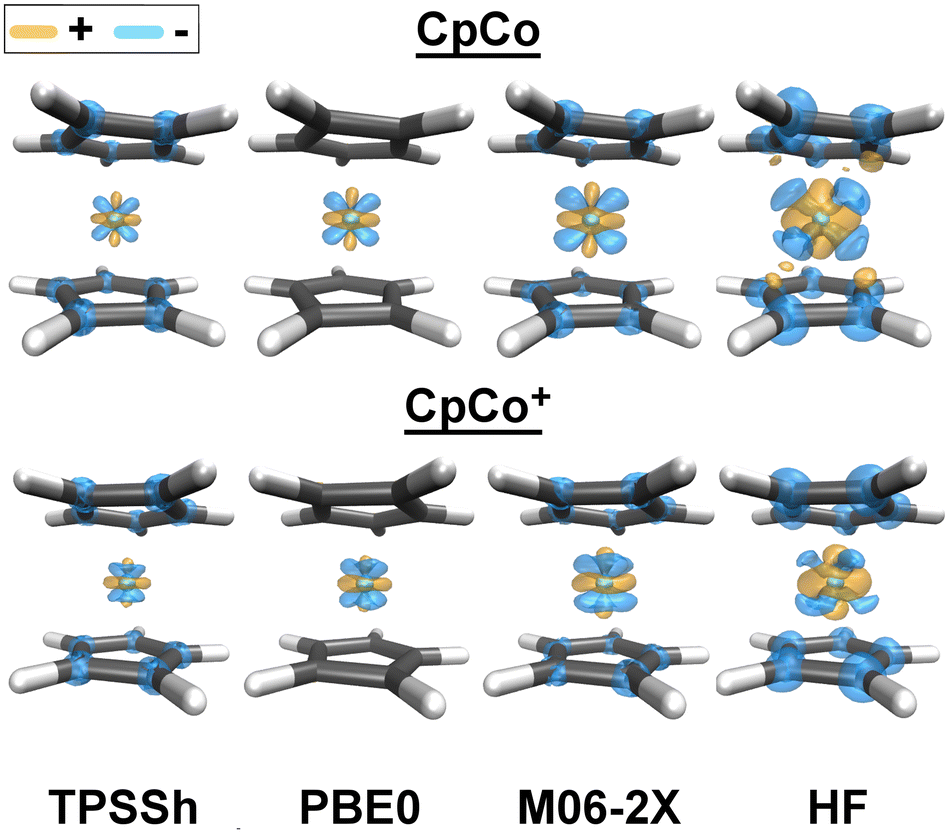
This reference orbital effect can be rationalized by the inspection of the MO diagrams of Fig. 6, where the QRO-MO energies of the orbitals used in the correlation calculations on neutral Cp₂Co are plotted. Increasing HF exchange in the density functional causes increased ligand field splitting, resulting in less delocalization of the d_z² electron into the d_xz/yz orbitals. A similar effect is observed for Cp₂Co⁺, analogous MO diagrams can be found in the ESI.†

Fig. 6 Molecular orbital diagrams of the QRO orbitals of neutral Cp₂Co from single-point calculations using various DFT methods and HF at the cc-pVTZ-DK level on the BP86-D3 optimized geometry. These are the orbitals used as references in DLPNO-CCSD(T) calculations. The method for each MO diagram is labeled on top along with the corresponding T₁ diagnostic. Selected orbitals from BP86 and HF calculations are plotted and labeled at the bottom of the figure.

The increased ligand field splitting and localization of the d_z² electron, predicted with higher HF exchange, translates to lower ionization energies in DLPNO-CCSD(T₀) calculations, as can be seen in Fig. 3. Moreover, the TPSS and TPSSh reference orbitals seem to have slightly lower electron density on the Cp rings relative to the others, and therefore, must also have higher electron density on cobalt. This results in slight lowering of the IE at both DFT and DLPNO-CCSD(T₀) levels for TPSS and TPSSh, where TPSS has lower IEs compared to GGA methods, and TPSSh predicting lower IEs than hybrids with higher fractional HF exchange at both DFT and DLPNO-CCSD(T₀) levels (Fig. 3). This is not the case for M06-2X, perhaps due to the high HF exchange and the highly parameterized nature of the functional. Nevertheless, the lower electron density on the Cp rings could not be explained based on the MO energies in Fig. 6. Finally, the HF reference leads to significantly lowered electron density on the Cp rings relative to BP86. The difference in electron density on cobalt is, however, more difficult to analyze compared to the other methods. This is due to the completely different electronic structure as seen in the HF MO diagram in Fig. 6, which also leads to vastly different orbital mixing compared to BP86.

The MO diagrams in Fig. 6 reveal stark differences in the electronic structure calculated with different methods. The (meta-) GGA methods and TPSSh have electronic structures consistent with a textbook MO diagram of a metallocene (the d-orbitals being the highest in energy). However, increasing the fractional HF exchange, results in a systematic downward shift in energy of the doubly occupied cobalt d-orbitals, until, at 50% HF exchange, they are below the π bonding orbitals of the Cp rings. This is even more pronounced for the Cp₂Co⁺ cation (see ESI†), where e₁′′ π bonding orbitals are the HOMOs for the B3LYP diagram and all methods employing higher fractional HF exchange. It should be noted that in valence photoelectron spectroscopy studies of cobaltocene and other metallocenes, the first ionization bands are confidently interpreted as ionization of electrons from metal-based orbitals. Such an interpretation appears clearly more consistent with the MO diagrams of the (meta-)GGA functionals and TPSSh but not at all with the MO diagrams of BHLYP, M06-2X and HF.⁹⁴

The electronic structure of cobaltocene according to the HF orbitals appears highly unusual, as the a₁′ (d_z²) orbital is lower in energy than the σ orbitals of the Cp rings, and is so mixed with one of them that they cannot be distinguished. Furthermore, one e₂′ (d_xy/x²−y²) and one e₁′′ orbital (Cp–Co π-bonding) have also become highly mixed, resulting in symmetry breaking of these degenerate orbitals. This seemingly exaggerated lowering of the metal d-orbitals for HF and hybrid functionals with >50% HF exchange appears to result in an overall qualitatively incorrect electronic structure, suggesting these reference orbitals to be unsuitable for CCSD(T) calculations.

The T₁ diagnostic,⁹¹ the normalized Euclidean norm of the t₁ singles vector (not to be confused with the T₁ iterative triples) is commonly used to diagnose multi-reference character of molecules. While the usefulness of the T₁ diagnostic for determining multireference character is nowadays debated, the diagnostic is arguably still useful for determining the quality of the reference orbitals in a coupled cluster calculation, seeing as it is a measure of the contribution of singles excitations to the correlation energy. Values >0.02 are traditionally regarded as suspicious, although it has been pointed out this threshold may not apply for open-shell and transition metal compounds.^24,95 The T₁ diagnostic from each DLPNO-CCSD calculation with a given set of reference orbitals is shown at the top of Fig. 6. The value of the T₁ diagnostic for the DLPNO-CCSD(HF) calculation is found to be relatively high, 0.0296, suggesting indeed the HF reference to be problematic as previously discussed. All DFT references in contrast give much lower T₁ diagnostics for Cp₂Co. Interestingly, the T₁ diagnostic decreases from 0.0176 (BP86) with increasing HF exchange with the PBE0 reference giving the lowest value (0.0087). The BHLYP and M06-2X orbitals result in slightly larger T₁ values (0.0129 and 0.0166) than PBE0, yet smaller than BP86. Thus, apart from the high T₁ value for HF, the T₁ values do not correlate well with the MO diagram analysis previously discussed; e.g. M06-2X and BHLYP orbitals might seem more plausible than BP86 orbitals based on the T₁ diagnostic, yet the MO diagrams from M06-2X and BHLYP suggest chemically implausible orbitals.

Recent studies by Pantazis and coworkers on spin-state energetics of Mn, Co and Fe complexes calculated with DLPNO-CCSD(T), also found that BP86 reference orbitals consistently gave the best results in DLPNO-CCSD(T) calculations.^76,77,96 In one study,⁷⁶ the number of calculated PNOs per electron pair were compared for different reference orbitals, with BP86 giving the highest numbers. A similar analysis was performed for cobaltocene, as shown in the ESI,† where BP86 also gave the highest numbers. In a recent study,⁷⁷ the DLPNO-error (compared to full CC) was also compared with different reference orbitals, where DFT orbitals were found to give lower DLPNO errors than HF orbitals (although PNO extrapolation considerably reduced this effect). As discussed by Pantazis and coworkers, DFT orbitals are overall likely to give more realistic orbital shapes than HF orbitals for TM compounds, which affects the domain definitions in DLPNO-CC calculations and thus influences also the DLPNO local error. The results in this work are overall more consistent with the DFT orbitals giving a more realistic description of the intrinsic electron correlation problem as seen via the MO diagrams (regardless of errors from the local approximation).

3.3 High accuracy calculations of vertical and adiabatic ionization energies of cobaltocene

In this section we detail our attempt to push the accuracy of our multi-step DLPNO-CCSD(T) protocol to the limit as we tried to reproduce the experimental ZEKE-MATI adiabatic and vertical ionization energy of cobaltocene to within chemical accuracy. The ionization energies were calculated according to eqn (4). Calculations were performed on the BP86-optimized geometries and the zero-point vibrational energy correction from BP86 was used for the adiabatic IE. All E(CCSD) and E(T₀) correlation energies are calculated using CPS(2) extrapolations as described in the computational details. The ΔE(ref.) contribution was calculated using a QRO-reference determinant of BP86 orbitals; it was not extrapolated (due to the use of non-selfconsistent HF energies; see ESI,† for a discussion) but was evaluated using the largest basis set reference energies from the CCSD(T) calculation. Both E(T₁)_corr and E(CV)_corr were evaluated at different PNO cut-offs and basis set sizes (see Table 3), and included in the IE at the highest level we could obtain. The DKH scalar relativistic Hamiltonian was used throughout and three basis set families were compared: cc-DK, def2-DKH and cc-pwCVnZ-DK(on Co)/cc-pVnZ-DK (on C,H) (labelled cc-CV/V). The importance of scalar relativity for the ionization energy was separately investigated by comparing non-relativistic, ZORA and DKH Hamiltonians at both CCSD(T) and DFT levels of theory, as shown in the ESI.† Scalar relativity was found to give a surprisingly large contribution of ∼−0.08 eV to the adiabatic ionization energy of cobaltocene, primarily resulting from the reference energy contribution.

Table 3 Convergence of ΔE(CCSD(T₀)), ΔE(T₁)_corr and ΔE(CV)_corr contributions to adiabatic- and vertical-IEs of Cp₂Co using cc-pwCVnZ (Co)/cc-pVnZ (C,H) basis sets, compared to experiment^a

	Adiabatic IE					Vertical IE
	TZ	QZ	5Z	TZ/QZb	QZ/5Z^b	TZ	QZ	5Z	TZ/QZ^b	QZ/5Z^b
a All energies are shown in eV. Correlation energies shown were extrapolated to the CPS limit except where indicated. b CBS(3/4) and CBS(4/5) extrapolations. c CBS(3/4) and CBS(4/5) extrapolations use the reference energy from the larger basis set, e.g. QZ for CBS(3/4). d Convergence of ΔE(T1)corr and ΔE(CV)corr calculated with different PNO cut-offs and basis sets. e L.PNO* refers to TCutPNO = 10^−6, with other cutoffs the same as N.PNO. f ΔE(ZPE) from harmonic frequency calculations at the BP86-D3/def2-TZVP level, included in all adiabatic IETot. g Total ionization energy where the highest-level ΔE(T1)corr and ΔE(CV)corr available, labeled with an asterisk (*) for both adiabatic and vertical IE, were added to the CCSD(T0) ionization energy of each column.
ΔE(ref.)^c	5.3009	5.2973	5.2932	5.2973	5.2932	5.4153	5.4142	5.4119	5.4142	5.4119
ΔE(CCSD)	−0.0012	0.0467	0.0508	0.0816	0.0552	0.1667	0.2263	0.2353	0.2697	0.2447
ΔE(T0)	−0.2438	−0.2357	−0.2330	−0.2298	−0.2301	−0.2616	−0.2532	−0.2516	−0.2471	−0.2499
IE CCSD(T0)	5.0559	5.1083	5.1110	5.1491	5.1183	5.3204	5.3873	5.3956	5.4368	5.4067
	ΔE(T1)corr^d
L.PNO*^e	−0.0205	−0.0171		−0.0146		−0.0232	−0.0235		−0.0197
N.PNO	−0.0198	−0.0160		−0.0133		−0.0247	−0.0250		−0.0155
T.PNO	−0.0181	−0.0149		−0.0126		−0.0258	−0.0262		−0.0153
CPS	−0.0171	−0.0139		−0.0117*		−0.0271	−0.0275		−0.0130*
	ΔE(CV)corr^d
N.PNO	−0.0072	0.0018		0.0084		0.0071	0.0183		0.0265
T.PNO	−0.0032	0.0026		0.0068		0.0166	0.0195		0.0217
CPS	−0.0037	0.0017		0.0056*		0.0158	0.0183		0.0200*
ΔE(ZPE)^f	0.1456
IETot.^g	5.1960	5.2479	5.2506	5.2887	5.2579	5.3274	5.3943	5.4026	5.4438	5.4137
Exp.	5.3275					5.4424

---

The calculated adiabatic IEs are shown in Fig. 7 (left), along with their respective errors relative to experiment. The CBS(2/3) extrapolations with cc-DK and cc-CV/V basis sets result give very small errors of 10 meV w.r.t. experiment; but this is found to be due to error cancellations as the IE is overestimated with respect to the largest extrapolated value, CBS(4/5). The DKH-def2 CBS(2/3) extrapolation is unusually bad. In CBS(3/4) extrapolations, however, all basis set families perform similarly, where the CBS errors at the T₀ level range from −33 to −40 meV, which are slightly higher than previously observed with N.PNO cut-offs (Fig. 2). Adding the ΔE(T₁) correction (ΔE(T₁)^CPS/CBS(3/4)_corr) lowers the IE by 7 meV for def2 basis sets and 12 meV for the others, increasing the error to −52 meV for cc-pV(T/Q)Z-DK, −44 meV for the other basis sets. The largest extrapolation, CBS(4/5), increases the error even further for the cc-CV/V basis sets, or to −75 meV at the (T₁) level. The CBS(3/4) and CBS(4/5) extrapolations are much more consistent using cc-pVnZ-DK basis sets for all atoms, with errors of −52 and −55 meV, respectively, at the T₁ level and converge to a slightly higher and more accurate adiabatic IE than the cc-CV/V basis set combination.

Fig. 7 Adiabatic- (left) and vertical- (right) ionization energies of Cp₂Co calculated with DLPNO-CCSD(T₀) using 3 basis set families, cc-pVnZ-DK (blue), cc-pwCVnZ-DK(Co)/cc-pVnZ-DK(C,H) (red) and DKH-def2-NZ (green). The IE is plotted as a function of basis set cardinal numbers with CPS extrapolation always included at the DLPNO-CCSD(T₀) level. The squares represent IEs from two-point CBS extrapolations from the curve, placed between the respective basis sets on the x-axis. The values labelled with crosses include additional ΔE(T₁) corrections (calculated at the CBS(3/4) level with CPS extrapolation). All values include BP86-D3 ZPE corrections. The experimental IEs are shown with a dashed line.

The right side of Fig. 7 shows the calculated vertical IE. Again, the def2 basis sets have much larger errors in CBS(2/3) extrapolations but perform similarly to the others in CBS(3/4) extrapolations, in which the DKH-def2 error is −11 meV, whereas the cc-CV/V basis set combination has an error of −6 meV, and cc-pVnZ-DK for all atoms 1 meV at the (T₀) level. Analogous to the adiabatic IE, the E(T₁) correction always increases the errors by lowering the IE, this time by 13 meV for all basis sets. Also conforming to the adiabatic case, the error for the cc-CV/V basis sets is increased in the CBS(4/5) extrapolation to −36 meV at the T₀ level and −49 meV at the T₁ level. This was also observed for cc-pVnZ-DK basis sets on all atoms, although to a lesser extent, leading to a final error of −28 meV in vertical IE when applying the E(T₁) correction to the CBS(4/5) vertical IE.

The larger-basis cc-CV/V family values are collected in Table 3 and decomposed into ΔE(ref.), ΔE(CCSD), ΔE(T₀), ΔE(T₁) and ΔE(CV) contributions to the adiabatic and vertical IE, with different basis sets and extrapolated values. As Table 3 shows, ΔE(CCSD) is an order of magnitude smaller than the ΔE(T₀) contribution in the adiabatic case, whereas the vertical ΔE(CCSD) and ΔE(T₀) are of similar size with opposite signs, converging towards a combined correlation contribution close to 0 in their contribution to the vertical IE. In both cases, the ΔE(CCSD) contribution is quite far from convergence at the TZ level, but nearly converged at the QZ level, causing an overestimate in the CBS(3/4) extrapolation relative to CBS(4/5). On the other hand, CBS extrapolations of ΔE(T₀) contributions are much more consistent. The ΔE(T₁) and ΔE(CV) corrections have opposite signs in adiabatic- and vertical-IE contributions (when converged), with ΔE(T₁) being twice as large in the adiabatic case, leading to lowering of the DLPNO-CCSD(T₀) IE, and thereby resulting in larger errors. The opposite is true for vertical IEs, however, where ΔE(CV)_corr is larger, and the DLPNO-CCSD(T₀) error is decreased.

As the ΔE(CV) and ΔE(T₁) corrections can be quite computationally expensive, their convergence with respect to basis set size were analyzed in order to determine the lowest level of theory at which reasonable accuracy is retained. The lower part of Table 3 shows the contribution of the ΔE(T₁) and ΔE(CV) correction to the adiabatic and vertical IE with increasing size of the cc-CV/V basis sets at different PNO cut-offs. The ΔE(T₁) correction is found to be very similar for both adiabatic- and vertical-IEs, −12 to −13 meV at the highest level calculated(CPS/CBS(3/4)). The ΔE(T₁) correction is not very sensitive to the PNO cutoffs or basis set size. For example the difference between L.PNO and CPS energies in CBS(3/4) extrapolations for adiabatic- and vertical-IEs are only 3 and 6 meV, respectively. This suggests that the correction can be calculated with a small PNO cutoff or a small basis set with minimal loss in accuracy. This has considerable implications for the computational cost as the ΔE(T₁) correction will dominate the cost of these calculations if performed with large basis sets and tight PNO cutoffs. However, it should be noted that ΔE(T₁) is small in magnitude for this particular molecule and property and the convergence of the ΔE(T₁) correction is likely somewhat system- and property dependent (see 3.4 and ESI†).

The ΔE(CV) correction to the adiabatic IE is found to be around 6 meV at the highest level calculated. The convergence is very similar between different PNO cut-offs, with only a 2 meV difference between N.PNO and CPS, the latter requiring much more computational effort. This is likely a result of the T_CutPNO scaling factor (0.01) used by default when core electrons are correlated in ORCA. Including a ΔE(T₁)^CBS(3/4)_N.PNO correction in both frozen-core and all-electron calculations only contributes 0.1 meV to ΔE(CV)_corr, suggesting that ΔE(T₁) is not important for correlation of core electrons up to 2s/2p of cobalt or the 1s of carbon. However, in calculations where we tested a more conventional frozen core approximation with 3s and 3p of cobalt also frozen, inclusion of ΔE(T₁) was important in calculations of ΔE(CV)_corr (see ESI†). For the vertical IE, the ΔE(CV) correction is curiously larger, or 20 meV in CBS(3/4) calculations with CPS energies. As in the adiabatic case, including a ΔE(T₁)^{N.PNO/CBS(3/4)}_corr correction in AE and FC calculations has no contribution to ΔE(CV)_corr. Because the ΔE(CV) correction is so far from convergence at the TZ level with N.PNO cut-offs, the CBS(3/4) extrapolation is a bit overestimated. Both T.PNO and CPS cut-offs, however, are quite well converged already at the TZ level.

After careful consideration of the basis set convergence of all of the different contributions to the correlation energy of the IE of cobaltocene, we can compare the combined best estimates of all terms in eqn (4) to the high-resolution experimental value. Chemical accuracy (1 kcal mol⁻¹ = 0.04 eV) appears to be reached for the vertical ionization energy of cobaltocene with the prediction of 5.41 eV, giving an error of 0.03 eV compared to experimental value of 5.4424 ± 0.0006. The calculated adiabatic ionization energy is 5.26 eV which is off by 0.07 eV compared to the experimental value of 5.3275 ± 0.0006 eV. It should be noted here that the high accuracy of the ZEKE-MATI experiments does not necessarily translate to the same accuracy of the vertical IE as the adiabatic IE, as the experimental vertical IE corresponds to the most intense vibronic peak measured which is not the exact same quantity as the calculated vertical IE. A recent study estimated the difference to be on the order of 0.05–0.1 eV for metallocene spin-crossover energies, including for Cp₂Co⁺.⁷⁹ A more detailed comparison would consider a simulation of the vibronic spectrum which was not performed here.

It is possible that the remaining error in the adiabatic IE stems from the DFT-calculated ZPE (ZPE being larger in magnitude than many of the correlation energy contributions), however, we note that the ZPE varies very little with different density functionals (see ESI†). An exploration of an anharmonic contribution to the ZPE is beyond the scope of this work. A contribution from higher order coupled cluster terms (e.g. full CCSDT) is also a possibility, which is also outside the scope of this study and likely unfeasible. Finally, a spin-orbit coupling contribution to the ionization energy is yet another possibility. Overall, the results are highly satisfactory, suggesting that close to chemical accuracy is achievable for the gas phase redox properties of organometallic redox agents with CCSD(T).

3.4 Ionization energies of first-row metallocenes

A high-accuracy ZEKE-MATI determination is unfortunately only available for cobaltocene and no other unsubstituted metallocenes. However, ionization energy determinations of other metallocenes are available from electron-transfer equilibrium experiments using Fourier transform ion cyclotron resonance mass spectrometry.^30,31 The experimental values were determined at 350 K, with uncertainties of ±1.5 kcal mol⁻¹ (±65 meV), i.e. 2 orders of magnitude larger than in the ZEKE-MATI experiments.³² As these IE values are from 350 K equilibrium experiments (i.e. free energy differences) instead of 0 K threshold ionizations, thermal- and entropic-corrections need to be considered.

Based on the calculations for cobaltocene in the previous section, two protocols were tested balancing computational cost while hopefully maintaining accuracy. The IEs were calculated with eqn (5) and (6) in protocols (1) and (2), respectively. The cc-pVnZ-DK basis set family with the DKH Hamiltonian was used. The E(ref.) energies came from the larger cc-pVQZ-DK calculation in the CBS(3/4) correlation extrapolations. A ΔG_corr term including thermal and entropic contributions at 350 K is now included instead of just ΔE(ZPE).

The first protocol, using CPS(2) energies in CBS(3/4) extrapolations, including a N.PNO CBS(3/4) ΔE(T₁) correction, is quite costly and could easily be prohibitive for larger systems. We therefore tested another protocol (2) using the more economical CPS(1) energies in M-CBS(3/4) extrapolations, where the cc-pVTZ-DK basis set is kept fixed for C and H atoms, only changing the basis set of the metal atom (cc-pV(T/Q)Z-DK). As shown in the previous section not much is gained from CPS extrapolations of the E(T₁)_corr correction, especially considering the extreme computational cost. The convergence of E(T₁)_corr was analyzed separately for ferrocene, as the correction is an order of magnitude larger than for cobaltocene (0.25 eV vs. −0.01 eV). The correction converges fairly reliably and can be computed efficiently with a small basis set and a small PNO cutoff. Here the correction was calculated by M-CBS(3/4) extrapolations using N.PNO for all cut-offs except T_CutPNO = 10⁻⁶, by simply calculating the larger PNO cut-off in the CPS⁽¹⁾ extrapolations at the T₁ level, by which one obtains both E(T₀) and E(T₁) energies, which can then be used for M-CBS(3/4) extrapolations. In this manner, all terms for the IE apart from ΔG_corr can be obtained in four calculations of each species, neutral and cation. This protocol is a slightly modified version of a protocol suggested by Drosou et al. for spin-state energies,^76,77 with the main difference being the use of a E(T₁)_corr additive term instead of using costly DLPNO-CCSD(T₁) calculations throughout.

The ΔE(CV) correction was not included in either protocol, as the correction was negligible for the adiabatic IE of Cp₂Co and unlike the ΔE(T₁)_corr, was not expected to be generally important (see Table 3). The most important core–valence effect likely comes from correlating the 3s and 3p shell of the metal ion, shells that are already correlated in the frozen-core definition used in this work. See ESI,† for a discussion.

All metallocenes, except neutral sextet Cp₂Mn, are in an eclipsed conformation. All optimizations were first carried out with BP86 using def2-TZVP bases sets and the D3 dispersion correction, which performed best in Section 3.2.1. However, the BP86-D3 geometry of sextet Cp₂Mn was found to be quite distorted, where half of each Cp ring was pushed towards the Mn ion (see geometries in ESI†). This effect is unlikely to be physical as no JT-distortion is expected for the d⁵ system in a ⁶A_1g state. Relativistic methods, integral treatment, integration grids and dispersion correction were all tested as a potential source of the error, but could all be excluded. Functionals with fractional HF exchange up to 25% from Section 3.2.1, were tested and, thereof, PBE0-D3 had the least distorted geometry, although not a perfect D_5h symmetry. Combining PBE0 with the modern D4 dispersion correction appears to fix the issue, resulting in D_5h symmetry.⁴⁶ As the BP86-D3 Cp₂Mn (⁶A₁′) geometry was considered unreliable, geometries of all metallocenes were also optimized with PBE0 at the same level, with the exception of D4 dispersion for Cp₂Mn. The DLPNO-CCSD(T₀/T₁) calculations were then carried out on BP86-D3 geometries with BP86 reference orbitals, and PBE0-D3/D4 geometries with PBE0 reference orbitals. This allowed for comparison of the two across the metallocene series. A distorted BP86-D3 geometry of ⁶A₁′ Cp₂Mn was previously reported by Radon and coworkers,⁷⁹ who suggested self-interaction in BP86 as a cause, yet, others appear not to have encountered this issue.^29,76,80

The M–C and C–C distances from BP86-D3 and PBE0-D3 geometries are compared to experimental values from GED experiments in Table 4.^97–100 Cp₂Co was omitted as its geometry was discussed in details in section 3.2.1. Both methods predict very similar metal–carbon (M–C) distances, which are generally within 1 pm of the experimental value with the exception of Cp₂Fe where the deviations are 1.9 and 2.2 pm for BP86-D3 and PBE0-D3, respectively. Moreover, PBE0-D3 systematically underestimates the C–C bond length by 1.5–2 pm, whereas BP86-D3 geometries are consistently within 1 pm of the GED value. We note, however, that the GED geometries were not corrected for thermal motion. Assuming the other metallocenes behave similarly to Cp₂Fe, the equilibrium M–C distance may be approximately 1 pm shorter than the experimental GED value.^79,83

Table 4 Interatomic distances in optimized DFT-D3/D4 structures with def2-TZVP basis sets compared to GED experiments^a

	Cp2V	Cp2Cr	Cp2Mn^b	Cp2Fe	Cp2Ni
	^4A2′	^3A1′	^6A1g	^1A1′	^3A2′
a All distances in pm. Geometries were not corrected for thermal motion. The geometry of Cp2Co is omitted as it was discussed in detail in Section 3.2.1. All geometry optimizations were performed with D3 dispersion, apart from Cp2Mn. b PBE0 geometries of Cp2Mn calculated with D4 dispersion to remove distortion (see text). c Ref. 97–100.
	M–C
BP86	227.0	216.3	—	204.5	219.3
PBE0	227.3	216.2	238.8	204.2	219.3
Expt.^c	228.0	216.9	238.0	206.4	219.6
	C–C
BP86	142.7	143.3	—	143.4	142.9
PBE0	141.5	142.0	141.5	142.0	141.6
Expt.^c	143.4	143.1	142.9	143.5	143.0

---

Friesner and coworkers produced impressive results of this test set of metallocenes, using their AFQMC method and compared the results to DLPNO-CCSD(T₀)-CBS(3/4) calculations using B3LYP geometries and reference orbitals.²⁹ They concluded that the DLPNO-CCSD(T₀) calculations were no more reliable than DFT, and questioned whether this was due to inherit shortcomings of the coupled cluster method, or caused by the approximations in the DLPNO treatment. Although they did show that errors of Cp₂Mn could be reduced using tighter PNO cut-offs and (T₁) triples, this was not the focus of their study and further analysis was suggested. Taking these considerations into account, the two protocols described at the beginning of the section were used to calculate the adiabatic IEs of the first row metallocene series with both BP86-D3 geometries and reference orbitals (protocol (1)), and PBE0-D3/D4 geometries and reference orbitals (protocols (1) and (2)). The results were compared to the calculations of Friesner and coworkers and the ion cyclotron experiments of Richardson and coworkers.^29–31 We note that the experimental IE of Cp₂Co in this section refers to the same 350 K free energy of ionization from the ion cyclotron experiments. The results are shown in Table 5.

Table 5 Adiabatic IEs of first row metallocenes calculated with DLPNO-CCSD(T₀/T₁) with N.PNO and CPS cut-offs in CBS(3/4) extrapolations (cc-pVnZ-DK). Results are compared to experimental data at 350 K and calculations from literature^a

	Expt.^c	This work					Friesner et al.^b
		N.PNO	N.PNO	CPS	CPS	CPS	N.PNO	AFQMC
		CCSD(T0)	CCSD(T1)	CCSD(T0/T1)(1)	CCSD(T0/T1)(2)	CCSD(T0/T1)(1)	CCSD(T0)
		PBE0 ref.^d	PBE0 ref.^d	PBE0 ref.^e	PBE0 ref.^f	BP86 ref.^e	B3LYP ref.
a All energies are reported in eV. b From ref. 29. c From ref. 30 and 31. Reported experimental uncertainty was ±0.065 eV. d DLPNO-CCSD(T0/T1) calculations, CBS(3/4) energies with N.PNO cut-offs. e Protocol (1): CPS(2) energies in CBS(3/4) extrapolations, using a ΔE(T1) correction from the N.PNO-CBS(3/4) calculations. f Protocol (2): CPS(1) energies with M-CBS(3/4) extrapolations and ΔE(T1) correction from M-CBS(3/4) calculations with TCutPNO = 10^−6. g Cp2Mn geometries use D4 instead of D3 dispersion to avoid distorted geometries (see text above). h Mean unsigned error (MUE), mean signed error (MSE) and maximum unsigned error (|Max E|).
Cp2V	6.700	6.705	6.648	6.600	6.550	6.541	6.994	6.665
Cp2Cr	5.529	5.300	5.437	5.536	5.370	5.585	5.369	5.688
Cp2Mn^g	6.179	6.640	6.438	6.257	6.208	6.247	6.658	6.335
Cp2Fe	6.639	6.582	6.772	6.811	6.669	6.876	6.773	6.625
Cp2Co	5.355	5.340	5.303	5.313	5.216	5.358	5.308	5.392
Cp2Ni	6.236	6.377	6.279	6.243	6.172	6.299	6.393	6.255
MUE^h		0.152	0.105	0.063	0.095	0.098	0.212	0.070
MSE		0.051	0.040	0.020	-0.075	0.045	0.143	0.054
|Max E|		0.461	0.259	0.172	0.159	0.237	0.478	0.160

---

Overall, the DLPNO-CCSD(T₀/T₁) protocol (1) using PBE0 reference orbitals performed best of the methods tested here, with a mean unsigned error (MUE) of 0.063 eV, which is very close to the experimental uncertainty (±0.065 eV) and a MaxError of 0.172 eV. These errors can be compared to values in the first and second column of the table where CPS extrapolation and ΔE(T₁) correction contributions were not included; giving MUE of 0.152 eV and a Max Error of 0.461 eV (if CPS extrapolation and ΔE(T₁) contributions are excluded) or a MUE of 0.105 eV and a Max Error of 0.259 eV (if CPS extrapolation is excluded). This demonstrates both the importance of reducing PNO errors and to account for the effect of iterative triples for a robust DLPNO-CCSD(T)-based protocol.

The values for protocol (1) follow the same trend when BP86 reference orbitals are used, however, the errors are generally slightly larger, leading to a MUE of 0.098 eV. This contrasts the results for cobaltocene in the previous section, suggesting that PBE0 may provide a better description of the electronic structure of the other metallocenes. In both cases, the largest outlier is Cp₂Fe with errors of 0.237 and 0.172 eV for BP86 and PBE0 reference orbitals, respectively. Interestingly, this is the only complex whose M–C distance had deviations over 1 pm from the GED experiments. Turning off D3 dispersion lowers the deviation of M–C distance from 1.9 to 1.4 pm for BP86, but does not significantly affect the DLPNO-CCSD(T₀/T₁) results (not shown). The ΔE(CV) correction was also tested as the source of the error in IE for Cp₂Fe, resulting in only a 10 meV shift of the IE in the wrong direction. In the case of Cp₂Mn, however, the better geometry (PBE0-D4) reduced the error in IE from 0.164 to 0.078 eV, largely due to the ΔG_corr contribution. Notwithstanding, protocol (1) using PBE0 orbitals performs very similarly to the AFQMC method used by Friesner and coworkers with respect to both MUE and |Max| error.

Protocol (2) was only tested using PBE0-D3/D4 geometries and reference orbitals, as PBE0 performed better overall and did not suffer from the previously discussed issue of distorted geometry for ⁶A_1g Cp₂Mn. This protocol does not appear to be converged with respect to the CCSD(T₀) contribution to the adiabatic IE, as it systematically underestimated the IEs compared to protocol (1) with PBE0-D3/D4 geometry and reference orbitals. This is likely, in part, due to over-stabilization of high spin species when the method is far from convergence in terms of captured correlation energy. The worst cases are underestimations by 0.166 and 0.142 eV in the adiabatic IEs of Cp₂Cr and Cp₂Fe compared to protocol (1), where the spin is increased after ionization, thus over-stabilizing the cation. The mildest cases, on the other hand, are Cp₂V and Cp₂Mn, whose IEs are both underestimated by 0.049 eV, as both neutral molecules are high spin and their spin is lowered upon ionization. The source of the error is further discussed below in relation to Fig. 8, where different contributions to the error of both protocols are compared. Notwithstanding, the MUE is only increased to 0.095 eV, which is comparable to protocol (1) using BP86-D3 geometries and reference orbitals. Although |MaxE| is reduced, this is due to fortunate error cancellation involving Cp₂Fe, which results in Cp₂Co having the largest error for this protocol.

Fig. 8 Errors in adiabatic ionization energies of the metallocenes relative to experimental values from ref. 30 and 31, calculated with protocol (1) using BP86-D3 geometries and reference orbitals (blue) and PBE0-D3/D4 geometries and reference orbitals (red), and protocol (2) with PBE0-D3/D4 geometries and reference orbitals (green). Each line from left to right shows the error at the CCSD(T₀) level (square), error after adding the E(T₁)_corr correction (diamond), and the final error after adding ΔG_corr (filled circle) or ΔH_corr (empty circle). ΔG_corr is the ZPE including thermal and entropic corrections at 350 K from harmonic frequency calculations, whereas ΔH_corr only includes the thermal corrections, omitting entropy terms.

Fig. 8 compares the errors of both protocols at the CCSD(T₀) and CCSD(T₀/T₁) (after adding (ΔE(T₁)_corr)). Furthermore, adding only thermal corrections (ΔH_corr), and both thermal- and entropic corrections (ΔG_corr), to the E(ZPE) term is compared. Non-rigid molecules tend to have low frequency large amplitude motions (LAMs), which are anharmonic in nature and may be poorly described by the RRHO approximation. They mostly affect the calculated vibrational entropy.¹⁰¹ In cases where there is significant difference between ΔG_corr and ΔH_corr, the former was, however, in general closer to experiment with the exception of Cp₂Mn. The ΔE(T₁) correction is required for accurate IEs of Cp₂Cr, Cp₂Mn and Cp₂Ni, whereas it appears to reduce agreement with experiment for Cp₂V and Cp₂Fe, especially Cp₂Fe. The ΔE(T₁) correction was analyzed separately for Cp₂Fe and found to be reliably converged (see ESI†). Protocol (2) predicts lower IEs in all cases, compared to protocol (1) with the same geometry and reference orbitals (green and red, Fig. 8). This difference is mainly at the ΔE(CCSD(T₀)) level, as the ΔE(T₁) correction is very close with the largest difference being 0.02 eV for Cp₂Cr, indicating that calculating ΔE(T₁)_corr in CBS(3/4) extrapolations with T_CutPNO = 10⁻⁶, and “NormalPNO” settings for all other cut-offs in the DLPNO method is a good approximation. This is fortunate as it greatly reduces computational costs. Protocol (2) approximates the ΔE(CCSD(T₀)) energy of protocol (1) both the CPS extrapolation, and the CBS extrapolation. Although not shown in the figure, the CPS(1) extrapolation, using T_CutPNO = 10⁻⁶/3.33 × 10⁻⁷ with “NormalPNO” for other cut-offs, compared to 10⁻⁶/10⁻⁷ and “TightPNO” for other cut-offs in protocol (1), is generally a good approximation with the largest deviation being −0.05 eV for Cp₂Mn, but generally 0.005–0.01 eV for the other metallocenes. The other approximation, M-CBS(3/4), where only the metal basis set size was increased in the CBS extrapolations, resulted in deviations of −0.04 to −0.06 eV in IE at the cc-pVQZ-DK (metal only) level for all metallocenes, causing even larger errors in the CBS extrapolation. Although the oxidation is mostly metal based, removing an electron has an effect on the covalent ligands, especially ligands like Cp rings with a cyclic aromatic π system. For more conventional coordination complexes, this could perhaps be somewhat alleviated by increasing the basis set size of the metal and directly coordinated atoms, as opposed to only the metal atom, in CBS extrapolations. In the case of metallocenes, however, this would mean including all 10 carbon atoms, which would be very similar to the CBS extrapolation of protocol (1).

4 Conclusions

The ionization energies of the metallocene redox agents pose an interesting challenge for both density functional theory approximations as well as modern wavefunction theory. Cobaltocene is the only metallocene that has been measured in a high-resolution ZEKE-MATI gas phase experiment, with an uncertainty of only ±0.0006 eV.³² This makes the molecule highly suitable to testing the capability of state-of-the-art coupled cluster theory using local correlation approximations. In this work we systematically tested a DLPNO-CCSD(T)-based protocol, with respect to practically all of the important variables that enter into such calculations.

Geometries of neutral cobaltocene were found to be well described at both the BP86 and PBE0 level based on a comparison to an experimental structure from gas phase electron diffraction.⁸¹ Differences between the functionals were found for Co–C distances in the Cp₂Co⁺ cation (where experimental data is unfortunately lacking). Special attention was paid to the influence of the orbitals in the reference determinant in the DLPNO-CCSD(T) and we tested using orbitals from both the HF method and several different density functionals. The singles-based T₁ diagnostic was found not to be helpful in distinguishing reference orbitals at the DFT level. Interestingly, the HF determinant was found to be an exceptionally bad reference in the DLPNO-CCSD(T₀) calculations. The closed-shell SCF solution of Cp₂Co⁺ was unstable at the HF level, and a stable UHF solution turned out to be a flawed symmetry-broken spin-coupled solution. Analysis of MO energies of the Cp₂Co QRO orbitals, used as references in the correlation calculations, (Fig. 6) revealed that increasing the HF exchange leads to larger ligand-field splitting due to lowering the energy of the non-bonding Co d orbitals, which start to overlap with occupied Cp π orbitals for B3LYP (20% HF exchange), and with high HF exchange the Cp π orbitals become the highest doubly occupied MOs. For the HF determinant, the a₁′ (d_z²) orbital is below the Cp σ orbitals in energy. These different MO diagrams indicate considerably different orbital mixing effects which affects the CCSD electronic structure, as seen by the difference in unrelaxed DLPNO-CCSD electron density of hybrid functionals compared to BP86. The electronic structure predicted by (meta-)GGA functionals appear to be much more consistent with results from valence photoelectron spectroscopy experiments and we argue are thus more likely to form a more useful set of reference orbitals for coupled cluster calculations.⁹⁴ However, this aspect unfortunately demonstrates that coupled cluster calculations on transition metal complexes is not as black-box as would be desired, as the orbital choice is not easily known beforehand.

The error of the DLPNO approximation was systematically tested with respect to both PNO cutoffs as well as the accuracy of the perturbative triples excitations within the framework. Extrapolation of correlation energies to the complete PNO space limit, as recently suggested by Bistoni and coworkers,⁷⁴ turns out to be highly useful. The basis set convergence of calculated vertical- and adiabatic IEs of Cp₂Co was explored at the DLPNO-CCSD(T₀) level with cc-pwCVnZ-DK(Co)/cc-pVnZ-DK(C,H) (cc-CV/V), cc-pVnZ-DK and DKH-def2-NZVPP basis sets, with PNO extrapolation to the CPS limit performed for each calculation. A similar basis set limit is reached with CBS(3/4) extrapolations, however, with some differences seen with CBS(4/5) extrapolations when using the larger cc-CV/V family. The effect of the iterative triples T₁ in DLPNO-CCSD(T₁) turns out not to play a large role for the ionization energy of cobaltocene (but was found to be more important for other metallocenes). In this work we suggest the T₁ triples to be included in the form of a correction (instead of being always included) as otherwise the calculations are prohibitively expensive. The correction is found to be only loosely dependent on T_CutPNO cut-offs, and can be calculated using a small T_CutPNO = 10⁻⁶ with other cut-offs set to “NormalPNO” defaults in ORCA and either as a single-step correction using a small basis set or extrapolated to the CBS limit.

The most accurate DLPNO-CCSD(T) protocol in this work utilized CBS(4/5) basis set extrapolation of CCSD and T₀ correlation energies, with PNO-extrapolation to the CPS limit for each correlation energy, the iterative triples T₁ contribution calculated as a correction with a smaller PNO cutoff, and a core–valence correlation correction. Combined with the SCF reference energy (with BP86 orbitals) and ZPVE correction, a final adiabatic ionization energy of 5.258 eV was predicted in very good agreement with the 5.328 eV from experiment. Even better agreement was found for the vertical ionization energy, 5.414 eV vs. 5.442 eV. Scalar relativity was found to have a non-negligible effect (−0.08 eV) on the cobaltocene ionization energy and was included in all calculations.

Free energies of ionization of a series of first-row metallocenes were calculated and compared to experimental data (at T = 350 K) from ion cyclotron experiments.^30,31 DLPNO-CCSD(T) protocols utilizing basis set CBS extrapolations, CPS extrapolations and a T₁ correction, based on the cobaltocene analysis, were tested on the full test test. Both BP86 and PBE0 functionals were tested as choices for geometries and reference orbitals. The results reveal that CCSD(T) appears to be fully capable of describing the ionization energies of these systems well, with the T₁ correction and the CPS extrapolation turning out to be much more important for these systems than cobaltocene. The lack of these two factors mostly explain the unsatisfactory DLPNO-CCSD(T) results obtained by Friesner and coworkers.²⁹ DLPNO-CCSD(T) calculations that account for PNO extrapolation as well as iterative triples effects give results in equally good agreement as the AFQMC results with mean unsigned errors close to the experimental uncertainty. The individual results for the test set, however, reveal a dependence on reference orbitals (BP86 vs. PBE0), perhaps due to the known varying degrees of metal–ligand covalency across the metallocene series.¹⁰² Overall, the results for both cobaltocene and the test set of metallocenes are a promising step towards the goal of a coupled cluster protocol capable of predicting redox reaction energies of real-world open-shell transition metal complexes with chemical accuracy. It is clear though that a better understanding on how to choose the orbitals for the reference determinant in coupled cluster calculations is needed. Vibrational corrections are another source of uncertainty. Our DLPNO-CCSD(T) workflow that conveniently combines basis set extrapolation, PNO extrapolation, T₁ correction and optional core–valence correction can conveniently be carried out automatically in the open-source Python-based program ASH (with an interface to ORCA).³⁵

Conflicts of interest

There are no conflicts of interest to declare.

Acknowledgements

Calculations were performed on Garpur cluster, provided by the High Performance Computing Centre from the University of Iceland. RB acknowledges support from the Icelandic Research Fund, grant No. 162880051.

References

1. T. Kealy and P. Pauson, Nature, 1951, 168, 1039–1040.
2. D. R. Van Staveren and N. Metzler-Nolte, Chem. Rev., 2004, 104, 5931–5986.
3. R. R. Gagne, C. A. Koval and G. C. Lisensky, Inorg. Chem., 1980, 19, 2854–2855.
4. W. Kaminsky, Catal. Today, 2000, 62, 23–34.
5. D. V. Yandulov and R. R. Schrock, Science, 2003, 301, 76–78.
6. S. Kuriyama, K. Arashiba, K. Nakajima, H. Tanaka, K. Yoshizawa and Y. Nishibayashi, Chem. Sci., 2015, 6, 3940–3951.
7. N. Stucke, T. Weyrich, M. Pfeil, K. Grund, A. Kindjajev and F. Tuczek, Nitrogen Fixation, 2017, 113–152.
8. M. J. Chalkley, T. J. Del Castillo, B. D. Matson, J. P. Roddy and J. C. Peters, ACS Cent. Sci., 2017, 3, 217–223.
9. M. J. Chalkley, P. H. Oyala and J. C. Peters, J. Am. Chem. Soc., 2019, 141, 4721–4729.
10. M. J. Chalkley, T. J. Del Castillo, B. D. Matson and J. C. Peters, J. Am. Chem. Soc., 2018, 140, 6122–6129.
11. R. Cai, R. D. Milton, S. Abdellaoui, T. Park, J. Patel, B. Alkotaini and S. D. Minteer, J. Am. Chem. Soc., 2018, 140, 5041–5044.
12. M. J. Chalkley, P. Garrido-Barros and J. C. Peters, Science, 2020, 369, 850–854.
13. J. Derosa, P. Garrido-Barros and J. C. Peters, J. Am. Chem. Soc., 2021, 143, 9303–9307.
14. P. Garrid-Barros, J. Derosa, M. J. Chalkley and J. C. Peters, Nature, 2022, 609, 71–76.
15. M. Pitoňák, P. Neogrády, J. Černý, S. Grimme and P. Hobza, ChemPhysChem, 2009, 10, 282–289.
16. J. Rezac, K. E. Riley and P. Hobza, J. Chem. Theory Comput., 2012, 8, 4285–4292.
17. E. F. Valeev and T. Daniel Crawford, J. Chem. Phys., 2008, 128, 244113.
18. F. Neese, A. Hansen and D. G. Liakos, J. Chem. Phys., 2009, 131, 064103.
19. C. Riplinger, B. Sandhoefer, A. Hansen and F. Neese, J. Chem. Phys., 2013, 139, 134101.
20. M. Saitow, U. Becker, C. Riplinger, E. F. Valeev and F. Neese, J. Chem. Phys., 2017, 146, 164105.
21. F. Pavošević, C. Peng, P. Pinski, C. Riplinger, F. Neese and E. F. Valeev, J. Chem. Phys., 2017, 146, 174108.
22. Y. Guo, C. Riplinger, D. G. Liakos, U. Becker, M. Saitow and F. Neese, J. Chem. Phys., 2020, 152, 024116.
23. Y. Guo, C. Riplinger, U. Becker, D. G. Liakos, Y. Minenkov, L. Cavallo and F. Neese, J. Chem. Phys., 2018, 148, 011101.
24. X. Xu, W. Zhang, M. Tang and D. G. Truhlar, J. Chem. Theory Comput., 2015, 11, 2036–2052.
25. J. Shee, B. Rudshteyn, E. J. Arthur, S. Zhang, D. R. Reichman and R. A. Friesner, J. Chem. Theory Comput., 2019, 15, 2346–2358.
26. Y. A. Aoto, A. P. de Lima Batista, A. Kohn and A. G. de Oliveira-Filho, J. Chem. Theory Comput., 2017, 13, 5291–5316.
27. Z. Fang, M. Vasiliu, K. A. Peterson and D. A. Dixon, J. Chem. Theory Comput., 2017, 13, 1057–1066.
28. Z. Fang, Z. Lee, K. A. Peterson and D. A. Dixon, J. Chem. Theory Comput., 2016, 12, 3583–3592.
29. B. Rudshteyn, J. L. Weber, D. Coskun, P. A. Devlaminck, S. Zhang, D. R. Reichman, J. Shee and R. A. Friesner, J. Chem. Theory Comput., 2022, 18, 2845–2862.
30. M. F. Ryan, J. R. Eyler and D. E. Richardson, J. Am. Chem. Soc., 1992, 114, 8611–8619.
31. M. F. Ryan, D. E. Richardson, D. L. Lichtenberger and N. E. Gruhn, Organometallics, 1994, 13, 1190–1199.
32. S. Y. Ketkov and H. L. Selzle, Angew. Chem., Int. Ed., 2012, 51, 11527–11530.
33. F. Neese, F. Wennmohs, U. Becker and C. Riplinger, J. Chem. Phys., 2020, 152, 224108.
34. F. Neese, Wiley Interdiscip. Rev.: Comput. Mol. Sci., 2022, 12, e1606.
35. R. Bjornsson, ASH – a multiscale modelling program, 2022, Version 0.9, https://ash.readthedocs.io/en/latest/.
36. J. P. Perdew, J. Tao, V. N. Staroverov and G. E. Scuseria, J. Chem. Phys., 2004, 120, 6898–6911.
37. J. W. Furness, A. D. Kaplan, J. Ning, J. P. Perdew and J. Sun, J. Phys. Chem. Lett., 2020, 11, 8208–8215.
38. J. Tao, J. P. Perdew, V. N. Staroverov and G. E. Scuseria, Phys. Rev. Lett., 2003, 91, 146401.
39. Y. Zhao and D. G. Truhlar, Theor. Chem. Acc., 2008, 120, 215–241.
40. P. J. Stephens, F. J. Devlin, C. F. Chabalowski and M. J. Frisch, J. Phys. Chem., 1994, 98, 11623–11627.
41. A. D. Becke, J. Chem. Phys., 1993, 98, 1372–1377.
42. C. Adamo and V. Barone, J. Chem. Phys., 1999, 110, 6158–6170.
43. S. Grimme, J. Antony, S. Ehrlich and H. Krieg, J. Chem. Phys., 2010, 132, 154104.
44. S. Grimme, S. Ehrlich and L. Goerigk, J. Comput. Chem., 2011, 32, 1456–1465.
45. A. D. Becke and E. R. Johnson, J. Chem. Phys., 2005, 123, 154101.
46. E. Caldeweyher, S. Ehlert, A. Hansen, H. Neugebauer, S. Spicher, C. Bannwarth and S. Grimme, J. Chem. Phys., 2019, 150, 154122.
47. S. Grimme, Chem. – Eur. J., 2012, 18, 9955–9964.
48. F. Weigend and R. Ahlrichs, Phys. Chem. Chem. Phys., 2005, 7, 3297–3305.
49. F. Weigend, Phys. Chem. Chem. Phys., 2006, 8, 1057–1065.
50. O. Vahtras, J. Almlöf and M. Feyereisen, Chem. Phys. Lett., 1993, 213, 514–518.
51. E. Baerends, D. Ellis and P. Ros, Chem. Phys., 1973, 2, 41–51.
52. B. I. Dunlap, J. W. D. Connolly and J. R. Sabin, J. Chem. Phys., 1979, 71, 3396–3402.
53. F. Neese, J. Comput. Chem., 2003, 24, 1740–1747.
54. F. Neese, J. Comput. Chem., 2022, 1–16.
55. F. Neese, F. Wennmohs, A. Hansen and U. Becker, Chem. Phys., 2009, 356, 98–109.
56. R. Izsak and F. Neese, J. Chem. Phys., 2011, 135, 144105.
57. R. Izsak, F. Neese and W. Klopper, J. Chem. Phys., 2013, 139, 094111.
58. B. Helmich-Paris, B. de Souza, F. Neese and R. Izsák, J. Chem. Phys., 2021, 155, 104109.
59. M. Douglas and N. M. Kroll, Ann. Phys., 1974, 82, 89–155.
60. B. A. Hess, Phys. Rev. A: At., Mol., Opt. Phys., 1985, 32, 756–763.
61. B. A. Hess, Phys. Rev. A: At., Mol., Opt. Phys., 1986, 33, 3742–3748.
62. G. Jansen and B. A. Heß, Phys. Rev. A: At., Mol., Opt. Phys., 1989, 39, 6016.
63. A. Wolf, M. Reiher and B. A. Hess, J. Chem. Phys., 2002, 117, 9215–9226.
64. D. A. Pantazis, X.-Y. Chen, C. R. Landis and F. Neese, J. Chem. Theory Comput., 2008, 4, 908–919.
65. T. H. Dunning Jr, J. Chem. Phys., 1989, 90, 1007–1023.
66. N. B. Balabanov and K. A. Peterson, J. Chem. Phys., 2005, 123, 064107.
67. G. L. Stoychev, A. A. Auer and F. Neese, J. Chem. Theory Comput., 2017, 13, 554–562.
68. G. Bistoni, C. Riplinger, Y. Minenkov, L. Cavallo, A. A. Auer and F. Neese, J. Chem. Theory Comput., 2017, 13, 3220–3227.
69. A. Halkier, T. Helgaker, P. Jørgensen, W. Klopper, H. Koch, J. Olsen and A. K. Wilson, Chem. Phys. Lett., 1998, 286, 243–252.
70. T. Helgaker, W. Klopper, H. Koch and J. Noga, J. Chem. Phys., 1997, 106, 9639–9646.
71. F. Neese and E. F. Valeev, J. Chem. Theory Comput., 2011, 7, 33–43.
72. D. G. Truhlar, Chem. Phys. Lett., 1998, 294, 45–48.
73. F. Neese, J. Am. Chem. Soc., 2006, 128, 10213–10222.
74. A. Altun, F. Neese and G. Bistoni, J. Chem. Theory Comput., 2020, 16, 6142–6149.
75. A. Altun, S. Ghosh, C. Riplinger, F. Neese and G. Bistoni, J. Phys. Chem. A, 2021, 125, 9932–9939.
76. M. Drosou, C. A. Mitsopoulou and D. A. Pantazis, Polyhedron, 2021, 208, 115399.
77. M. Drosou, C. A. Mitsopoulou and D. A. Pantazis, J. Chem. Theory Comput., 2022, 18, 3538–3548.
78. M. Zlatar, C.-W. Schläpfer, E. P. Fowe and C. A. Daul, Pure Appl. Chem., 2009, 81, 1397–1411.
79. G. Drabik, J. Szklarzewicz and M. Radoń, Phys. Chem. Chem. Phys., 2021, 23, 151–172.
80. Q. M. Phung, S. Vancoillie and K. Pierloot, J. Chem. Theory Comput., 2012, 8, 883–892.
81. A. K. Hedberg, L. Hedberg and K. Hedberg, J. Chem. Phys., 1975, 63, 1262–1266.
82. M. Bühl and H. Kabrede, J. Chem. Theory Comput., 2006, 2, 1282–1290.
83. S. Coriani, A. Haaland, T. Helgaker and P. Jørgensen, ChemPhysChem., 2006, 7, 245–249.
84. Q. M. Phung, S. Vancoillie and K. Pierloot, J. Chem. Theory Comput., 2014, 10, 3681–3688.
85. G. J. O. Beran, S. R. Gwaltney and M. Head-Gordon, Phys. Chem. Chem. Phys., 2003, 5, 2488–2493.
86. J. N. Harvey and D. P. Tew, Int. J. Mass Spectrom., 2013, 354–355, 263–270.
87. D. S. Ranasinghe, A. Perera and R. J. Bartlett, J. Chem. Phys., 2017, 147, 204103.
88. M. Radoń, Phys. Chem. Chem. Phys., 2019, 21, 4854–4870.
89. M. Feldt, Q. M. Phung, K. Pierloot, R. A. Mata and J. N. Harvey, J. Chem. Theory Comput., 2019, 15, 922–937.
90. Z. Benedek, P. Timár, T. Szilvási and G. Barcza, J. Comput. Chem., 2022, 43, 2103–2120.
91. T. J. Lee and P. R. Taylor, Int. J. Quantum Chem., 1989, 36, 199–207.
92. F. Neese, Coord. Chem. Rev., 2009, 253, 526–563.
93. H. S. Yu, S. L. Li and D. G. Truhlar, J. Chem. Phys., 2016, 145, 130901.
94. C. Cauletti, J. C. Green, M. R. Kelly, P. Powell, J. van Tilborg, J. Robbins and J. Smart, J. Electron Spectrosc. Relat. Phenom., 1980, 19, 327–353.
95. W. Jiang, N. J. DeYonker and A. K. Wilson, J. Chem. Theory Comput., 2012, 8, 460–468.
96. S. E. Neale, D. A. Pantazis and S. A. Macgregor, Dalton Trans., 2020, 49, 6478–6487.
97. E. Gard, A. Haaland, D. P. Novak and R. Seip, J. Organomet. Chem., 1975, 88, 181–189.
98. A. Haaland, Inorg. Nuclear Chem. Lett., 1979, 15, 267–269.
99. A. Haaland, Acc. Chem. Res., 1979, 12, 415–422.
100. L. Hedberg and K. Hedberg, J. Chem. Phys., 1970, 53, 1228–1234.
101. C. Puzzarini, J. Bloino, N. Tasinato and V. Barone, Chem. Rev., 2019, 119, 8131–8191.
102. M. Swart, Inorg. Chim. Acta, 2007, 360, 179–189.

---

Footnote

† Electronic supplementary information (ESI) available. See DOI: https://doi.org/10.1039/d2cp04715b

---