A coarse-grained model for capturing the helical behavior of isotactic polypropylene

Abstract

Understanding the process–property relations of helical polymers using molecular simulations has been an attractive research field over the years. Specifically, isotactic polypropylene still remains a challenge for current computational experimentation, as it exhibits phenomena such as crystallization that emerge on large spatial and temporal scales. Coarse-graining is an efficient technique for approaching such phenomena, although previous coarse-grained models lack in preserving important atomistic and structural details. In this paper we develop a new coarse-grained model, based on the popular MARTINI force field, that is able to reproduce the helical behavior of isotactic polypropylene. To test the model, the predicted statistical and structural properties (characteristic ratio, density, entanglement molecular weight, solubility parameter in the melt) are compared with previous simulation results and available experimental data. For the development of the new coarse-grained force field, a single unperturbed chain Monte Carlo algorithm has been implemented: an efficient algorithm which samples conformations representative of a melt by simulating just a single chain.

---

1 Introduction

Polypropylene is a material that has been widely used for over 50 years. Since the first polymerization of propylene in 1951 by Paul J. Hogan and Robert L. Banks,¹ polypropylene has attracted attention due to its versatility and its complicated semi-crystalline morphology. Fibers,^2,3 films^4,5 and automotive peripherals^6,7 are some of its applications. In order to get insights into the processability, drawability and process–property relations of the product during manufacturing, both melt and semi-crystalline polypropylene morphologies have been systematically studied.^8–10

Important insights into both structural and dynamical properties of polypropylene can be provided by modern molecular simulations, using molecular-dynamics (MD)^11–13 and Monte Carlo (MC) techniques.^14,15 Despite considerable progress, phenomena such as the development of polymorphism¹⁶ are still not accessible via current simulation computer power. Furthermore, the understanding of complex and slow relaxations in polypropylene melts still remains a challenge.

A promising strategy for exploring in silico the large spatial and temporal scales of polypropylene structural and dynamic behavior is coarse-graining. In a coarse-grained model, a number of heavy atoms is combined into a single coarse-grained interaction site (bead). In several coarse-grained approaches used so far—bottom-up,^17–20 top-down^21–23 and hybrid^24,25—two main characteristics can be distinguished: (a) mapping the atomistic structure onto the coarse-grained level and (b) development of a coarse-grained force field that describes the interactions among beads. Back in 1995, the first attempt at coarse-graining polypropylene was made by Schweizer et al.,²⁶ who tried to implement PRISM theory²⁷ using the rotational isomeric state model (RIS) on different coarse-grained schemes. Then, Mattice and coworkers^15,28 developed a coarse-grained iPP model which was placed on a high coordination lattice, with each site corresponding to an iPP monomer. Later, based on the MARTINI force field, a coarse-grained scheme specifically for polypropylene was proposed by Panizon et al.,²⁹ with each bead comprising a methyl group, a methine group and two half-methylene groups (one bead per repeat unit). Recent studies use even coarser schemes, choosing a Kuhn monomer to represent a bead.^30,31

The challenge in polypropylene coarse-graining is connected to its structure. Specifically, polypropylene is a branched vinyl polymer which exhibits a tendency to form helices. These helical conformations are drastically affected by the stereo-regularity of the branch. For instance, while isotactic polypropylene blocks can adopt a helical conformation upon cooling down below the melting point, atactic blocks remain amorphous even at low temperatures. Short helical configurations are also present in polypropylene melts. Upon coarse-graining, as the resolution becomes less fine, the methyl branches disappear and their influence on conformation must be accounted for indirectly. Until now there is no off-lattice coarse-grained model that describes polypropylene's helicity.

The purpose of the present study, which focuses on isotactic polypropylene (iPP), is twofold: first, we introduce and check the stability of the iPP helical structure based on existing coarse-grained representations. Secondly, we implement a new coarse-graining method and test the force field produced for iPP. An iPP helix can be represented at the coarse-grained level with distinct handedness and its structure can be preserved. To develop such an iPP coarse-grained model that preserves helicity, a hybrid approach is followed, in the sense that united-atom simulations are carried out for the parametrization of the bonded interactions, while the non-bonded interaction potential is tailored to reproduce experimental results. The novelty of the method lies in that a single unperturbed chain Monte Carlo algorithm is employed at the united-atom level as a reference in order to extract the bonded coarse-grained interactions. The new coarse-grained model has been developed having crystallization in mind. Simulations of crystallization will require a separate study and are not within the scope of this paper. Only some preliminary results are provided in the Discussion section to show that the model has much potential for providing insight into the crystallization of polypropylene.

The paper is organized as follows. In Section 2 we present the models and the simulation techniques that are used in the present study. In Section 3 we develop the new HELical Isotactic Polypropylene Potential (HELIPP) at the coarse-grained level, and validate it by comparing against other existing experimental and simulation data. Finally, in Section 4 we discuss the limitations of the new HELIPP and the possibility to tackle the remaining iPP modelling challenges.

2 Simulated models and methods

2.1 Models

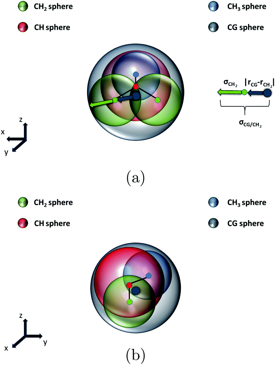
Isotactic polypropylene (iPP) has been simulated both at the united-atom (UA) and the coarse-grained levels (CG). The UA representation, in which carbons and hydrogens are fused into one single atom, as shown in Fig. 1a, is described by the TraPPE-UA force field that was initially developed by Martin and Siepmann³² and then improved by Pütz et al.³³ by introducing an improper dihedral potential that preserves the correct stereochemistry. In the UA model, the non-bonded interactions are calculated for atoms separated by more than three bonds, as TraPPE-UA excludes 1–4 interactions. At the CG level, a single interaction site (bead) comprises a methyl, a methine and two half methylene groups that are shared between adjacent beads (Fig. 1b). The center of the CG site is placed at the center of mass of these groups. The latter representation is invoked in the MARTINI force field²¹ which was refined specifically for polypropylene by Panizon et al.²⁹ In this MARTINI model, the non-bonded interactions between the first and the second neighbors are excluded.

Fig. 1 All-trans configuration of iPP (a) at the united-atom level and (b) at the coarse-grained level. Right-handed helical configuration of iPP (c) at the united-atom level and (d) at the coarse-grained level. The center of mass of the iPP monomer parts which comprise a coarse-grained bead (dashed line) is indicated by a black dot in (a).

Monte Carlo and molecular-dynamics simulations were performed, as explained later, for a single iPP chain (both in a perfect helical structure and coiled), as well as for iPP melts. All the systems, except for the perfect iPP helical structures, were generated using the Amorphous Builder plugin of the Materials and Process Simulation (MAPS) platform developed by Scienomics.³⁴ The perfect iPP helical structures at the UA level were created based on diffraction data from Immirzi and Iannelli,³⁵ in the same way as it has been recently described by Romanos and Theodorou.³⁶

A perfect iPP helical structure, with three iPP monomers per helical turn, can be either left-handed (LH) or right-handed (RH). At the UA level a RH helix can be spotted as sequences of trans (180°) (CH₂–CH–CH₂–CH) and gauche⁻ (−60°) (CH–CH₂–CH–CH₂) dihedral angles along a chain (Fig. 1c) resulting in an up arrangement,³⁷ while a LH helix is spotted as a sequence of gauche⁺ (+60°) (CH₂–CH–CH₂–CH) and trans (180°) (CH–CH₂–CH–CH₂) dihedral angles resulting in a down arrangement.³⁷ For the dihedral angle definition, we make use of the IUPAC convention.³⁸ The two types of helices are enantiomers, meaning that one is the mirror image of the other. It is worth noting that high energy helices do exist and can be defined as a sequence of (trans, gauche⁺) and (gauche⁻, trans).³⁹ In order to represent an iPP helical structure at the CG level, the UA RH and LH helices are mapped based on the mapping proposed by Panizon et al.²⁹ In Fig. 1d, it is clearly seen that the helical structure of the iPP chain persists at the CG level as well. The dihedral angle pattern for a CG helix should also be defined: a RH CG helix is denoted by a sequence of +100° dihedral angles, and a LH CG helix is denoted by a sequence of −100° dihedral angles. At the CG level there is no distinction between high energy helices and low energy helices.

2.2 Simulation methods

The first goal of the present study is to test if the existing MARTINI force field used for modeling iPP at the CG level²⁹ is able to capture the helical behavior of chains. For this purpose, the perfect iPP helical structures are simulated at both the UA and CG levels. The next step is to tailor the current CG force field aiming at the reproduction of melt structural properties both from a single chain MC simulation at the UA level and experimental measurements. The general strategy for developing the new CG force field is shown in Fig. 2. In Fig. 2b, a single UA iPP chain is presented, which will be simulated with MC by mimicking the interactions that a chain feels in an iPP melt (Fig. 2a). Mapping the produced sample of equilibrated UA conformations to the CG level (2c), CG bonded interactions can be extracted. CG non-bonded interactions are adjusted to experimental properties by using a geometric approximation, which is discussed in more detail in Appendix 1. Finally, the validation of the model has been carried out by performing both single chain MC simulations and melt molecular-dynamics simulations at the CG level.

Fig. 2 (a) An iPP melt at the UA level. A single iPP chain is highlighted with blue color. (b) A single UA iPP chain. This representation can serve as input for single unperturbed chain MC simulations. (c) A single CG iPP chain produced by mapping the single UA iPP chain. From this representation the interactions for the new CG force field can be extracted.

2.2.1 Molecular-dynamics simulations. In order to check if helices of different handedness are energetically equally probable, single chain MD simulations have been performed at both UA and CG levels. In detail, single chain simulations of RH and LH helices were carried out at constant low temperature of T = 10 K using the velocity rescaling thermostat.⁴⁰ No boundary conditions were used. Coarse-grained helices were simulated under the same conditions. Then, for testing the ability of the existing MARTINI model²⁹ and the newly developed model to produce iPP melts of RH and LH helices in equal amounts, many-chain iPP melts were simulated in the NPT statistical ensemble at T = 500 K and P = 1 bar using the Nosé–Hoover thermostat and the Parrinello–Rahman barostat.⁴¹ In this case, periodic boundary conditions were used in all directions. The timesteps for the UA and the CG levels were 1 fs and 20 fs,²⁹ respectively. At the CG level, we used the same timestep as suggested in ref. 29, where the MARTINI implementation was discussed. Moreover, for the pair list generation the Verlet algorithm was used⁴² with a cut-off distance of 1.4 nm. For the van der Waals interactions, a straight cut-off was chosen at r_c = 1.2 nm at the UA level with tail corrections and at r_c = 1.1 nm at the CG level with a shift of the potential to zero at the cut-off distance. All the simulations were performed using the Gromacs 5.0.7⁴³ simulation package. More details are given later in the Results section.

2.2.2 Single chain MC simulations. Single chain MC simulations have been carried out for a single iPP chain on both the UA and CG levels at T = 500 K. Four MC moves were implemented according to Tzounis et al.,⁴⁴ each with a specific attempt probability. These MC moves are: (a) translational or single atom displacement (10%),⁴⁵ (b) flip atom move (10%),⁴⁶ (c) pivot move (70%),^47,48 (d) flip branch move (10%). At the CG level, move (d) is omitted, as there is no branch, and the attempt probability of move (c) is increased by 10%.

On both levels (UA and CG), each force field describes explicitly all stretching, bending and torsional interactions. In a full melt simulation, non-bonded interactions would be calculated for atoms both along the same chain (intramolecular) and between different chains (intermolecular). Based on Flory's random coil hypothesis,⁴⁹ however, a chain in a melt behaves as if it is subject to local interactions only. For the purpose of sampling single unperturbed chain conformations representative of the melt, nonlocal intramolecular interactions between topologically distant segments and all intermolecular interactions can be omitted. Thus, to sample a single unperturbed chain, one needs to define precisely what constitutes local interactions. Tzounis et al.⁴⁴ have introduced a way of defining local interactions by systematically varying the range of nonbonded interactions along a chain (Fig. 3). This range is set by a parameter Δn_pair, which determines with how many neighboring monomers a specific monomer interacts and is estimated based on an empirical criterion.⁴⁴ Specifically, the value of Δn_pair which maximizes the chain characteristic ratio is taken as representative of the unperturbed state.⁴⁴ By incorporating these local interactions we are able to sample conformations representative of a melt by simulating just a single chain. Δn_pair was set equal to 3 for both UA and CG simulations based on previous work on polypropylene.⁵⁰

Fig. 3 Definition of local interactions between monomers for single chain MC simulations. Δn_pair corresponds to the number of repeat units to the left and to the right, with which a specific repeat unit interacts. All the atoms belonging to the central repeat unit, marked with a rectangle, interact with all the atoms belonging to the neighboring repeat units, marked with ellipses. Δn_pair = 3 was determined appropriate for polypropylene.⁵⁰

3 Results

3.1 Testing CG MARTINI force field

In this section, the ability of the existing CG MARTINI force field of Panizon et al.²⁹ to produce iPP melts with equally probable RH and LH helices was tested. We started with single iPP helix simulations at the UA and CG level and we proceeded with iPP melt simulations at the CG level. UA RH and LH helices of 18 monomers each were simulated using MD at 10 K for 400 ps in total. The initial helical configurations were mirror images of each other, while a different set of initial velocities was assigned to each helical configuration following a Maxwell distribution. The reason the systems were simulated at such a low temperature is that it was not intended for any of the helices to lose their helical conformation. In particular, we aimed here at the computation of the dihedral energy of the two different helical types.

In Fig. 4a, the evolution of the dihedral energy of the RH and LH UA helices in time is plotted based on the united-atom representation. It is clearly seen that the dihedral energies for each helix fluctuate between the same energy levels. The fluctuations do not alter the helical structure. Next, the two helices were mapped onto a CG representation and a simulation of duration 400 ps was performed. In this case, the dihedral energy for the RH and LH CG helices came out significantly different (Fig. 4b). Even though the helicity is preserved, despite fluctuations, the RH CG helix is energetically higher than the LH helix. Therefore, the MARTINI force field²⁹ favors one helical type (the LH helix) over the other.

Fig. 4 Time evolution of the dihedral energy of single RH and LH helices comprised of 18 monomers each: (a) at the united-atom level using TraPPE-UA³² at 10 K (b) at the coarse-grained level using MARTINI²⁹ at 10 K. In each panel the black line represents the RH helix, while the red line represents the LH helix. The total simulation time was 400 ps for the UA and the CG simulation. The scaling in each graph is different.

To illustrate this further, we performed an MD simulation starting from an iPP CG melt of 40 chains of 50 monomers per chain. The iPP melt was first energy-minimized using the steepest descent algorithm⁵¹ until the maximum force was smaller than 100 kJ mol⁻¹ mm⁻¹. The algorithm converged after approximately 500 steps. Subsequently, a NVT simulation followed for 50 ns and, finally, a NPT simulation was carried out for 1000 ns. The final 500 ns were used for production. The simulation temperature (500 K) is well above the melting temperature for iPP oligomers that has been calculated at 411 K.⁵² The simulated radius of gyration (1.48 nm) and density (1048 kg m⁻³) are in excellent agreement with the results of Panizon et al.²⁹ Note that this density deviates significantly from available experimental data (710–764 kg m⁻³).⁵³

In the CG iPP melt simulated with the MARTINI force field²⁹ we have analyzed the sequences of helical segments along a chain, in order to quantify the length of helical sequences formed spontaneously in the melt. More specifically, a CG segment was characterized as helical if |ϕ + 100°| < 25° (LH) or |ϕ − 100°| < 25° (RH), where ϕ denotes the dihedral angle based on the IUPAC convention.³⁸ A sequence of such dihedrals along the chain is called helical sequence in what follows. In Fig. 5a, the distribution of lengths of helical sequences after 250 ns of NPT MD is plotted for the MARTINI²⁹ model. The percentages in parentheses indicate the fraction of the atoms belonging to either a LH or a RH helix. The initial configuration produced by MAPS had equally distributed helices. As the CG simulation proceeded, the population of the LH helices increased drastically above 40%, while that of RH ones decreased to about 15%. During the whole simulation, the helical sequences remained shorter than 11, the threshold beyond which ordering is initiated.⁵⁴

Fig. 5 MD simulation using MARTINI²⁹ at the CG level for an iPP melt of 40 chains of 50 monomers per chain at 500 K (a) distribution of helical sequence lengths extracted after 250 ns of NPT run. The RH helix is represented in orange and the LH helix in green. The percentages in parentheses indicate the fractions of atoms belonging to either a LH or a RH helix. (b) The probability density function (PDF) P(ϕ) of CG effective dihedral angles. The blue curve presents the results from the present simulations, while the dashed green curve presents the results from Panizon et al.²⁹ The different probabilities are averaged over all configurations.

The overall behavior of the helices is also displayed in the probability density function (PDF) of different CG effective dihedral angles plotted in Fig. 5b. Two maxima can be seen, one at ϕ = −100°, corresponding to the LH helix, and another one at ϕ = +100°, corresponding to the RH helix. The ϕ = −100° peak is clearly higher and thus, by using MARTINI,²⁹ the LH helices in a melt are overpopulated.

3.2 New parametrization of CG dihedral and non-bonded interactions

The main goal now is to validate if the single chain TraPPE-UA-based MC simulation is able to reproduce correctly the structural melt properties and then use it as a reference for an improved CG model which preserves the equal population of both LH and RH helices. Error bars are included only if they are large comparable to the mean values. Otherwise, they are omitted. We simulated a UA single chain of 2000 iPP monomers using MC for 10⁹ steps and the TraPPE-UA force-field, as was described in Section 2.2.2. To begin with, the characteristic ratio C_∞ was calculated as follows:where 〈R²〉 is the mean-square end-to-end distance of the chain, n is the number of chemical backbone bonds and l² is the average squared chemical backbone bond length. C_∞ was estimated at 6.4, while the experimental value reported by Fetters et al.⁵⁵ is 6.2. There is a slight overestimation, but the agreement is acceptable. Available melt iPP simulation results with a different force field reported C_∞ = 5.49 ± 0.33.⁵⁶ The underestimation of C_∞ in ref. 56 can be attributed to the short chain length of the system used there (152 skeletal bonds per chain).

Following Brandrup et al.,⁵⁷ the iPP chain radius of gyration R_g was estimated as

where C = 0.032 mm mol^1/2 g^−1/2 and M is the molecular weight in g mol⁻¹. The resulting value for a 2000 units iPP chain, based on experimental data,⁵⁷ is 9.27 nm. The present simulation gives R_g = 9.8 nm. Overall, the TraPPE-based C_∞ and R_g denote a slightly stiffer chain but overall the results are in a good agreement with experimental and theoretical predictions.

In addition, the helical sequence length distribution for UA iPP is plotted (Fig. 6a), as also done by Yamamoto.³⁹ The iPP configuration was extracted after 5 × 10⁸ MC steps. It is important to note that the populations of both types of helices are equally distributed. Despite having a long chain of 2000 monomers, the helical sequences do not grow to more than 12 monomers per sequence. Thus, this UA model has no preference for any of the helical types, preserves the helical behavior, and reproduces the conformational properties of realistic iPP very well.

Fig. 6 Monte Carlo simulations performed for a single chain of 2000 UA monomers at 500 K using the TraPPE-UA force field: (a) Distribution of helical sequence length. The RH helix is represented with orange and the LH helix with green. The percentages in parentheses represent the fraction of atoms that belong to either a LH or a RH helix. The configuration was extracted after 5 × 10⁸ MC steps. (b) Dihedral effective potential U(ϕ) vs. CG effective dihedral angles. The single unperturbed chain configurations were initially sampled at the UA level using TraPPE-UA and then mapped onto the CG level to obtain the potential of mean force of CG torsion angles. The red curve represents the mapped CG trajectory from TraPPE-UA. A Ryckaert–Bellemans function was fitted to the potential of mean force U(ϕ), and is shown by the black dashed curve. The MARTINI dihedral effective potential U(ϕ) is shown by the blue curve.²⁹

The next step was to use TraPPE-UA results as a reference in order to parametrize the dihedral effective potential for the new CG force field which would preserve the equal distribution of both LH and RH helices. For this purpose, the UA trajectory was mapped onto the CG level. From this mapped CG trajectory the PDF P(ϕ) of dihedral angles was extracted and, subsequently, was converted to the dihedral effective potential, U(ϕ) = −RT ln(cP(ϕ)). The constant c was selected arbitrarily equal to 1000°, as it does not have any effect on the simulation. Then, a Ryckaert–Bellemans function (eqn (5)) was fitted to U(ϕ), as shown in Fig. 6b. In the same figure, the MARTINI dihedral effective potential U(ϕ) is also plotted, where at ϕ = −100°, corresponding to LH helix, the dihedral energy is significantly lower than the dihedral energy at ϕ = 100°, corresponding to RH. The new CG force field comprises effective stretching, bending, torsional and non-bonded interactions, with the parameters presented in Table 1. The reader should note that any coupling between successive effective torsion angles is ignored in the CG model. In other words, the total CG effective torsional potential of a chain is modeled as a sum of terms, each depending on a single effective torsion angle.

Table 1 Parameters for the new coarse-grained HELIPP force field

Stretching interactions (eqn (3))

l _o = 0.298 nm, k_b = 48 000 kJ mol⁻¹ nm⁻²

Bending interactions (eqn (4))

θ ₀ = 119° k_θ = 78 kJ mol⁻¹ rad⁻²

Torsional interactions (eqn (5))

a ₀ = −8.08655 kJ mol⁻¹, a₁ = −2.88516 kJ mol⁻¹, a₂ = 16.61891 kJ mol⁻¹

a ₃ = 0.79249 kJ mol⁻¹, a₄ = −8.79016 kJ mol⁻¹, a₅ = 1.33047 kJ mol⁻¹

Non-bonded interactions (eqn (6))

ε = 2.625 kJ mol⁻¹, σ = 0.53 nm

---

Stretching interactions. The CG stretching interactions are described as:where r_ij denotes the distance between two CG beads connected by a bond with force constant k_b. The mean CG bond length l_o was computed equal to 0.293 nm. The mean bond length used by Panizon et al.²⁹ was 0.298 nm, and we make use of the same k_b and l₀ as they did.²⁹

Bending interactions. The CG bending interactions are described by a Restricted Bending (ReB) potential as proposed by Bulacu et al.,⁵⁸where θ_ijk is the angle that is formed by three CG beads i, j, k, and k_θ is the bending constant. The value of θ_o is 119°, the same as in the iPP MARTINI model.⁵⁸ The reason for selecting the specific potential is the advantage provided by ReB in using longer timesteps and avoiding numerical instabilities that are often encountered in very flexible coarse-grained molecules.⁵⁸

Torsional interactions. The CG effective dihedrals were parameterized based on the single chain Monte Carlo Simulations explained previously in Section 2.2.2. For the fitting, we choose a Ryckaert–Bellemans function,where ϕ_ijkl is the dihedral angle formed by four CG beads i, j, k, l. The parameters extracted from the fitting to the dihedral effective potential curve are noted by a_n.

Non-bonded interactions. For the representation of the non-bonded interactions in the CG model, a Lennard-Jones potential was used,where r_ij is the distance between two interacting particles i and j, σ is the distance at which the energy is zero and ε is the depth of the potential well. We use the same ε as Panizon et al.,²⁹ while we set σ = 0.53 nm, based on a geometric approach (see Appendix 1), in contrast to σ = 0.43 nm used in MARTINI. The non-bonded interactions are calculated both intermolecularly and intramolecularly for CG beads separated by at least four CG beads (monomers).

3.3 Validation of the HELical isotactic polypropylene potential (HELIPP)

To test the HELIPP CG force field, a single unperturbed CG chain of 2000 chemical monomers was simulated by Monte Carlo for 10⁹ steps. The optimal value for Δn_pair was estimated equal to 3. The characteristic ratio C_nvs. the number of real chemical bonds N_b is plotted in Fig. 7. It is obvious that C_n has clearly reached a plateau value for N_b > 3000. The plateau value of C_n calculated by HELIPP equals 5.7, slightly lower than the value measured using TraPPE-UA (6.4). By performing single chain MC simulation using the existing MARTINI force field,²⁹ the estimate was 8.9. So, HELIPP reproduces better the stiffness of the iPP chain than the existing MARTINI CG model²⁹ and yields a characteristic ratio comparable to the experimental results.⁵⁵ All the simulations of the characteristic ratio were carried out at 500 K, while the reference temperature for the experimental measurements was 460 K.⁹ The radius of gyration from single unperturbed chain CG simulations equals 9.23 nm, and is also close to the theoretical calculations.⁵⁷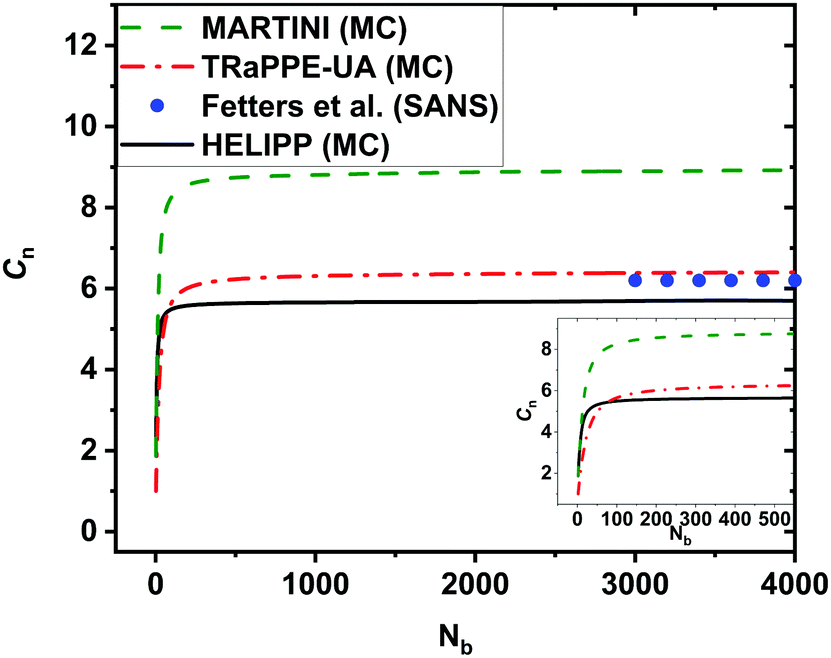

Fig. 7 The characteristic ratio C_nvs. the number N_b of real chemical backbone bonds from Monte Carlo simulations for a single chain of 2000 monomers on both UA and CG levels at 500 K. At the UA level the TraPPE-UA was used, plotted with a red dash-dot line, while at the CG level the new HELIPP potential was used, plotted with black line. Results obtained with the existing MARTINI force field at 500 K²⁹ are also shown as a green dashed line. Experimental values⁵⁵ at 460 K are shown with the blue dots.

Next, the PDF of CG effective valence angles is plotted in Fig. 8a. Looking at the HELIPP curve, a peak is observed at 119°, while the TraPPE-UA curve has a maximum at 109°, which is the most probable one, and a second weaker shoulder at 145°. As the ReB potential used for describing bending interactions⁵⁸ is not able to reproduce a double-peak curve, the two curves do not match each other. The HELIPP curve actually replaces the UA bending angle distribution with a smoothed, unimodal approximate distribution.

Fig. 8 PDF of (a) CG effective valence angles θ and (b) CG effective dihedral angles ϕ for a single chain of 2000 monomers simulated by Monte Carlo using TraPPE-UA (red dash curve), HELIPP (black curve) and MARTINI (blue curve) at 500 K.

In Fig. 8b, the PDF of CG effective dihedral angles is also plotted. In both curves, two maxima can be distinguished. Each peak represents a helical type, both are equally probable. In the regions [−180°, −150°] and [180°, 150°], representing the trans states, the HELIPP curve exhibits a slightly higher probability. On the contrary, in the region [−30°, 30°], which refers to the cis state, the HELIPP curve indicates a lower probability. CG beads, which have a parameter σ from the LJ interactions larger on average than the same parameter of the united atoms they are constituted from (see Appendix 1), experience slightly larger repulsion when approaching each other, which leads to the slightly less probable cis state.

Furthermore, we performed MD simulations of a CG melt of 40 chains of 500 beads each using this new HELIPP force field. In order to equilibrate the system, an energy minimization was undertaken until the maximum force was smaller than 10 kJ mol⁻¹ nm⁻¹, followed by a NVT MD of 5 ns and a NPT MD of duration 5 ms. The simulation temperature T = 500 K was well above the melting temperature of high molar mass iPP (T = 460 K) measured by differential scanning calorimetry.⁹ The simulation pressure P was set to 1 bar using the Parrinello–Rahman barostat.⁴¹ The energy minimization converged after 25 000 steps.

We compare the MD simulation to the Single Chain Monte Carlo simulation with the same HELIPP force field. The PDF for CG effective valence and dihedral angles extracted from the MD simulation match perfectly (not shown here) the ones derived from CG single unperturbed chain MC sampling and shown in Fig. 8. The characteristic ratio from the CG melt MD simulation was estimated equal to 5.87 ± 0.09, close to the value 5.7 from the single CG chain MC simulation. Moreover, the density was measured as 730 kg m⁻³, in a good agreement with experimental results (710–764 kg m⁻³).⁵³

The helical sequence length was also studied. Both types of helices are now equally probable with approximately 30% of the beads belonging to RH helix and 30% to a LH helix during the whole simulation. Neither of them grows longer than 12 monomers per helical sequence. So, HELIPP is able to reproduce LH and RH helices in equal amounts and that holds even for rather long simulations on the μs scale.

Subsequently, using this new coarse-grained model, the entanglement molecular weight M_e was calculated by performing a topological analysis on the trajectory produced during the last 1 μs of the simulation. For the topological analysis, the CReTA (Contour Reduction Topological Analysis) algorithm⁵⁹ was used. This algorithm maps an entangled polymer system to its corresponding system of primitive paths, having the same topological constraints as the original system. M_e was computed equal to 4432 ± 121 g mol⁻¹, whereas in experiments carried out for iPP melt M_e was estimated between 5100–5500 g mol^−1 60 and 6900 g mol⁻¹.⁶¹ So HELIPP produces slightly more entangled system in comparison to the experiments, but no comparison was made with other simulations, as no data were available.

Finally, we have calculated the cohesive energy of the iPP melt which can be expressed by the Hildebrand solubility parameter δ.⁶²δ can be obtained as

where E_coh is the cohesive energy, n is the number of molecules, V_cell the volume of the simulation box, N_A Avogadro's number, U_i,LJ the intramolecular LJ interactions energy of a single chain and U_cell,LJ the intramolecular and intermolecular LJ interactions energy in the simulation box. The angular brackets denote ensemble averaging.

In order to calculate δ for different temperatures, we performed multiple NPT MD simulations for 10 ns for a system of 40 chains of 50 monomers per chain using the HELIPP and TraPPE-UA force fields. The simulation temperatures were T = 400, 450 and 500 K, close to the temperature at which the HELIPP force field has been developed. The temperature dependence of the solubility parameter is plotted in Fig. 9. It can be seen that at T = 475 K, δ = 14.2 MPa^1/2 obtained from HELIPP and δ = 10 MPa^1/2 from TraPPE-UA force field. Comparing with other experimental (δ = 15.2 MPa^1/2)⁶³ and simulation data (δ = 14.8 MPa^1/2)⁵⁶ at T = 475 K, HELIPP seems to reproduce the solubility parameter much better than TraPPE-UA. At T = 298 K, the experimental value⁶⁴ varies from 16.8 to 18.8 MPa^1/2, while the present estimation with HELIPP is 15.5 MPa^1/2, showing a larger deviation at this temperature. So HELIPP reproduces well the solubility parameter above the melting temperature, even better than simulations at the UA level.

Fig. 9 The solubility parameter plotted at different temperatures for an iPP of 40 chains of 50 monomers per chain. The solubility was calculated both at the UA level with TraPPE-UA (black squares) and at the CG level with HELIPP (green dots) using molecular-dynamics simulations. The experimental values obtained from Maier et al.⁶³ and from van Krevelen⁶⁴ are plotted with a magenta inverse triangle and a red rhombus, respectively, while atomistic simulation results obtained by Logotheti et al.⁵⁶ are plotted with a blue triangle.

4 Discussion

In this study we have developed a new CG force field for iPP melts, named HELIPP, which reproduces structural properties sufficiently well and, most importantly, is able to capture the different handedness of the iPP helices. HELIPP is remarkably simple and quite friendly to be adopted in simulations, as only one type of torsional angle is used and non-bonded interactions are described by a single LJ σ and a single LJ ε value. This force field could be possibly extended to other ordered polymer structures, as the approach we have developed is applicable not only for iPP melts. Furthermore, we have presented a method for developing such a CG model based on a single unperturbed chain MC algorithm and we discuss the possibility of using this method for polymers of rather arbitrary structure.

The representation of the RH and LH helices at the CG level and preservation of the handedness have been proved essential for the modeling of iPP melts. The existing MARTINI CG force field for iPP²⁹ is not able to reproduce correctly the two different helical types and overestimates the stiffness of the chains and the density. By introducing the CG iPP helices and tailoring the dihedral effective potential so that none of the helices is favored over the other, we managed to have a more accurate estimation for the iPP chain characteristic ratio, C_∞ = 5.7. Moreover, by re-adjusting the Lennard-Jones σ based on a geometric approximation, as discussed in Appendix 1, the density ρ = 730 kg m⁻³ was also improved. This force field was applied to an iPP melt but seems promising also for iPP semi-crystalline morphology. Below we present a snapshot of a lamella formation after an iPP coarse-grained system was submitted to stretch-induced crystallization using the HELIPP. Specifically, a system consisting of 20 chains of 1000 CG monomers each was equilibrated in the NPT statistical ensemble at T = 500 K and P = 1 bar using the Nosé–Hoover thermostat and the Parrinello–Rahman barostat.⁴¹ Then, it was cooled down to T = 380 K with cooling rate 10 K ns⁻¹ and stretched at the same temperature to 5 times its initial length in the Nė_xxP_yyP_zzT statistical ensemble with stretching rate ė_xx = 10⁷ s⁻¹. Finally, it was annealed in the NL_xxP_yyP_zzT statistical ensemble at T = 380 K for 400 ns (Fig. 10).

Fig. 10 A lamella snapshot of a CG system of 20 chains of 1000 CG monomers each using the HELIPP after a stretch-induced crystallization simulation.

iPP crystals consist of lamellae which are formed by RH and LH helices in equal amounts. This characteristic is possible to maintain now at the CG level, although attention should be paid to two main aspects: (1) the presented force field has not been tested thoroughly for temperatures below the melting point. (2) At these low temperatures the reproduction of the different iPP crystal phases is crucial, and also has not been tested yet.

Single unperturbed chain MC simulations have been used for the fast and effective estimation of the stiffness of polymer melts but, as far as we know, not for the development of a force field up until now. The CG stretching, bending and torsional interactions can be accurately derived from a single chain MC simulation. In the present study we tailored only dihedral and non-bonded interactions, based on the approach implemented by Panizon et al.²⁹ For bending interactions we adopted the Restricted Bending (ReB) potential. In addition to the work presented above, we have performed CG simulations with tabulated potentials both for bending and torsional interactions which perfectly match the PDF of the CG effective valence and dihedral angles derived from TraPPE-UA single chain MC simulation (Fig. 8a). The results using tabulated potentials can be found in the ESI.† The main reasons we did not use these potentials for the production simulations were: (1) tabulated potentials can not be easily implemented in different simulation packages. (2) The maximum timestep we had to use with the tabulated potentials was 5 fs, while with ReB we use a timestep of 20 fs. For these reasons, we incorporated ReB and Ryckaert–Bellemans potential into HELIPP. As far as the non-bonded interactions are concerned, here we used a geometric approach which proved to be effective (see Appendix 1). This geometric approach is recommended to be tested also for other polymer systems. Another method that could be used for mapping non-bonded interactions is iterative Boltzmann inversion,⁶⁵ but, overall, the single chain Monte Carlo method can serve as a new coarse-graining method for mapping a variety of polymer melt models to the coarse-grained level.

Finally, we demonstrate the computational significance of the coarse-graining by comparing a UA and a CG simulations in terms of time. Coarse-grained models are far more efficient computationally than models with higher resolution. To check this, we simulated 20 iPP chains of 500 monomers per chain at the UA level using TraPPE-UA and at the CG level using the HELIPP. The simulations were carried out on a cluster made of 504 nodes comprised of 128 AMD Rome 7H12 processors, each with 2.6 GHz and 2 GB per core. The estimation made on 32 cores on 1 node for the CG performance was 4000 ns day⁻¹, while for the UA the performance was 100 ns day⁻¹. So, the CG iPP model performs 40 times faster than the UA iPP model.

5 Conclusions

The main scope of this research was to integrate the helical behavior of iPP into a coarse-grained model. For this reason, we developed a model that accounts indirectly for the influence of the iPP branch which is translated to different helical conformations along the chains. We showed that, even in melts, where the helical segments are short, the incorporation of helicity improves significantly the structural properties of iPP. In order to develop a new CG force field (HELIPP) that preserves helices, we implemented a coarse-grained method based on a single chain Monte Carlo algorithm which proved to be effective. Using the new HELIPP force field, long iPP chains were sufficiently relaxed in the melt by ms-long simulations and the characteristic ratio was accurately measured. In this way, slow relaxation above the melting temperature has been circumvented. In the future it would be interesting to extract dynamical properties as well from the new CG model. Furthermore, given that HELIPP captures the helical behavior of iPP which is essential for structural ordering and performs really well in terms of CPU time, studies of crystallization by molecular simulations using the new HELIPP model is an immediate objective for future work.

Conflicts of interest

There are no conflicts of interest to declare.

Appendix 1

Calculation of the coarse-grained Lennard-Jones σ_CG parameter

In order to calculate the radius σ_CG at which the non-bonded LJ potential energy for coarse-grained particles is zero, we followed a geometric approximation. Given a bunch of united-atom LJ spheres with specific radius σ, the problem is to find the radius σ_CG of a coarse-grained LJ sphere with its center lying at the center of mass of these united atoms, that is approximately tangential to the sphere of each individual united-atom. In the present case, the united atoms that form a coarse-grained bead are: a methyl group (CH₃), a methine group (CH) and two half-methylene groups (CH₂). These united atoms can be placed in a Cartesian coordinate system with the methine group lying at the origin. The positions of the remaining united atoms are calculated according to the bond length and valence angles given by Pütz et al.,³³

r_CH = {0,0,0}

r_CH2 = { −0.129, 0, −0.084}

r_CH3 = {0, 0.122, 0.094}

The position of the coarse-grained bead is calculated by the center of the mass of the united atoms,

r_CG = {0, 0.044, 0.001}

All coordinates have been calculated in nm.

In Fig. 11, the radius of the coarse-grained LJ sphere σ_CG/CH2 that is tangential to the LJ sphere of the methylene group and has its center at the position of the coarse-grained bead is calculated,

Fig. 11 Lennard-Jones spheres of the united atoms and the coarse-grained bead. The coarse-grained LJ sphere with radius σ_CG is sketched in grey color, the methyl united-atom LJ sphere with radius σ_CH3 in blue color, the methylene united-atom LJ sphere with radius σ_CH2 in green color and the methine united-atom LJ sphere with radius σ_CH in red color. Each colored dot represents the center position of either the united atoms or the coarse-grained bead. (a) Profile view (b) side view.

σ _CG/CH2 = ‖r_CG − r_CH2‖ + σ_CH2 = 0.56 nm

, where r_CG is the position of the coarse-grained bead (black dot in Fig. 11), r_CH2 is the position of the methylene group (green dot in Fig. 11) and σ_CH2 is the distance at which the Lennard-Jones potential energy for the methylene united-atom is zero (green arrow in Fig. 11).

Similarly, σ_CG/CH3 = 0.49 nm and σ_CG/CH = 0.51 nm. All the distances at which the LJ potential becomes zero for the united atoms are given by Pütz.³³

Finally, σ_CG is calculated as the average of:

Acknowledgements

This research forms part of the research programme of DPI, project #831. This work was carried out on the Dutch national e-infrastructure with the support of SURF Cooperative. We also thank DPI industrial partners for helpful discussions.

References

1. American Chemical Society National Historic Chemical Land-marks, Polypropylene and High-density Polyethylene, http://www.acs.org/content/acs/en/education/whatischemistry/land-marks/polypropylene.html, Accessed: 2021-10-15.
2. P. Wambua, J. Ivens and I. Verpoest, Compos. Sci. Technol., 2003, 63, 1259–1264.
3. S. Y. Fu, B. Lauke, E. Mäder, C. Y. Yue and X. Hu, Composites, Part A, 2000, 31, 1117–1125.
4. M. Ramos, A. Jiménez, M. Peltzer and M. C. Garrigós, J. Food Eng., 2012, 109, 513–519.
5. F. Di Sacco, M. Gahleitner, J. Wang and G. Portale, Polymers, 2020, 12, 1636.
6. W. Hufenbach, R. Böhm, M. Thieme, A. Winkler, E. Mäder, J. Rausch and M. Schade, Mater. Des., 2011, 32, 1468–1476.
7. H. A. Maddah, Am. J. Polym. Sci., 2016, 6, 1–11.
8. Z. Wang, Z. Ma and L. Li, Macromolecules, 2016, 49, 1505–1517.
9. K. Yamada, M. Hikosaka, A. Toda, S. Yamazaki and K. Tagashira, Macromolecules, 2003, 36, 4790–4801.
10. K. N. Okada, J. I. Washiyama, K. Watanabe, S. Sasaki, H. Masunga and M. Hikosaka, Polymer, 2010, 42, 464–473.
11. M. Destrée, F. Lauprêtre, A. Lyulin and J. P. Ryckaert, J. Chem. Phys., 2000, 112, 9632–9644.
12. T. Miyoshi, A. Mamun and W. Hu, J. Phys. Chem. B, 2009, 114, 92–100.
13. S. J. Antoniadis, C. Samara and D. N. Theodorou, Macromolecules, 1998, 31, 7944–7952.
14. V. K. Kuppa, P. J. Veld and G. C. Rutledge, Macromolecules, 2007, 40, 5187–5195.
15. E. D. Akten and W. L. Mattice, Macromolecules, 2001, 34, 3389–3395.
16. C. Luo, Polym. Cryst., 2020, 3, e10109.
17. H. Wang, C. Junghans and K. Kremer, Eur. Phys. J. E: Soft Matter Biol. Phys., 2009, 28, 221–229.
18. D. Kauzlariç, J. T. Meier, P. Español, S. Succi, A. Greiner and J. G. Korvink, J. Chem. Phys., 2011, 134, 64106.
19. N. J. H. Dunn and W. G. Noid, J. Chem. Phys., 2015, 143, 243148.
20. T. Mulder, V. Harmandaris, A. V. Lyulin, N. F. Van Der Vegt and M. A. Michels, Macromol. Theory Simul., 2008, 17, 393–402.
21. S. J. Marrink, H. J. Risselada, S. Yefimov, D. P. Tieleman and A. H. De Vries, J. Phys. Chem. B, 2007, 111, 7812–7824.
22. F. A. Detcheverry, D. Q. Pike, U. Nagpal, P. F. Nealey and J. J. de Pablo, Soft Matter, 2009, 5, 4858–4865.
23. B. A. P. Betancourt, J. Douglas and F. W. Starr, Soft Matter, 2012, 9, 241–254.
24. Y. An, K. K. Bejagam and S. A. Deshmukh, J. Phys. Chem. B, 2018, 122, 7143–7153.
25. L. Gao and W. Fang, J. Chem. Phys., 2011, 135, 184101.
26. K. S. Schweizer, E. F. David, C. Singh, J. G. Curro and J. J. Rajasekaran, Macromolecules, 1995, 28, 1528–1540.
27. K. S. Schweizer and J. G. Curro, Phys. Rev. Lett., 1987, 58, 246–249.
28. T. Haliloğlu and W. L. Mattice, J. Chem. Phys., 1998, 108, 6989–6995.
29. E. Panizon, D. Bochicchio, L. Monticelli and G. Rossi, J. Phys. Chem. B, 2015, 119, 8209–8216.
30. C. Wu, R. Wu, W. Xia and L. Tam, J. Polym. Sci., Part B: Polym. Phys., 2019, 57, 1779–1791.
31. C. Wu, R. Wu and L. Tam, Nanotechnology, 2021, 32, 32.
32. M. G. Martin and J. I. Siepmann, J. Phys. Chem., 1999, 103, 4508–4517.
33. M. Pütz, J. G. Curro and G. S. Grest, J. Chem. Phys., 2001, 114, 2847–2860.
34. D. N. Theodorou and U. W. Suter, Macromolecules, 2002, 18, 1467–1478.
35. A. Immirzi and P. Iannelli, Macromolecules, 1988, 21, 768–773.
36. N. A. Romanos and D. N. Theodorou, Macromolecules, 2010, 43, 5455–5469.
37. M. Hikosaka and T. Seto, Polym. J., 1973, 5, 111–127.
38. G. P. Moss, Pure Appl. Chem., 1996, 68, 2193–2222.
39. T. Yamamoto, Macromolecules, 2014, 47, 3192–3202.
40. L. V. Woodcock, Chem. Phys. Lett., 1971, 10, 257–261.
41. M. Parrinello and A. Rahman, J. Appl. Phys., 1981, 52, 7182–7190.
42. L. Verlet, Phys. Rev., 1967, 159, 98–103.
43. D. V. D. Spoel, E. Lindahl, B. Hess, G. Groenhof, A. E. Mark and H. J. C. Berendsen, J. Comput. Chem., 2005, 26, 1701–1718.
44. P. N. Tzounis, S. D. Anogiannakis and D. N. Theodorou, Macromolecules, 2017, 50, 4575–4587.
45. D. Frenkel and B. Smit, Understanding Molecular Simulation, Academic Press, Inc., USA, 2nd edn, 2001.
46. V. G. Mavrantzas and D. N. Theodorou, Macromolecules, 1998, 31, 6310–6332.
47. M. Lal, Mol. Phys., 1969, 17, 57–64.
48. N. Madras and A. D. Sokal, J. Stat. Phys., 1988, 50, 109–186.
49. P. J. Flory, Principles of Polymer Chemistry, Cornell University Press, Ithaka, N.Y., 1953.
50. P. N. Tzounis, D. V. Argyropoulou, S. D. Anogiannakis and D. N. Theodorou, Macromolecules, 2018, 51, 6878–6891.
51. J. C. Meza, Wiley Interdiscip. Rev.: Comput. Stat., 2010, 2, 719–722.
52. P. Pino, P. Cioni and J. Wei, J. Am. Chem. Soc., 1987, 109, 6189–6191.
53. H. M. Freischmidt, R. A. Shanks, G. Moad and A. Uhlherr, J. Polym. Sci., Part B: Polym. Phys., 2001, 39, 1803–1814.
54. X. Chen, S. Kumar and R. Ozisik, J. Polym. Sci., Part B: Polym. Phys., 2006, 44, 3453–3460.
55. J. L. Fetters, D. J. Lohse, A. G. F. César, P. Brant and D. Richter, Macromolecules, 2002, 35, 10096–10101.
56. E. G. Logotheti and D. N. Theodorou, Macromolecules, 2007, 40, 2235–2245.
57. J. Brandrup, E. H. Immergut, E. A. Grulke, A. Abe and D. R. Bloch, Polymer Handbook, Wiley, 1989, vol. 7.
58. M. Bulacu, N. Goga, W. Zhao, G. Rossi, L. Monticelli, X. Periole, D. P. Tieleman and S. J. Marrink, J. Chem. Theory Comput., 2013, 9, 3282–3292.
59. C. Tzoumanekas and D. N. Theodorou, Macromolecules, 2006, 39, 4592–4604.
60. A. Eckstein, J. Suhm, C. Friedrich, R. D. Maier, J. Sassmannshausen, M. Bochmann and R. Mülhaupt, Macromolecules, 1998, 31, 1335–1340.
61. L. J. Fetters, D. J. Lohse and W. W. Graessley, J. Polym. Sci., Part B: Polym. Phys., 1999, 37, 1023–1033.
62. M. Belmares, M. Blanco, W. A. Goddard, R. B. Ross, G. Caldwell, S. Chou, J. Pham, P. M. Olofson and C. Thomas, J. Comput. Chem., 2004, 25, 1814–1826.
63. R. D. Maier, R. Thomann, J. Kressler, R. Mulhaupt and B. Rudolf, J. Polym. Sci., Part B: Polym. Phys., 1997, 35, 1135–1144.
64. D. W. Van Krevelen and K. Te Nijenhuis, Properties of Polymers, Elsevier Science, 2009.
65. D. Reith, M. Pütz and F. Müller-Plathe, J. Comput. Chem., 2003, 24, 1624–1636.

---

Footnote

† Electronic supplementary information (ESI) available: Molecular-dynamics simulations performed using tabulated coarse-grained valence and dihedral angle potentials for isotactic polypropylene melt. See DOI: 10.1039/d2sm00200k

---