
 Open Access Article
 This Open Access Article is licensed under a
 Creative Commons Attribution 3.0 Unported Licence
On the cross-streamline lift of microswimmers in viscoelastic flows†
Akash
Choudhary
 * and
Holger
Stark
*
* and
Holger
Stark
*
Institute of Theoretical Physics, Technische Universität Berlin, 10623 Berlin, Germany. E-mail: a.choudhary@campus.tu-berlin.de; holger.stark@tu-berlin.de
First published on 24th November 2021
Abstract
The current work studies the dynamics of a microswimmer in pressure-driven flow of a weakly viscoelastic fluid. Employing a second-order fluid model, we show that a self-propelling swimmer experiences a viscoelastic swimming lift in addition to the well-known passive lift that arises from its resistance to shear flow. Using the reciprocal theorem, we evaluate analytical expressions for the swimming lift experienced by neutral and pusher/puller-type swimmers and show that they depend on the hydrodynamic signature associated with the swimming mechanism. We find that, in comparison to passive particles, the focusing of neutral swimmers towards the centerline can be significantly accelerated, while for force-dipole swimmers no net modification in cross-streamline migration occurs.
Biological microswimmers are ubiquitous in polymeric media such as cervical, bronchial, and intestinal mucus films.1,2 During the generation of biofilms most bacteria release a mixture of proteins, DNA, and polysaccharides, endowing the fluid with viscoelastic properties,3,4 which significantly alter the swimmer's dynamics.5,6 Pathogens like ulcer-causing Helicobacter pylori survive in a harsh acidic environment by altering the rheology of the mucus lining in the stomach.7 Several theoretical and experimental studies on the dynamics of motile microorganisms in Newtonian flows have revealed their rich dynamics and ability to swim against fluid flows, which aids in seeking nutrients and in reproduction.8–15
Although recent works have provided insights into self-propulsion in non-Newtonian environments,15–32 few have studied the impact of fluid rheology on the dynamics of microswimmers in confined flows.33–36 Mathijssen et al.33 developed a model to predict the dynamical states of microswimmers in non-Newtonian Poiseuille flows. Employing a second-order fluid model, they demonstrated that normal-stress differences reorient the swimmers to cause centerline upstream migration (rheotaxis). This suggests that non-Newtonian properties can help microorganisms evade the boundary accumulation, prevalent in quiescent Newtonian fluids.37,38
The evidence of centerline reorientation of microswimmers can be traced back to pioneering studies on viscoelastic focusing of passive particles in Poiseuille flows.39–41 These studies showed that normal stresses exert a lift force that focuses the particles on the centerline. Ho and Leal41 used the reciprocal theorem and derived an analytical expression for this lift in weakly elastic Boger fluids. The study suggested that the hydrodynamic disturbances around the particle produce a hoop stress that, in the presence of non-uniform shear rate, generates a cross-streamline lift. Recent progress in electrophoresis42–44 has also shed light on the importance of hydrodynamic disturbances in determining these lift forces.
Active microswimmers, as opposed to passive particles, generate additional disturbance flow fields in the fluid due to their self-propulsion. Therefore, the associated lift force or velocity should also have an active component that is characteristic of the self-propulsion mechanism. Since this component is absent in the recently proposed models,33 in this communication we derive the ‘swimming lift’ in a second-order fluid (SOF), and show how it affects the dynamics of a microswimmer in the Poiseuille flow of a viscoelastic fluid. We choose the SOF model because it provides an asymptotic approximation for a majority of slow and slowly varying viscoelastic flows.45,46
Fig. 1 shows a spherical swimmer of radius a at position r that self-propels with velocity vs = vsp in a two-dimensional pressure-driven flow vf = vm[1 − (x/w)2]ez, where vm is the maximum flow velocity and w is the half channel width. The flow profile of the second-order fluid is identical to Poiseuille flow but the pressure field varies in the x-direction.41 In the absence of noise, the swimmer's dynamics is governed by
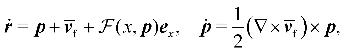 | (1) |
![[v with combining macron]](https://www.rsc.org/images/entities/b_i_char_0076_0304.gif) f = vf/vs,
f = vf/vs, ![[v with combining macron]](https://www.rsc.org/images/entities/i_char_0076_0304.gif) m = vm/vs), lengths by w, and time by w/vs.
m = vm/vs), lengths by w, and time by w/vs.  denotes the total viscoelastic lift velocity, which comprises the passive and swimming lift. Below, we derive the analytical expressions for the lift velocities. We note that normal stresses also modify the particle rotation and the drift velocity along the channel axis. We evaluated these modifications and found that they do not play a significant role in determining the swimmer dynamics.
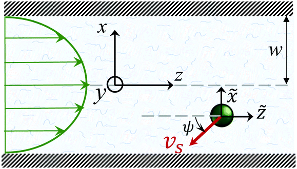 | ||
Fig. 1 A spherical microswimmer with velocity vsp moves in a pressure-driven flow of a second-order fluid inside a channel with half width w. The coordinate frame {![[x with combining tilde]](https://www.rsc.org/images/entities/i_char_0078_0303.gif) ,ỹ, ,ỹ,![[z with combining tilde]](https://www.rsc.org/images/entities/i_char_007a_0303.gif) } co-moves with the swimmer. } co-moves with the swimmer. | ||
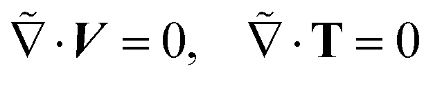
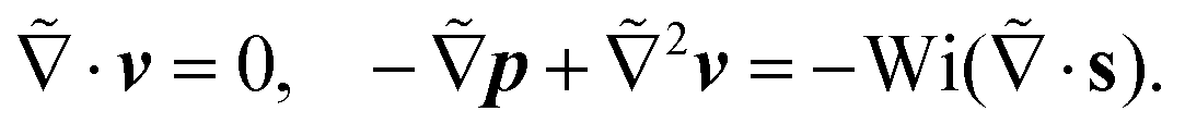
The inertia-less or creeping flow hydrodynamics is governed by the continuity equations for mass and momentum, which we formulate here in the co-moving swimmer frame {,ỹ,} as:
 | (2) |
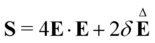 is non-linear in E and contains the lower-convected time derivative of E denoted by Δ. The viscometric parameter δ = −Ψ1/2(Ψ1 + Ψ2) generally varies from −0.5 to −0.7 for most viscoelastic fluids.47–49
We now focus on determining the lift velocity of a microswimmer that disturbs the background flow in two ways. First of all, the microswimmer resists straining by the flow and second, it generates a flow field characteristic of its swimming mechanism, for which we first take a source-dipole swimmer. We split the total velocity field (V = v∞ + v) into background flow field v∞ (in our case the Poiseuille flow in the co-moving swimmer frame) and disturbance field v, and adopt the same nomenclature for the polymeric stress tensor, S = s∞ + s, where s is the polymeric stress tensor associated with the disturbance flow field. We show its full form in the ESI.† Substituting this in the governing eqn (2) yields the equation for the disturbance field v:
 | (3) |
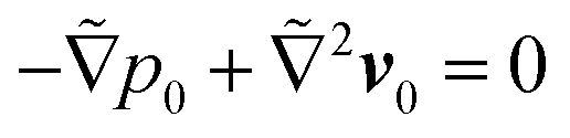 and
and 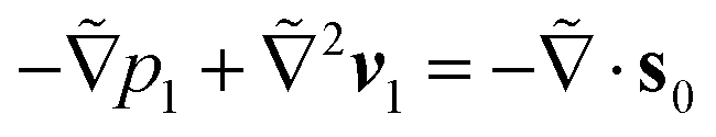 for the first order. Following earlier works on viscoelastic lift,41,43 we use the reciprocal theorem to attain the lift velocity from the first-order problem,
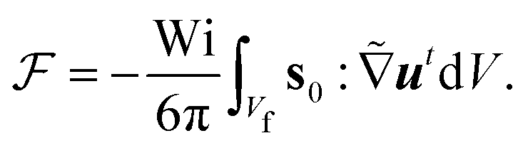 | (4) |
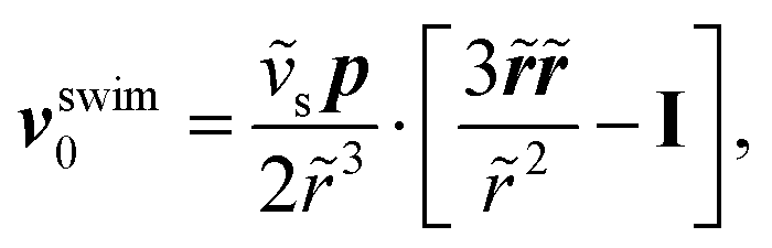 and (ii) the passive disturbance field vpassive0, where ṽs = vs/(vmκ). For the latter, the leading contribution is the stresslet, while higher-order terms due to the curvature in the Poiseuille flow profile are obtained from Lamb's general solution.53 The bounding channel walls modify these bulk flow fields. However, by using the method of reflections for small particles (κ ≪ 1), one can show that they do not alter the lift velocity in leading order in κ.43 Therefore, it is sufficient to perform the integration in eqn (4) in the infinite domain. Using the s0 corresponding to Stokes velocity field in eqn (4), results in the viscoelastic lift velocity given in units of vs:
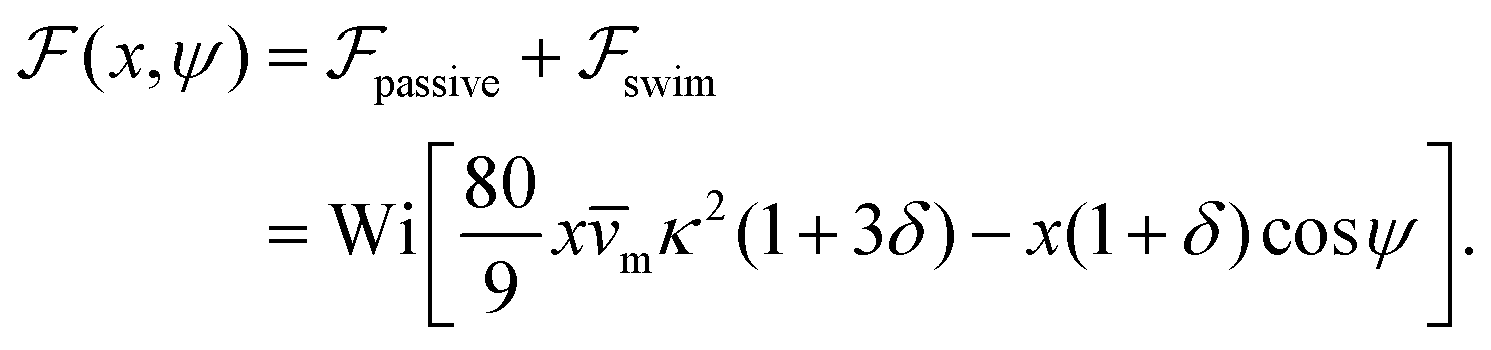 | (5) |
 .41 By fixing δ to a widely-used value of −0.5 (i.e. Ψ2 = 0), we observe that
  focuses the swimmer towards the centerline. The second component is the swimming lift
  that arises due to the source-dipole disturbance created by the neutral swimmer. We note two striking features of
  : the dependence on swimmer orientation through cos
![[thin space (1/6-em)]](https://www.rsc.org/images/entities/char_2009.gif) ψ and that its magnitude is larger by a factor κ−2 compared to the first term.‡
ψ and that its magnitude is larger by a factor κ−2 compared to the first term.‡
Now, we substitute  into the dynamic eqn (1) and examine the effect of
  on the microswimmer dynamics. We find two fixed points in the x–ψ plane at x = 0, with the microswimmer oriented upstream (ψ = 0) or downstream (ψ = ±π). A linear stability analysis provides the following eigenvalues for these fixed points:
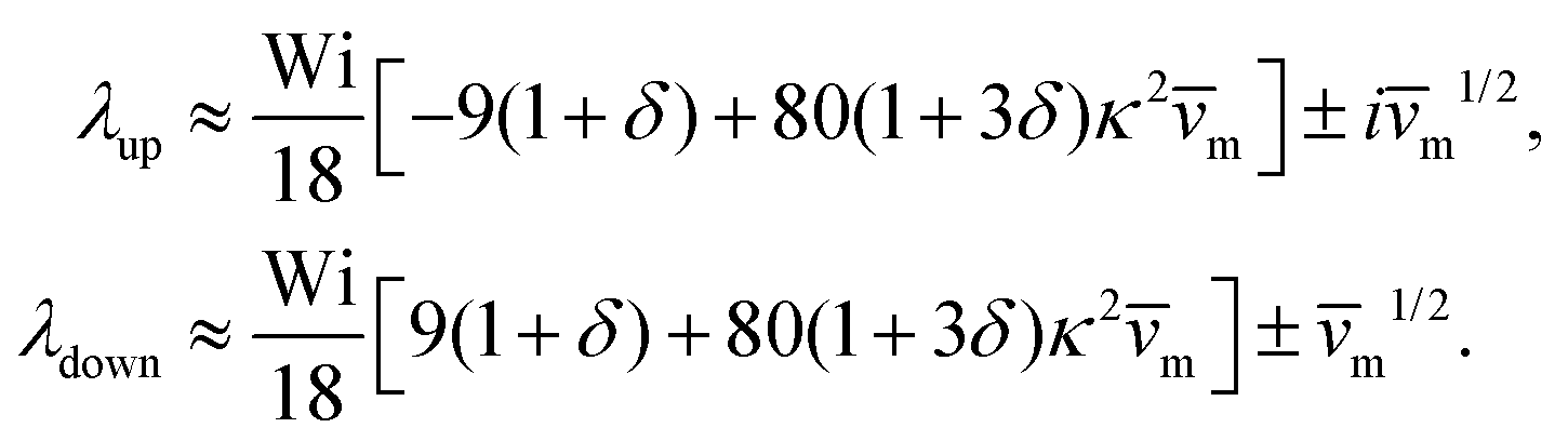 | (6) |
 and
and  . The strong swimming lift helps the neutral microswimmer reach the centerline more rapidly, as suggested by the factor of κ−2 in eqn (5). To quantify this accelerated focusing, we calculate the focusing time τ as the time required for the oscillatory amplitudes to decrease to 5% of the half channel width, i.e., x = 0.05. For upstream swimming at low flow rate (m = 0.9), Fig. 2(c) shows how the focusing time changes with initial position and orientation. We further evaluate the impact of
  on the focusing time in Fig. 2(d). At low flow rates (m ∼ 1), the centerline focusing is much faster when
  is taken into account, however, this difference withers as the flow rate increases; this can also be observed from the analytical expression (5). We further analyze the focusing time over a wider range of parameters in the ESI.†
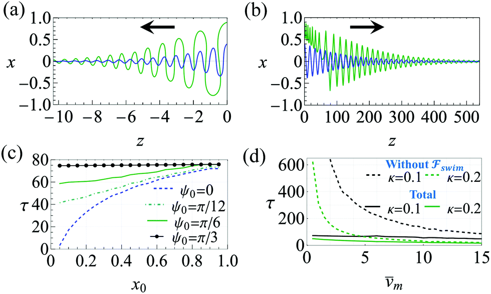 | ||
Fig. 2 Trajectories showing the centerline focusing of a neutral (source-dipole) swimmer oriented upstream while (a) swimming upstream (m = 0.9, ←) and (b) swimming downstream (m = 8, →). The blue and green trajectories only differ in the initial condition x0; for both trajectories we choose ψ0 = 0. Other parameters: Wi = 0.1, κ = 0.1, δ = −0.5. (c) Variation of focusing time τ for different initial conditions x0 and ψ0. Parameters: m = 0.9, Wi = 0.1, κ = 0.1. Trajectories are considered focused when the amplitude of oscillations reaches x = 0.05. (d) Focusing time for various flow rates and two different  swimmer sizes. Dashed lines depict the focusing time in the absence of swimmer sizes. Dashed lines depict the focusing time in the absence of  . We plot the maximum focusing time that occurs for the initial condition x0 = 0.9, ψ0 = 0. . We plot the maximum focusing time that occurs for the initial condition x0 = 0.9, ψ0 = 0. | ||
Now, we shift our attention from neutral squirmers to flagellated microorganisms, such as E. coli and Chlamydomonas, that generate a force-dipole field at the leading order:37,54 . Here
  is the force-dipole strength in units of 8πμa2vs, which depends on the swimming mechanism.37,55,56 Earlier studies on E. coli56,57 and Chlamydomonas58 suggest that
  varies roughly between 0.04 and 0.3. Following the procedure outlined for a source-dipole swimmer, we obtain the swimming lift velocity of the force-dipole swimmer in the units of vs as
 | (7) |
 , it does not result in net cross-stream migration because it is independent of lateral position. The trajectories in Fig. 3(a) and (b) show the dynamics of a force-dipole swimmer. In the steady state, the swimmer shows a stable upstream orientation and swims along the centerline since a deviation from ψ = 0 is counteracted by flow vorticity. For ψ = 0,
  vanishes and the focusing along the centerline is purely due to
  .
.
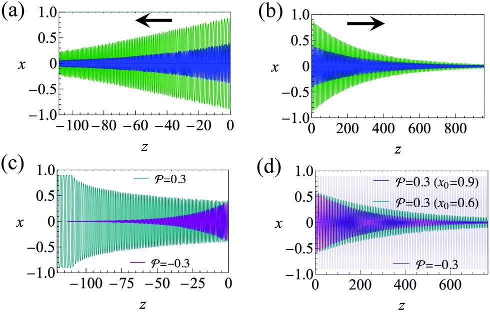 | ||
Fig. 3 Trajectories showing the centerline focusing of pusher  in (a) upstream swimming (m = 0.9, ←) and (b) downstream swimming (m = 3, →). The trajectories for a puller are similar. The blue and green trajectories in (a) and (b) only differ in the initial condition x0; for both trajectories we choose ψ0 = 0. (c) Upstream (m = 0.9) and (d) downstream trajectories (m = 3) with hydrodynamic wall interactions (8) incorporated. For the initial condition, x0 = 0.9, the blue trajectory in the background of (d) shows downstream swinging across the whole channel cross section. We employ hard-core repulsion at the walls. Other parameters: Wi = 0.1, κ = 0.1, δ = −0.5. in (a) upstream swimming (m = 0.9, ←) and (b) downstream swimming (m = 3, →). The trajectories for a puller are similar. The blue and green trajectories in (a) and (b) only differ in the initial condition x0; for both trajectories we choose ψ0 = 0. (c) Upstream (m = 0.9) and (d) downstream trajectories (m = 3) with hydrodynamic wall interactions (8) incorporated. For the initial condition, x0 = 0.9, the blue trajectory in the background of (d) shows downstream swinging across the whole channel cross section. We employ hard-core repulsion at the walls. Other parameters: Wi = 0.1, κ = 0.1, δ = −0.5. | ||
So far we have neglected the hydrodynamic interactions of microswimmers with the bounding channel walls. For force-dipole swimmers, the hydrodynamic wall interactions add a modification of order κ2 and κ3 to the evolution equations of position and orientation, respectively:11,59
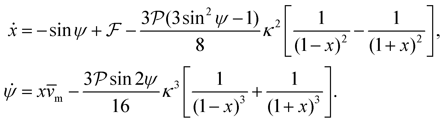 | (8) |
 and results in swinging across the whole channel cross section, where the strong vorticity near the walls always re-orients the swimmer away from it. In contrast, for downstream swimming at larger flow rates [Fig. 3(d)],
  competes with the hydrodynamic wall interactions, which results in some trajectories focusing at the centerline and some following channel-wide swinging depending on the initial condition. The state diagram in Fig. 4(a) illustrates this behavior of pushers for a wide range of parameters. At low flow rates (region I) hydrodynamic wall interactions dominate and thus channel-wide swinging occurs. As the flow rate increases the system enters region II. Here, the realized trajectories depend on the initial condition as depicted in Fig. 3(d): swimmers starting near the walls follow downstream swinging across the channel cross-section, whereas swimmers near the center focus at the centerline. A further increase in flow rate or swimmer size increases the magnitude of
  relative to wall effects, which results in centerline focusing (region III). For the same reason, as the force-dipole strength decreases [see Fig. 4(b)], the regions of swinging state (region I) and coexisting states (region II) shrink. Pullers, on the other hand, are hydrodynamically repelled from the walls11 and therefore always complement
  in centerline focusing [Fig. 3(c) and (d)]. We note that for source-dipole swimmers the hydrodynamic wall interactions are weaker compared to force dipoles since they scale with κ3, and therefore hardly influence the trajectories. In Table 1, we list expressions for swimming lift and wall interactions that alter the cross-stream migration.
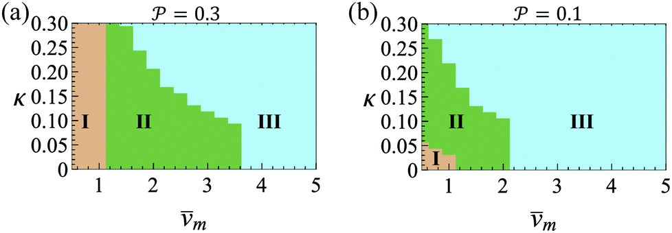 | ||
Fig. 4 State diagram for pushers (a)  and (b) and (b)  . Region I: unstable trajectories that spiral out to result in channel-wide swinging, Region III: stable centerline swimming, Region II: both dynamic states coexist; they depend on the initial condition. Other parameters: Wi = 0.1, ψ0 = 0. . Region I: unstable trajectories that spiral out to result in channel-wide swinging, Region III: stable centerline swimming, Region II: both dynamic states coexist; they depend on the initial condition. Other parameters: Wi = 0.1, ψ0 = 0. | ||
| Type | Lift velocity ∝ Wi | Wall contribution to ẋ |
|---|---|---|
| Passive |
|
— |
| SD | −x(1 + δ)cosψ |
(sinψ)κ3/ε3 |
| FD |
|
|
In conclusion, the current study analyzes microswimmers in weakly viscoelastic pressure-driven flows. For neutral and pusher/puller microswimmers, we derive an additional swimming lift velocity depending on the swimmer's hydrodynamic signature that adds to the passive viscoelastic lift.33,41,60,61 For source-dipole (neutral) swimmers, the swimming lift is two orders of magnitude stronger than the passive lift, which was considered alone in a recent study.33 The current work shows that the swimming lift accelerates the centerline focusing. For force-dipole swimmers (pusher/puller), the swimming lift does not contribute to a net cross-streamline migration. Incorporating hydrodynamic wall interactions, we show that upstream swimming for weak flow strengths qualitatively follows the behavior in Newtonian fluids:11 attraction of pushers towards the channel walls and repulsion of pullers. The downstream swimming along the centerline qualitatively remains the same as that of a passive particle. Finally, we stress that our analysis is valid for an arbitrary swimming direction, which can be decomposed in swimming along and perpendicular to the shear plane.
Interestingly, the results suggest that normal stresses in viscoelastic fluids generated by the flow field of a neutral swimmer can accelerate the centerline focusing. However, this strongly depends on the hydrodynamic signature of the microswimmer. Even for a weakly viscoelastic fluid (Wi = 0.1), we observe rapid focusing within a traveled distance of 10–500 times the channel width (Fig. 2), which amounts to ca. 1–50 mm and is quite realistic for microfluidic channels. Thereby, this work contributes to the understanding of swimming in more realistic biological fluids. We note that higher order multipoles like force quadrupole, rotlet dipole and so on, will have their own  . Therefore, we foresee further development in understanding the trajectories of microswimmers that exhibit higher order multipoles in their hydrodynamic disturbance. Furthermore, the current work offers several new directions to explore. For instance, elongated microswimmers, like passive particles, perform Jeffery orbits in sheared Newtonian fluids.62 In viscoelastic fluids the flow disturbances from swimming will alter the orientation evolution of these orbits and hence the swimmer dynamics.34 The impact of shear-thinning fluids is also an interesting outlook, which can be achieved by the use of more detailed rheological models.46
Conflicts of interest
There are no conflicts to declare.Acknowledgements
Support from the Alexander von Humboldt Foundation is gratefully acknowledged.Notes and references
- S. S. Suarez and A. Pacey, Hum. Reprod. Update, 2006, 12, 23–37 CrossRef CAS PubMed.
- R. Levy, D. B. Hill, M. G. Forest and J. B. Grotberg, Integr. Comp. Biol., 2014, 54, 985–1000 CrossRef CAS PubMed.
- A. Persat, C. D. Nadell, M. K. Kim, F. Ingremeau, A. Siryaporn, K. Drescher, N. S. Wingreen, B. L. Bassler, Z. Gitai and H. A. Stone, Cell, 2015, 161, 988–997 CrossRef CAS.
- J. C. Conrad and R. Poling-Skutvik, Annu. Rev. Chem. Biomol. Eng., 2018, 9, 175–200 CrossRef PubMed.
- M. Jabbarzadeh, Y. Hyon and H. C. Fu, Phys. Rev. E, 2014, 90, 043021 CrossRef PubMed.
- A. E. Patteson, A. Gopinath and P. E. Arratia, Curr. Opin. Colloid Interface Sci., 2016, 100, 86–96 CrossRef.
- J. P. Celli, B. S. Turner, N. H. Afdhal, S. Keates, I. Ghiran, C. P. Kelly, R. H. Ewoldt, G. H. McKinley, P. So and S. Erramilli, et al. , Proc. Natl. Acad. Sci. U. S. A., 2009, 106, 14321–14326 CrossRef CAS PubMed.
- F. Bretherton and N. M. V. Rothschild, Proc. Biol. Sci., 1961, 153, 490–502 Search PubMed.
- J. Hill, O. Kalkanci, J. L. McMurry and H. Koser, Phys. Rev. Lett., 2007, 98, 068101 CrossRef.
- R. Nash, R. Adhikari, J. Tailleur and M. Cates, Phys. Rev. Lett., 2010, 104, 258101 CrossRef CAS PubMed.
- A. Zöttl and H. Stark, Phys. Rev. Lett., 2012, 108, 218104 CrossRef PubMed.
- A. Zöttl and H. Stark, Eur. Phys. J. E, 2013, 36, 1–10 CrossRef PubMed.
- C.-k. Tung, F. Ardon, A. Roy, D. L. Koch, S. S. Suarez and M. Wu, Phys. Rev. Lett., 2015, 114, 108102 CrossRef.
- A. J. Mathijssen, N. Figueroa-Morales, G. Junot, É. Clément, A. Lindner and A. Zöttl, Nat. Comm., 2019, 10, 1–12 CrossRef CAS.
- E. Lauga, The fluid dynamics of cell motility, Cambridge University Press, 2020, vol. 62 Search PubMed.
- E. Lauga, Phys. Fluids, 2007, 19, 083104 CrossRef.
- X. Shen and P. E. Arratia, Phys. Rev. Lett., 2011, 106, 208101 CrossRef CAS PubMed.
- L. Zhu, E. Lauga and L. Brandt, Phys. Fluids, 2012, 24, 051902 CrossRef.
- O. S. Pak, L. Zhu, L. Brandt and E. Lauga, Phys. Fluids, 2012, 24, 103102 CrossRef.
- N. C. Keim, M. Garcia and P. E. Arratia, Phys. Fluids, 2012, 24, 081703 CrossRef.
- G. J. Elfring and E. Lauga, Complex fluids in biological systems, Springer, 2015, pp. 283–317 Search PubMed.
- J. Sznitman and P. E. Arratia, Complex Fluids in Biological Systems, Springer, 2015, pp. 245–281 Search PubMed.
- G. Li and A. M. Ardekani, J. Fluid Mech., 2015, 784, R4 CrossRef.
- C. Datt, L. Zhu, G. J. Elfring and O. S. Pak, J. Fluid Mech., 2015, 784, R1 CrossRef.
- G. Li and A. M. Ardekani, Phys. Rev. Lett., 2016, 117, 118001 CrossRef.
- G. Li and A. M. Ardekani, Eur. J. Comput. Mech., 2017, 26, 44–60 CrossRef.
- T. R. Ives and A. Morozov, Phys. Fluids, 2017, 29, 121612 CrossRef.
- C. Datt, G. Natale, S. G. Hatzikiriakos and G. J. Elfring, J. Fluid Mech., 2017, 823, 675–688 CrossRef CAS.
- Y. Zhang, G. Li and A. M. Ardekani, Phys. Rev. Fluids, 2018, 3, 023101 CrossRef.
- A. Zöttl and J. M. Yeomans, Nat. Phys., 2019, 15, 554–558 Search PubMed.
- A. Choudhary, T. Renganathan and S. Pushpavanam, J. Fluid Mech., 2020, 899, A4 Search PubMed.
- J. P. Binagia, A. Phoa, K. D. Housiadas and E. S. Shaqfeh, J. Fluid Mech., 2020, 900, A4 Search PubMed.
- A. J. Mathijssen, T. N. Shendruk, J. M. Yeomans and A. Doostmohammadi, Phys. Rev. Lett., 2016, 116, 028104 CrossRef PubMed.
- M. De Corato and G. D'Avino, Soft Matter, 2017, 13, 196–211 RSC.
- A. M. Ardekani and E. Gore, Phys. Rev. E, 2012, 85, 056309 CrossRef CAS PubMed.
- A. Zhang, W. L. Murch, J. Einarsson and E. S. Shaqfeh, J. Nonnewton. Fluid Mech., 2020, 104279 CrossRef CAS.
- A. P. Berke, L. Turner, H. C. Berg and E. Lauga, Phys. Rev. Lett., 2008, 101, 038102 CrossRef PubMed.
- D. Smith, E. Gaffney, J. Blake and J. Kirkman-Brown, J. Fluid Mech., 2009, 621, 289–320 CrossRef.
- A. Karnis and S. Mason, J. Rheol., 1966, 10, 571–592 CAS.
- F. Gauthier, H. Goldsmith and S. Mason, J. Rheol., 1971, 15, 297–330 CAS.
- B. Ho and L. Leal, J. Fluid Mech., 1976, 76, 783–799 CrossRef.
- D. Li and X. Xuan, Phys. Rev. Fluids, 2018, 3, 074202 CrossRef.
- A. Choudhary, D. Li, T. Renganathan, X. Xuan and S. Pushpavanam, J. Fluid Mech., 2020, 898, A20 CrossRef CAS.
- A. Choudhary, T. Renganathan and S. Pushpavanam, Phys. Rev. Fluids, 2021, 6, 036701 CrossRef.
- L. Leal, J. Nonnewton. Fluid Mech., 1979, 5, 33–78 CrossRef CAS.
- R. B. Bird, C. F. Curtiss, R. C. Armstrong and O. Hassager, Dynamics of polymeric liquids, fluid mechanics, Wiley, 1987, vol. 1 Search PubMed.
- B. Caswell and W. Schwarz, J. Fluid Mech., 1962, 13, 417–426 CrossRef.
- L. Leal, J. Fluid Mech., 1975, 69, 305–337 CrossRef.
- D. L. Koch and G. Subramanian, J. Nonnewton. Fluid Mech., 2006, 138, 87–97 CrossRef CAS.
- M. Lighthill, Commun. Pure Appl. Math., 1952, 5, 109–118 CrossRef.
- J. R. Blake, J. Fluid Mech., 1971, 46, 199–208 CrossRef.
- A. Zöttl and H. Stark, J. Phys.: Condens. Matter, 2016, 28, 253001 CrossRef.
- H. Lamb, Hydrodynamics, Cambridge, Cambridge University Press, 6th edn, 1975 Search PubMed.
- T. Pedley and J. O. Kessler, Annu. Rev. Fluid Mech., 1992, 24, 313–358 CrossRef.
- K. Drescher, R. E. Goldstein, N. Michel, M. Polin and I. Tuval, Phys. Rev. Lett., 2010, 105, 168101 CrossRef PubMed.
- K. Drescher, J. Dunkel, L. H. Cisneros, S. Ganguly and R. E. Goldstein, Proc. Natl. Acad. Sci. U. S. A., 2011, 108, 10940–10945 CrossRef CAS PubMed.
- S. Chattopadhyay, R. Moldovan, C. Yeung and X. Wu, Proc. Natl. Acad. Sci. U. S. A., 2006, 103, 13712–13717 CrossRef CAS PubMed.
- I. Minoura and R. Kamiya, Cell Motil. Cytoskeleton, 1995, 31, 130–139 CrossRef CAS PubMed.
- S. E. Spagnolie and E. Lauga, J. Fluid Mech., 2012, 700, 105–147 CrossRef.
- E. F. Lee, D. L. Koch and Y. L. Joo, J. Nonnewton. Fluid Mech., 2010, 165, 1309–1327 CrossRef CAS.
- G. D'Avino, F. Greco and P. L. Maffettone, Ann. Rev. Fluid Mech., 2017, 49, 341–360 CrossRef.
- G. B. Jeffery, Proc. Math. Phys. Eng., 1922, 102, 161–179 Search PubMed.
Footnotes |
| † Electronic supplementary information (ESI) available. See DOI: 10.1039/d1sm01339d |
| ‡ The correction to the drift velocity in z-direction is −Wixκsinψ(1 + δ), and the correction to rotation is found to be −2Wiκsinψ. We verified that these modifications do not qualitatively alter the dynamics and thus neglect their contributions for simplicity. Details are provided in the ESI.† |
| This journal is © The Royal Society of Chemistry 2022 |