
 Open Access Article
 This Open Access Article is licensed under a
 Creative Commons Attribution 3.0 Unported Licence
Towards time resolved characterization of electrochemical reactions: electrochemically-induced Raman spectroscopy†
Luca
D'Amario
 *ab,
Maria Bruna
Stella
c,
Tomas
Edvinsson
d,
Maurizio
Persico
c,
Johannes
Messinger
ae and
Holger
Dau
b
*ab,
Maria Bruna
Stella
c,
Tomas
Edvinsson
d,
Maurizio
Persico
c,
Johannes
Messinger
ae and
Holger
Dau
b
aDepartment of Chemistry, Ångström Laboratory, Uppsala University, Box 523, 751 20 Uppsala, Sweden. E-mail: luca.damario@kemi.uu.se; Fax: +46 18 471 6844; Tel: +46 18 471 6584
bDepartment of Physics, Freie Universität Berlin, Arnimallee 14, 14195 Berlin, Germany
cDepartment of Chemistry and Industrial Chemistry, University of Pisa, Via Moruzzi 13, 56124 Pisa, Italy
dDepartment of Materials Science and Engineering, Uppsala University, Box 35, 751 03 Uppsala, Sweden
eDepartment of Chemistry, Chemical Biological Centre, Umeå University, 90187 Umeå, Sweden
First published on 30th August 2022
Abstract
Structural characterization of transient electrochemical species in the sub-millisecond time scale is the all-time wish of any electrochemist. Presently, common time resolution of structural spectro-electrochemical methods is about 0.1 seconds. Herein, a transient spectro-electrochemical Raman setup of easy implementation is described which allows sub-ms time resolution. The technique studies electrochemical processes by initiating the reaction with an electric potential (or current) pulse and analyses the product with a synchronized laser pulse of the modified Raman spectrometer. The approach was validated by studying a known redox driven isomerization of a Ru-based molecular switch grafted, as monolayer, on a SERS active Au microelectrode. Density-functional-theory calculations confirmed the spectral assignments to sub-ms transient species. This study paves the way to a new generation of time-resolved spectro-electrochemical techniques which will be of fundamental help in the development of next generation electrolizers, fuel cells and batteries.
1 Introduction
One of the most fundamental goals of modern chemistry is to investigate reaction mechanisms down to their most elemental steps. In this regard, since its first application in the 50's, time resolved spectroscopy has been crucial in elucidating processes as diverse as vision, natural photosynthesis, electron transfer, DNA damage, heat transfer and quantum computing.1–11 In a typical time resolved spectroscopy measurement, the sample is excited with a pulse of light and the changes in its spectroscopic signal are monitored in time.12 To be able to perform such measurements the initial step of the studied process has to be photo-induceable.13–15 This is a limitation as the reaction under study might not be photochemical, or the sample not transparent. In addition, for chemical processes occurring as rare events, ultrafast transient spectroscopies have limited use, instead detailed spectroscopic information on species formed under micro- or millisecond time scales are preferred.Electrochemical (e-chem) reactions are of great importance in modern technology, for example they are key to the functioning of batteries, electronic components, industrial production, electrolyzers and fuel cells.16–19 Despite their widespread use, the mechanisms of these reactions are difficult to study at fast time scales, i.e. by classical time resolved spectroscopy, because these reactions cannot or should not be photo-induced. Presently, chemico-physical information on e-chem processes are instead acquired, aside from electrochemistry, via in situ spectroscopic techniques, such as UV-vis spectroelectrochemistry, in situ Raman, IR and X-ray spectroscopy.20–28 In such methods an electrochemical cell is constructed such that a spectroscopic signal can be read from the surface of the electrode; the signal is measured while a given potential is applied. Usually, in these experiments, when the signal is recorded, the system is in a steady state; e.g. the measurement starts after a stable current reading is reached. In this way, no information on dynamics can be extracted. The signal originates from the average composition of the system at that given potential, i.e. from stable species. Thus, information on fast reacting species, in the ms time scale and faster, are lacking. This, generally speaking, hinders the understanding and development of e-chem processes and related devices; a classic example is the missing description of the dynamics of the lithium ion intercalation on Li-battery anodes.
Attempts to achieve time resolution with in situ techniques have been made.29–32 Commonly, a potential step is applied to trigger the e-chem reaction, while a series of spectra are recorded with short detector sampling time.33–37 With this strategy the speed of the detector is a crucial and limiting factor to time resolution. Moreover, limitations can also arise from a large time constant of the electrochemical cell.37 Among the techniques listed above, Raman spectroscopy is recently gaining popularity due to the simplicity of in situ implementation, its ability to give structural information and “high” time resolution. Common detectors, e.g. charge-coupled-device (CCD) cameras, have shortest sampling time of merely ca. 100 ms. This is a timescale of ion diffusion/migration, or macroscopic structural rearrangements like bubble formation. To be able to study reaction mechanism (bond breaking/formation) or ion exchange/intercalation or molecular structural rearrangements, time resolution of at least 0.1–0.01 ms is needed. Such a fast detection would require an upgrade to a purposely faster device, which however is expensive and not always possible. To the best of our knowledge, there is only one example of an in situ Raman setup (and in situ in general) that was equipped with a gated CCD camera that could reach 10–100 ms time resolution, by sampling the light only during short selected time periods.35 The downsides to this approach are, firstly, a low signal-to-noise ratio (S/N) necessitating extensive data collection, and secondly, the full potential of the camera (10–100 ns gating) cannot be utilized because the slow read-out limits its time resolution.
In this paper, simple (and unexpensive) modifications to a commercial confocal Raman spectrometer are reported that allow synchronisation of the Raman signal detection with the application of an electric pulse. The variation of the time period of this electric pulse allows to resolve transient intermediates, down to a maximum time resolution achieved presently of 0.6 ms. This is about 100 times faster than what was reached previously with an e-chem in situ structural spectroscopic method.34,35 As a test of the technique, a known electrochemical reaction is studied.
2 Results and discussion
2.1 Technique description
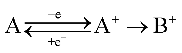
To be able to describe the working principles of the new technique presented here, the Electrochemical Induced Raman spectroscopy (EIR), it is useful to refer to a hypothetical electrochemical model. In the following, an irreversible EC system (electron transfer, followed by a chemical reaction) is considered:here a species A can be oxidized to the unstable species A+ which can convert to the stable species B+. A hypothetical CV of such system is reported in Fig. 1, showing a slow scan-rate experiment (solid line) and a fast one (added dashed line). Here “slow” and “fast” are taken in respect to the A+ → B+ reaction. It should be noted that, for clarity purposes, in Fig. 1 an “infinite pool” of the A species is assumed (e.g. reversible or diffusion controlled or catalytic systems), which assures the repeatability of the electrochemical cycle.
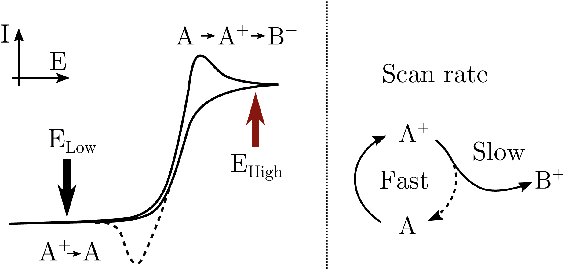 | ||
| Fig. 1 Schematic cyclic voltammogram of the A/A+/B+ system described in the text, in dashed lines the response obtained at scan-rates able to outcompete reaction A+ → B+. An “infinite pool” of the A species is assumed. On the right, the reaction scheme in function of scan-rates, fast vs. slow. | ||
As shown in Fig. 1, in the slow scan, only an irreversible oxidation wave is present (with no reduction), while in the fast scan the potential sweep is fast enough to compete with the A+ → B+ conversion allowing the reduction of the A+ species. This system could be studied with classical in situ techniques, comparing spectra collected at two different potentials, Elow and Ehigh, see Fig. 1. In such a hypothetical study, only the two stable species A and B+ would be observed, due to relative low concentration of the transient species in the steady-state conditions. In this example, the goal of the technique presented in this paper, would be to detect the unstable species A+.
The strategy adopted here is to apply a potential pulse of a given time period and amplitude to produce the wanted elusive state, say A+, and probe the system, via spectroscopy, only in this time period.
In practice, pumping is achieved by applying a train of potential pulses to an electrode (in an e-chem cell), i.e. a potential square wave (SW), see scheme in Fig. 2. The SW can be described by its frequency (ω), amplitude (A), phase (ϕ) and offset (E0) (potential bias). For practical reason, in the following discussion instead of amplitude and offset, the parameters “high” and “low” potentials will be used, respectively Ehigh and Elow, see Fig. 2.
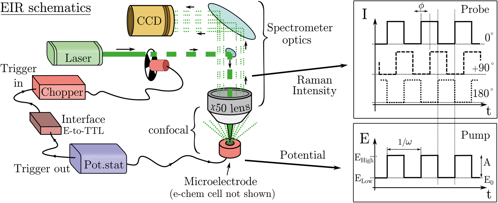 | ||
| Fig. 2 Scheme of the EIR setup with example of the modulation of Raman intensity and potential vs. time. Only the parts shown in RED are added to a usual Raman spectrometer to implement EIR. In the graphs, ϕ indicates the possibility to shift the phase of the Raman modulation (0°/90°/180°) with respect to the potential SW. | ||
The electrode surface, where the reaction occurs, is placed in the focus of a Raman spectrometer (in microscope/confocal configuration) so that the Raman scattering coming from the surface of the electrode can be collected and analysed. The Raman laser intensity is also modulated at the same frequency of the potential modulation and is phase synchronised by a mechanical chopper, see Fig. 2. In this way the light that reaches the detector (CCD camera) is only the one that interacts with the sample in the desired pump SW state. Indeed, by changing the phase synchronisation, the Raman spectrometer can probe either the “high” potential (0° phase shift) or the “low” potential (180° phase shift) of the SW, see schemes in Fig. 2. The spectra of the high and low potential pulse state will be denoted H and L, respectively. The transient signal is given by the difference with a reference Raman spectrum (ref, which typically is the spectrum of the system without potential bias), Hr = H − ref. In the case of constant reaction rates during both the high and low crests of the SW, the 0/180° delta Raman, might not be informative due to similar average compositions. In these cases spectra recorded at ±90°, which probes the rising (R, −90°) or the falling (F, +90°) edge of the SW, are the most descriptive cases, see Fig. 2 and S3 in ESI.†
The periodic nature of the pump requires that the system in study should be able to restore, at least partially, to its initial condition at every period.
The formation or breaking of a bond can be visible in the Raman signal which can provide structural information of the species that are evolving between the high and low state of the SW, see Fig. 3. In particular, fast evolving phenomena will be more visible in the spectra recorded at high SW frequencies (short pump/probe pulses) in respect to the slow phenomena that will be visible at any frequency, see Fig. 3.
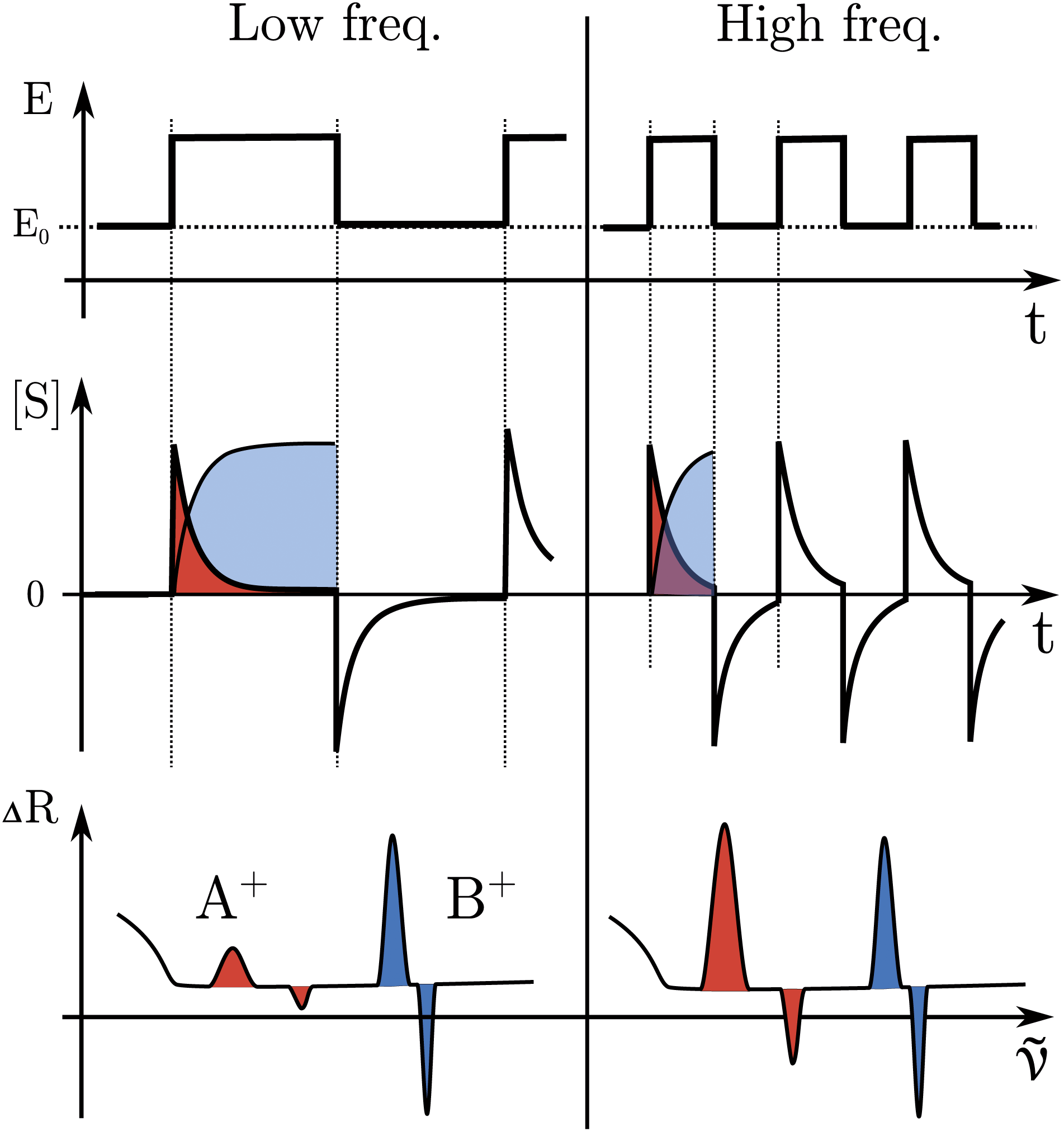 | ||
| Fig. 3 Expected data from an EIR measurement; comparison between low and high frequency results. In the top, the pump SW; in the middle, the evolution of the species concentration; in the bottom, the Raman difference spectra. Areas in red represent the signal from a fast evolving state, those in blue a slowly evolving or stable one. | ||
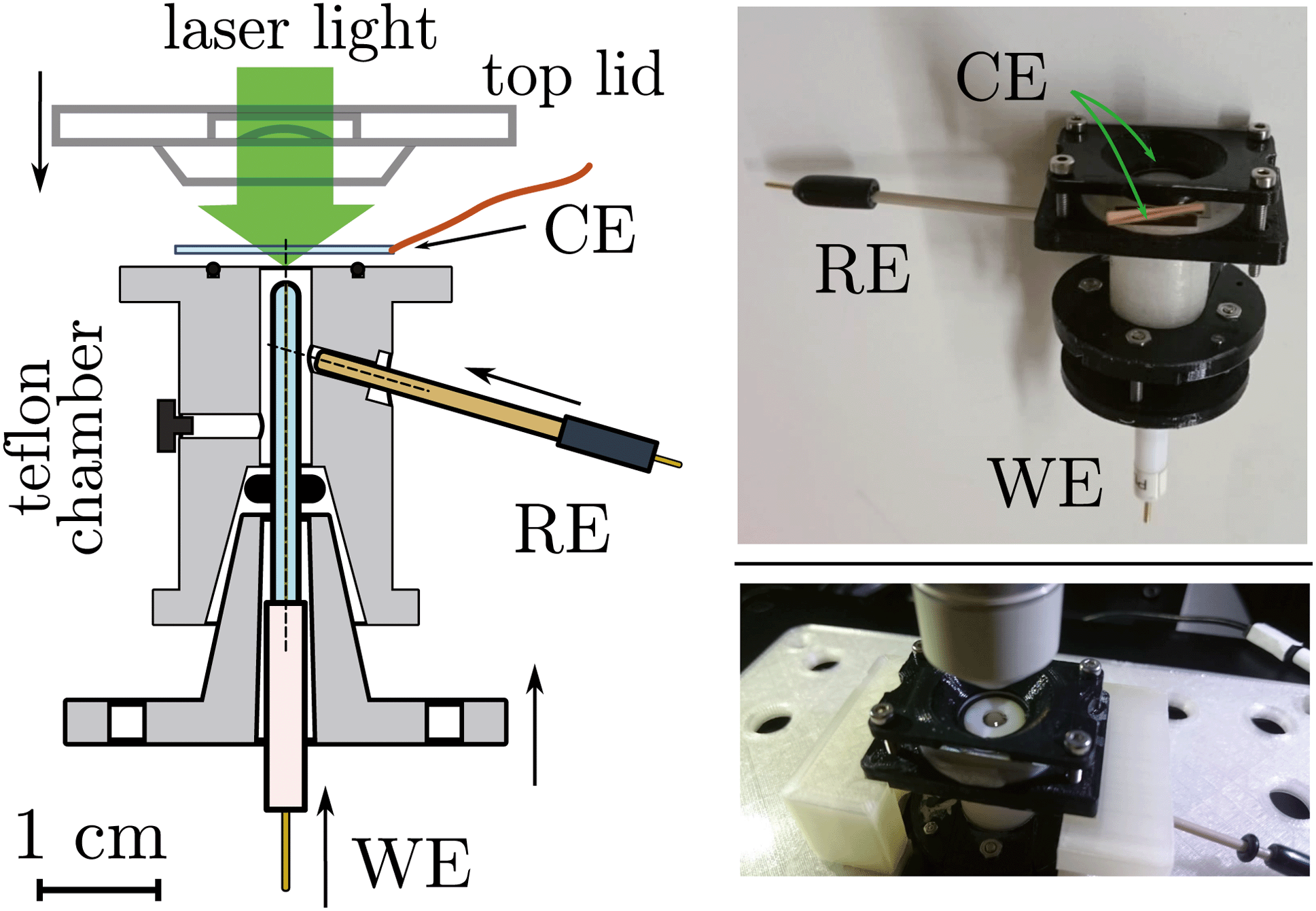 | ||
| Fig. 4 (Left) Section of the e-chem cell design (Teflon made), see Fig. S1 in ESI,† for detailed technical sketches. The WE and RE electrodes are shown in the final positions, for clarity the CE is not attached to the cell. Supporting flanges for closure are not shown. (Right) Pictures of the real cell. | ||
A light chopper can be easily placed in the laser path in any position before the beam enters the spectrometer and also be used for any of the lasers installed in the Raman set-up. The chopper controller can be synchronised (in frequency and phase) with the potentiostat, see Fig. 2. The Raman signal probes similar time scales of the width of the potential pulse, thus the time resolution is limited to the shortest period of the SW/Raman modulation. In this regard, the possibility to use instead (ns) pulsed lasers was discarded since many of these systems can mode lock differently in between the pulses, which causes several nanometers shift of the laser emission band; this, disqualifies them for use as a Raman laser which requires a highly monchromatic and stable laser line.
2.2 Validation
A known Ru based molecular switch, RuN6, see Fig. 5, was selected to test the EIR technique.38–40 This system was chosen due to its rare combination of characteristics: it is reversible and highly stable, with a known reaction mechanism and desired kinetics (ca. 200 s−1).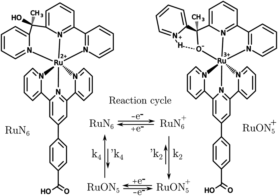 | ||
| Fig. 5 Structures of RuN6, [Ru(HOOC–Ph-tpy)(1-[6-(2,2′-bipyridyl)]-1-(2-pyridyl)ethanol)]2+, and RuON5+ with related reaction cycle of the electron transfer induced isomerization. k2 and k4 are ca. 150–200 and 500–1000 s−1, respectively (e− transfers occur in ca. 104 s).39 | ||
RuN6 is a hexapyridyl coordinated Ru(II) complex that shows structural bistability depending on the Ru center oxidation state. The switching ligand, here abbreviated “BpyPyEt”, favores an N bond to Ru(II) while it binds via O to Ru(III); the full isomerization cycle is shown in Fig. 5. The isomerization can be followed by microelectrode cyclic voltammetry at different scan rates, see Fig. 6 and S4.† At low scan rates the CV shows an irreversible redox behaviour originating from the two stable species RuN6 and RuON5+; while at fast scan rates, where the reverse redox reaction competes efficiently with the isomerization, the CV shows two reversible redox couples, i.e. all the four species (see ESI† for a detailed treatment supported by e-chem data).
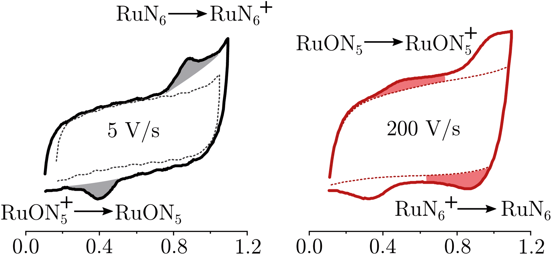 | ||
| Fig. 6 Electrochemistry of RuN6 grafted on Pt microelectrode, at two scan-rates 5 and 200 V s−1. In dashed lines the blank electrochemistry (without complex) to account for the coulombic current. The grey areas indicate the irreversible waves due to the stable species; the red areas indicates the redox waves due to the unstable species, visible only at high scan-rates. | ||
Lomoth et al. have shown that the isomerization kinetics can be tuned by changing the alkyl substituent of the bridging carbon of the pyridil-C-bipyridil ligand.39 With the methyl substituent used here, the RuN6 shows a kinetics of about 200 s−1 which is on the timescale reachable by the EIR, but hardly by any other spectroelectrochemical technique. Indeed, the isomerization mechanism has been proven only via electrochemical methods supported by computational simulations. We emphasize that in the EIR experiment, not only does the basic Raman-scattering detection scheme provide high time resolution, but also the spatial resolution is on the order of few micrometers, allowing the use of microelectrodes that support sub-microsecond electrochemical response times. Here we can directly probe the isomerization by Raman spectroscopy, thereby illustrating the potential of the new EIR methodology. Namely, at low pump SW frequencies, only the stable RuN6 and RuON5+ spectra should be visible in the spectra, while at high frequencies the transient species RuN6+ and RuON5, should also appear.
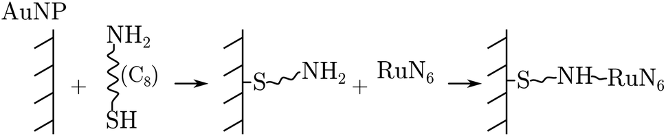
RuN6 was loaded on a (Φ = 100 μm) gold electrode functionalized with gold nanoparticles (AuNP) to enable surface-enhanced Raman spectroscopy (SERS). Linkage occurred through amino-thiol chains, as the following reaction sequence summarizes:
This results in a monolayer coverage of the electrode area. A purposely designed Raman imaging measurement of the functionalised electrode was carried out to localize enhancement hotspots (see ESI†); which revealed that the majority of the hotspots are located at the edge of the microelectrode. EIR spectra were then collected using a slightly defocused beam spot (to increase its size) placed at the edge of the electrode, see the ESI† for further details.
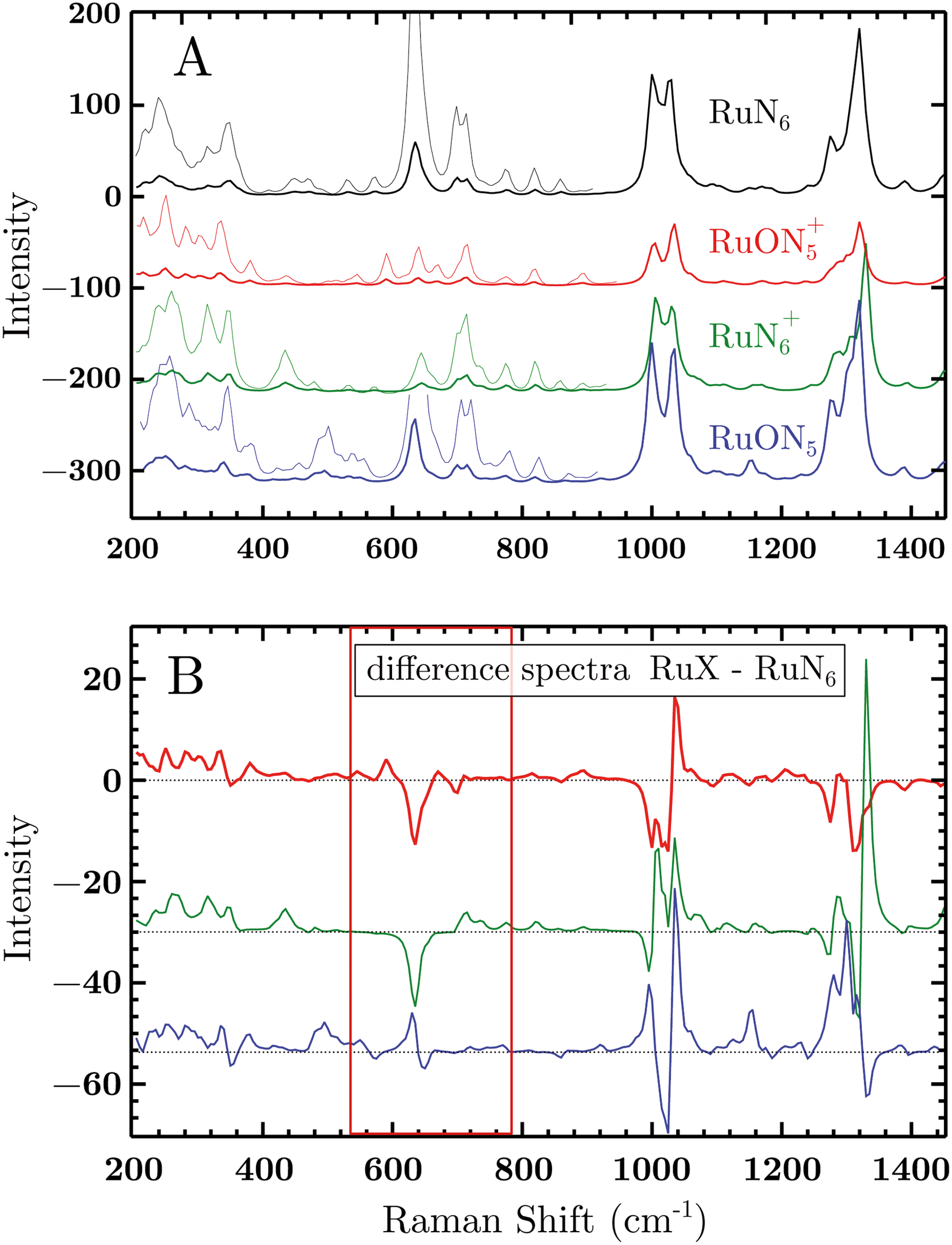 | ||
| Fig. 7 (A) Vibrational Raman spectra of the RuN6 family calculated by DFT. The spectra were produced by a sum of Lorentzian functions (15 cm−1 FWHM) constructed from the frequencies and amplitudes of the simulated modes. The intensities in the region 150–800 cm−1 were magnified ×5 for clarity. (B) Difference spectra calculated from above data subtracting the RuN6 spectrum from the other three. The spectral range of main interest has been highlighted. The spectra are offset for clarity. | ||
To test the accuracy of these calculations we compared the RuN6 DFT spectrum with the experimental powder spectrum (Fig. S10†). These agree within ±30 cm−1, which is sufficient for our scope. We additionally analyzed the effect of H/D substitution (Fig. S10†), which confirms that relevant peaks, for species discrimination, can be found at 600–750 cm−1, 1000 cm−1 and around 1300 cm−1.
Based on electrochemical kinetics analysis and taking RuN6 as reference (the stable species at open circuit potential, ocp), a rough estimation of the experimental difference spectra can be performed. Considering that the maximum EIR pump semiperiod is 0.6 ms and that the isomerization constants are 150–200 s−1 and 500–1000 s−1, for k2 and k4 respectively, it can be predicted that the transient RuN6+ species (green spectrum in Fig. 7A) should be observed, while the RuON5 isomer (blue spectrum) might not be. In order to emulate the EIR difference spectra, the calculated RuN6 spectrum has been subtracted from the spectra of the other three species to produce the difference spectra in Fig. 7B. Following the predictions just listed, the difference spectra at mid-low pump frequency should resemble the RuON5+–RuN6 (red) spectrum in Fig. 7B (e.g. with mainly negative features around 650, 1050 and 1300 cm−1); while at fast pump frequencies, new difference (positive) features should appear at around 710, 1000, 1300 cm−1, resembling the RuN6+–RuN6 (green) spectrum in Fig. 7B.
The DFT calculated spectra have been used to perform a numerical simulation of the EIR difference spectra in order to accurately predict the experimental results. The simulation was carried out operating a weighted integration of the kinetics laws of all the evolving species to calculate every contribution in each EIR spectrum. The weighting law resembles the shape of the probe pulse train. The full simulation is reported in the ESI.† Here only the one relevant spectrum is shown, the 834 − Rr difference spectrum (which is similar to the Hr and Rr, see Fig. S21†), reported in comparison to the experimental data, in Fig. 8. It can be seen that the 834-Rr simulated spectrum, i.e. the Rr spectrum at the highest time resolution, indeed resembles the RuN6+–RuN6 green spectrum in Fig. 7B, as intuitively predicted above.
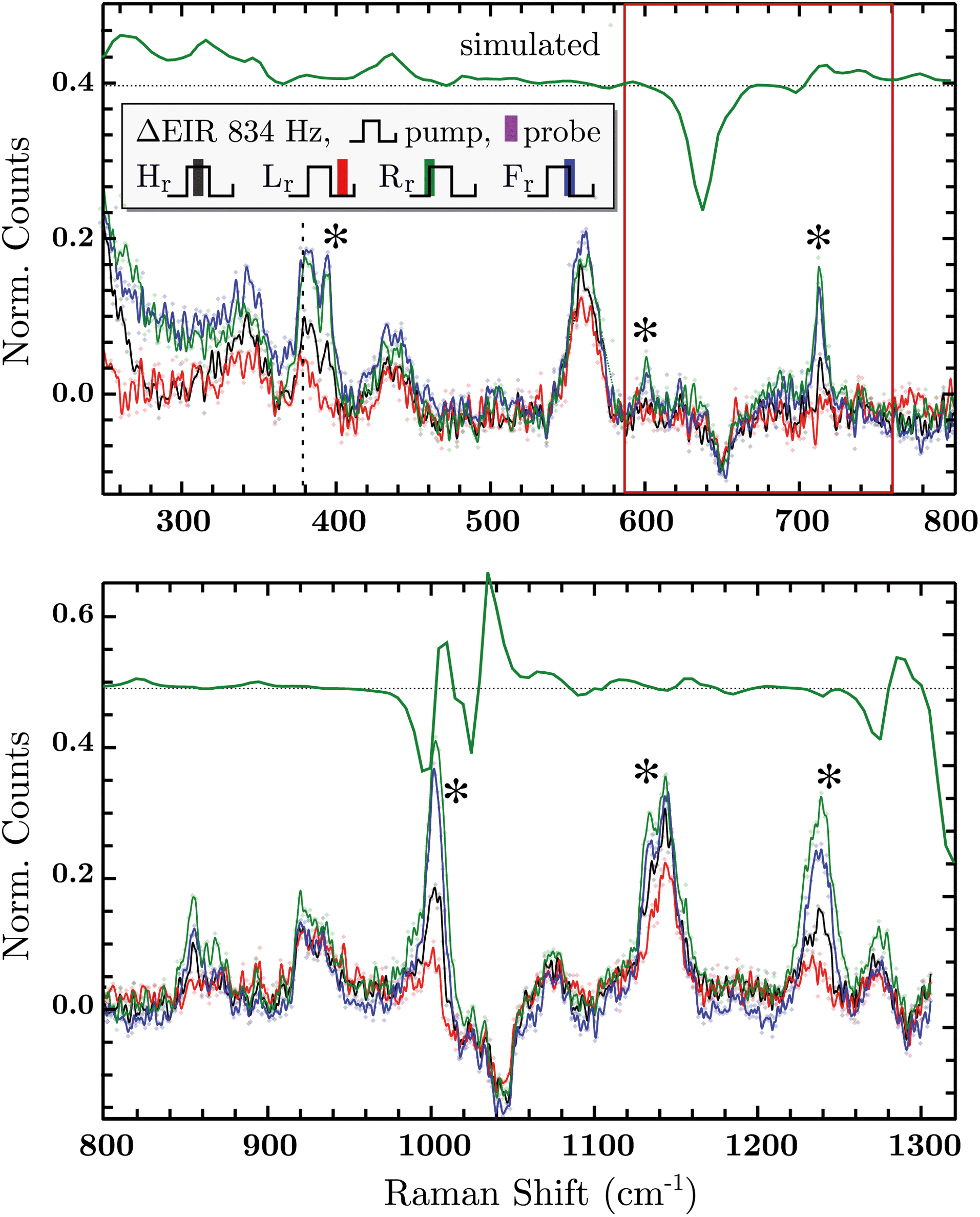 | ||
| Fig. 8 Difference EIR spectra of the RuN6 functionalised AuNP electrode of the 834 Hz measurement in all four phase shifts, the ocp spectrum has been taken as reference (subtracted and normalized). EIR phases: Hr black, Lr red, Rr green, Fr blue. The Rr trace from numerical simulation is reported in green, shifted for clarity. Discussed spectral range has been highlighted for clarity. | ||
Delta EIR spectra have been calculated, by treating the raw spectra according to literature protocols, to account for a different magnitude of enhancement.41 Briefly, the flat background B is subtracted from the raw spectra R and is also used to normalize them, the final spectra being S = (R − B)/B. The spectrum recorded at ocp (reported in Fig. S16†) has been taken as reference which was subtracted from the 20 − H (spectrum recorder at 20 Hz pump frequency, “high” phase) and 834 − H spectra producing the results reported in the ESI, Fig. S17.† Here we report only the most significant difference spectra, i.e. all phases Hr/Lr/Rr/Fr, recorded at the fastest pumping frequency, 834 Hz, in Fig. 8.
In Fig. 8, negative difference bands can be found: at 650 cm−1; a broad band at 1050 cm−1; and a final at ca. 1300 cm−1. These negative features derive from the subtraction with the ocp spectrum that was taken as reference, see Fig. S16.† Relevant positive difference bands (indicated with asterisks) are found at: 392; 600; 712; 1000; 1140 and 1230 cm−1. Other positive bands are of less interest since they are present in all EIR difference spectra of all pumping frequencies, again derived from differences with the ocp spectrum. These omnipresent positive and negative bands are likely due to slowly evolving transient species (i.e. species that appear/disappear only on a fully rested system, at ocp). This is supported by the electrochemical kinetic measurements, which show a small, slow (6.7 s−1) component in the isomerization kinetics, see ESI† for further details.
As predicted, the 834 − Hr spectrum resembles the 20 − Hr spectrum, see Fig. S17,† meaning it does not display clear transient features. Transient bands can be seen in the ±90° (Rr and Fr, green and blue respectively), that are not present or are not as strong in the 0/180° (Hr and Lr, black and red). This is expected since, as mentioned earlier, depending on conditions, the ±90° phase spectra can probe faster evolving processes, vide infra.
The experimental delta spectra, in Fig. 8, are expected to be a combination of all the four species. This is due in part to the kinetics of the system and in part to the not perfectly squared shape of the probe pulses. The pulses show a rising/falling components that mix the H and L signals around the edges, see ESI† for a thorough clarification regarding this topic. Indeed, it can be seen that each of the EIR spectra contains features of the calculated spectra in Fig. 7. However, it is also clear that the new features that arise in the ±90° spectra resemble mainly the RuN6+–RuN6 (green) difference spectrum in Fig. 7B, as well as the simulated 834 − Rr spectrum in Fig. 8, with remarkable accuracy in the 250–800 cm−1 region. In Fig. 8, a sharp positive feature, at 712 cm−1, absent in the Lr difference spectrum, is present with medium intensity in the Hr spectrum and quite prominent in the Rr and Rr difference spectra. In the same region, a broad negative band at around 650 cm−1 and a small positive peak at 600 cm−1 can be observed. Altogether these three peaks can be constructed by the sum of the computed different spectra, red, green and blue in Fig. 7, with prevalence of the green spectrum. Overall this leads to assign the 712 cm−1 peak to transient species. Even though the 712 cm−1 peak can be attributed to both unstable isomers, RuN6+ and RuON5 (this last one with weaker amplitude, see Fig. S19†), they are both transient intermediates visible only at sub-ms timescales, proving the effectiveness of the EIR technique.
Other parts of the spectrum, e.g. below 400 cm−1 or around 1000 or 1300 cm−1 are more fluctuating or similar among the species to be considered here, they are discussed in detail in the ESI.†
So far the spectra have been analyzed regarding informative spectral features, though the EIR technique can also give kinetic information (rate constants) by peak magnitude vs. pump frequency analysis. A mathematical model able to deconvolute EIR spectra on the basis of kinetic laws is under development. Here, a simple comparison of single spectra with the predicted kinetics can be performed. The peak at 712 cm−1 has been taken as example for comparison with known kinetic data. The normalized amplitude (vs. the 670–690 cm−1 band, raw spectra) of the 712 cm−1 peak is plotted in Fig. 9 as a function of pump semiperiod, together with the expected kinetic trace from a first order reaction with 200 s−1 rate constant. The results confirm that the experimental findings can be described by the reaction-kinetic model described in Fig. 9.
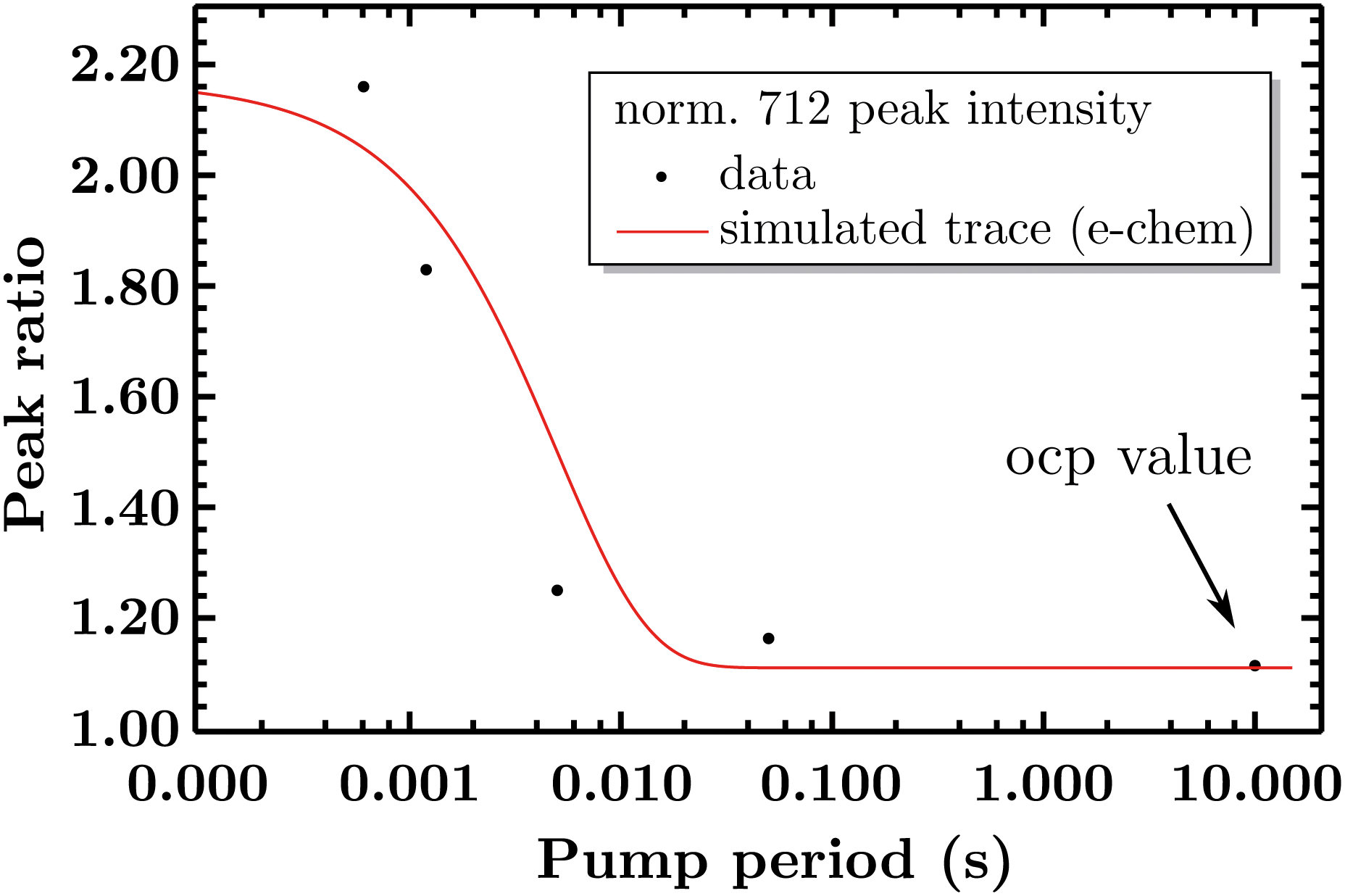 | ||
| Fig. 9 Comparison of the experimental amplitude ratio of the normalized 712 peaks over time and its simulated trace (as a first order reaction) of the measured kinetics (200 s−1). | ||
• The electrode area should be small to ensure fast pump potential response.
• Any electrode material can be used provided having enough scattering from the sample. SERS inactive substrates have been tested and promising preliminary results were obtained with solid inorganic layers (like Co oxides for Li-batteries).
• For reactions involving gas evolution (e.g. water oxidation) a flow cell is needed to remove bubbles from the electrode.
• Spectral simulation is not strictly necessary to interpret EIR results if experimental reference spectra are available or the EIR spectra are simple enough to be interpreted via isotope substitution or fundamental frequency estimation.
3 Conclusion
This report describes and demonstrates the validity of EIR technique, which is the first to combine structural spectroscopy with a pulsed electrochemical protocol achieving sub millisecond time resolution. This enables the effective detection of electrochemical reaction intermediates. We expect this new technique to have a large impact, because of its straight forward adaptation to a large number of important research fields, including batteries and electrocatalysis for renewable energy and circular economy.4 Experimental details
Fast electrochemistry was performed with an Autolab PGSTAT302N equipped with a Scangen and DAC750 modules for fast analog-to-digital conversion. Working microelectrodes for fast e-chem were prepared in-house from Pt or Au wire (50 or 100 μm diameter) and borosilicate glass capillary. Alumina, 0.3 and 0.05 μm diameter, was used to fine polish the metal surface. A graphite rod was used as counter electrode and a Ag wire in a 10 mM AgNO3 solution as reference electrode.Au nanoparticles were synthesized by negatively polarizing a clean surface Au microelectrode, with −0.17 V, in a solution of HAuCl4 0.1 M, in a two electrode cell, for a period of time (typically 5 s), repeated 5 times. Such microelectrode was electrochemically polished by applying, in a two electrode cell, ten cycles between −0.4 and 1.4 V in a 0.5 M H2SO4 solution. The electrode was rinsed with DI water (>18 MΩ cm−1), immersed in a 5 mM solution of 8-amino-octanthiol (8AT) for 30 min, the 8AT functionalized electrode was rinsed and immersed in a solution of the Ru-complex, 5 mM, and 10 mM 4-(4,6-dimethoxy-1,3,5-triazin-2-yl)-4-methylmorpholinium chloride (DTDMM) catalyst for ca. 48 h.
Raman spectroscopy was performed with an inVia spectrometer by Renishaw equipped with three lasers, 473 nm, 532 nm, 785 nm. The 50× objective from Leica was used in the recording of dry samples while a 63× water immersion objective from Leica was used in the EIR and in situ measurements. The phase locked chopper was purchased from Thorlabs (MC2000B); the TTL interface was programmed via a NI MyRIO-1900. Further details are reported in the text and ESI.†
Raman spectra simulations were performed on the optimized molecular geometries. Density Functional Theory (DFT) was employed for the electronic calculations, using the B3LYP exchange–correlation functional.42 The ‘Los Alamos National Labs' effective core potentials were used for the Ru atom.43 The basis set was of double-ζ type (LANL2DZ)43,44 with the addition of polarization functions on the heavy atoms.43,45,46 Solvation effects were included by means of the polarizable continuum model (PCM). For more details, see ESI.†
Details on used materials and compounds are reported in the ESI.†
Data availability
All relevant data is presented either in the article or as in the ESI.† The original data in form of text files can be provided by the corresponding author upon reasonable request.Author contributions
The EIR technique was conceived, designed and implemented by LD. Experiments were performed and analyzed by LD with support of MBS and TE. DFT calculations were performed by MBS and MP. The manuscript was written by LD, JM and HD, with contributions from TE, MBS and MP.Conflicts of interest
The authors declare no coflict of interest.Acknowledgements
The authors are grateful for financial support to the Swedish Research Council, Vetenskaprådet, grant no. 2019-00663, the Alexander von Humboldt Foundation and the Erasmus+ program. The authors thank Reiner Lomoth for useful discussion and for providing the RuN6 sample.Notes and references
- G.-N. Porter, Proc. R. Soc. London, Ser. A, 1950, 200, 284–300 CAS.
- G. Porter and F. J. Wright, Discuss. Faraday Soc., 1953, 14, 23–34 RSC.
- E. Fujimori and R. Livingston, Nature, 1957, 180, 1036–1038 CrossRef CAS.
- V. J. Wulff, R. G. Adams, H. Linschitz and E. Abrahamson, Ann. N. Y. Acad. Sci., 1958, 74, 281–290 CrossRef CAS PubMed.
- R. A. Cone and W. H. Cobbs, Nature, 1969, 221, 820–822 CrossRef CAS PubMed.
- K. Kaufmann, P. Dutton, T. Netzel, J. Leigh and P. Rentzepis, Science, 1975, 188, 1301–1304 CrossRef CAS PubMed.
- T. Melvin, S. Botchway, A. Parker and P. O'Neill, J. Chem. Soc., Chem. Commun., 1995, 653–654 RSC.
- E. Stemp, M. Arkin and J. Barton, J. Am. Chem. Soc., 1997, 119, 2921–2925 CrossRef CAS.
- M. Haumann, P. Liebisch, C. Müller, M. Barra, M. Grabolle and H. Dau, Science, 2005, 310, 1019–1021 CrossRef CAS PubMed.
- K. Ramasesha, L. De Marco, A. Mandal and A. Tokmakoff, Nat. Chem., 2013, 5, 935–940 CrossRef CAS PubMed.
- D. Riste, M. Dukalski, C. Watson, G. De Lange, M. Tiggelman, Y. M. Blanter, K. W. Lehnert, R. Schouten and L. DiCarlo, Nature, 2013, 502, 350–354 CrossRef CAS PubMed.
- T. Weinacht and B. J. Pearson, Time-resolved spectroscopy: An experimental perspective, CRC Press, 2018 Search PubMed.
- G. L. Closs and J. R. Miller, Science, 1988, 240, 440–447 CrossRef CAS PubMed.
- S. Tazuke and N. Kitamura, J. Chem. Soc., Chem. Commun., 1977, 515–516 RSC.
- D. Rehm and A. Weller, Isr. J. Chem., 1970, 8, 259–271 CrossRef CAS.
- J. Tarascon and P. Simon, Electrochemical Energy Storage, Wiley, 2015 Search PubMed.
- J. McHardy and F. Ludwig, Electrochemistry of Semiconductors and Electronics: Processes and Devices, Elsevier Science, 1992 Search PubMed.
- D. Pletcher and F. Walsh, Industrial Electrochemistry, Springer, Netherlands, 2012 Search PubMed.
- M. Breiter, Electrochemical Processes in Fuel Cells, Springer, Berlin, Heidelberg, 2012 Search PubMed.
- K. Adarsh, N. Chandrasekaran and V. Chakrapani, Front. Chem., 2020, 8, 137 CrossRef CAS PubMed.
- J. Wandt, C. Marino, H. A. Gasteiger, P. Jakes, R.-A. Eichel and J. Granwehr, Energy Environ. Sci., 2015, 8, 1358–1367 RSC.
- R. Kas, O. Ayemoba, N. J. Firet, J. Middelkoop, W. A. Smith and A. Cuesta, ChemPhysChem, 2019, 20(22), 2904 CrossRef CAS PubMed.
- L. Zhong, D. Chen and S. Zafeiratos, Catal. Sci. Technol., 2019, 9, 3851–3867 RSC.
- A. D. Handoko, F. Wei, B. S. Yeo and Z. W. Seh, Nat. Catal., 2018, 1, 922–934 CrossRef CAS.
- C. Pasquini, L. D'Amario, I. Zaharieva and H. Dau, J. Chem. Phys., 2020, 152, 194202 CrossRef CAS PubMed.
- J.-T. Li, Z.-Y. Zhou, I. Broadwell and S.-G. Sun, Acc. Chem. Res., 2012, 45, 485–494 CrossRef CAS PubMed.
- H.-Y. Wang, S.-F. Hung, Y.-Y. Hsu, L. Zhang, J. Miao, T.-S. Chan, Q. Xiong and B. Liu, J. Phys. Chem. Lett., 2016, 7, 4847–4853 CrossRef CAS PubMed.
- S. Liu, L. D'Amario, S. Jiang and H. Dau, Curr. Opin. Electrochem., 2022, 101042 CrossRef CAS.
- C. Renault, K. D. Harris, M. J. Brett, V. Balland and B. Limoges, Chem. Commun., 2011, 47, 1863–1865 RSC.
- M. Yoshida, T. Iida, T. Mineo, T. Yomogida, K. Nitta, K. Kato, H. Nitani, H. Abe, T. Uruga and H. Kondoh, Electrochemistry, 2014, 82, 355–358 CrossRef CAS.
- D. González-Flores, K. Klingan, P. Chernev, S. Loos, M. R. Mohammadi, C. Pasquini, P. Kubella, I. Zaharieva, R. D. Smith and H. Dau, Sustainable Energy Fuels, 2018, 2, 1986–1994 RSC.
- S. Zhang, C. S. Tan, T. K. S. Wong, H. Su and R. J. W. Teo, Opt. Express, 2017, 25, A454–A466 CrossRef CAS PubMed.
- J. J. Lozeman, P. Führer, W. Olthuis and M. Odijk, Analyst, 2020, 145, 2482–2509 RSC.
- H. An, L. Wu, L. Mandemaker, S. Yang, J. De Ruiter, J. Wijten, J. Janssens, T. Hartman, W. van der Stam and B. M. Weckhuysen, Angew. Chem., Int. Ed., 2021, 60(30), 16576 CrossRef CAS PubMed.
- C. Zong, C.-J. Chen, M. Zhang, D.-Y. Wu and B. Ren, J. Am. Chem. Soc., 2015, 137, 11768–11774 CrossRef CAS PubMed.
- S. Lukin, K. uzarevic and I. Halasz, Nat. Protoc., 2021, 1–40 Search PubMed.
- E. Lins, S. Read, B. Unni, S. M. Rosendahl and I. J. Burgess, Anal. Chem., 2020, 92, 6241–6244 CrossRef CAS PubMed.
- O. Johansson and R. Lomoth, Inorg. Chem., 2008, 47, 5531–5533 CrossRef CAS PubMed.
- O. Johansson, L. O. Johannissen and R. Lomoth, Chem.–Eur. J., 2009, 15, 1195–1204 CrossRef CAS PubMed.
- G. Tsekouras, O. Johansson and R. Lomoth, Chem. Commun., 2009, 3425–3427 RSC.
- S. Jiang, K. Klingan, C. Pasquini and H. Dau, J. Chem. Phys., 2019, 150, 041718 CrossRef PubMed.
- A. D. Becke, J. Chem. Phys., 1993, 98, 5648–5652 CrossRef CAS.
- P. J. Hay and W. R. Wadt, J. Chem. Phys., 1985, 82, 299–310 CrossRef CAS.
- T. Dunning Jr and P. Hay, in Methods of Electronic Structure Theory, ed. H. F. Schaefer III, Plenum Press, New York, 1977, vol. 2 Search PubMed.
- A. Ehlers, M. Böhme, S. Dapprich, A. Gobbi, A. Höllwarth, V. Jonas, K. Köhler and R. Stegmann, Chem. Phys. Lett., 1993, 208, 111 CrossRef CAS.
- J. Tomasi, B. Mennucci and R. Cammi, Chem. Rev., 2005, 105, 2999–3094 CrossRef CAS PubMed.
Footnote |
| † Electronic supplementary information (ESI) available. See https://doi.org/10.1039/d2sc01967a |
| This journal is © The Royal Society of Chemistry 2022 |