Real-time photovoltaic parameters assessment of carbon quantum dots showing strong blue emission

Abstract

The need for replacing conventional sources of energy with renewable ones has been on a swift rise since the last couple of decades. In this context, the progress in third-generation solar cells has taken a good leap in the last couple of years with increasing prospects of high efficiency, stability, and lifetime. Quite recently, a new form of carbon has been discovered accidentally in the form of carbon quantum dots (C QD), which is being pursued actively owing to its chemical stability and luminescent properties. In the current work, we report highly luminescent C QD prepared via a simple hydrothermal route. Transmission electron microscopy revealed an average particle size of 3.4 nm. The prepared C QD were used in a co-sensitized solar cell, where an improvement in the device characteristics was observed. The enhancement in the device characteristics is supported by impedance and electron life-time analysis. Further, the time-dependent analysis of the current and voltage revealed the functioning of the solar cell in real-time condition.

---

Introduction

The need for replacing conventional sources of energy with renewable ones has been on a swift rise since the last couple of decades. Many countries have started adapting to the change and are supplementing the ever-increasing energy demand from solar and other alternate sources. The current amorphous and multi-crystalline silicon-based solar cells in spite of their advantage of efficiency and lifetime, do possess the chief drawback of high cost. In lieu of this, the progress in third-generation solar cells has taken a good leap in the last couple of years with their increasing prospects of high efficiency, stability and good lifetime.^1–9

Carbon has been the epitome of smart materials since the discovery of graphene.¹⁰ Quite recently, a new colourful form of carbon has been discovered accidently in the form of carbon quantum dots (C QD).¹¹ These carbon dots have been pursued intensively by scientists and fellow researchers chiefly due to their chemical stability, biocompatibility, low toxicity, and luminescent properties, which have led to its application in optical bioimaging, light emitting diodes (LED), sensors, photocatalysis, electrocatalysis, and solar energy conversion.^12–21 Interestingly enough, the photoluminescence properties of these C QD does not arise from the quantum confinement effect. Rather, it is the result of the surface passivation or the dopant material(s). For instance, Liu et al. introduced S and N dopants in lotus root powder before subjecting them to hydrothermal treatment, which resulted in yellow and blue luminescent particles, respectively.²² Lim et al. used ethylenediamine as the N source with citric acid to prepare C QD by microwave irradiation for tuning the band-gap from blue to green.²³

In the current work, we have synthesized aqueous carbon QD via a simple hydrothermal route, exhibiting excellent luminescence under long-range UV light. High-resolution transmission electron microscopy (HRTEM) images revealed an average particle size of 3.4 nm. The prepared C QD were used in a co-sensitized type solar cell, where an improvement in the solar cell characteristics was observed. The enhancement in the cell characteristics is supported by impedance and electron life-time analysis. Furthermore, the time-dependent analysis of the current and voltage were carried out using electrochemical station and also using an external load, which revealed the solar cell functioning in real-time condition.

Experimental work

Synthesis of N-doped C QD

The synthesis of the carbon QD was carried out by a simple hydrothermal reaction route. 1 mM citric acid (Qualikems) was dissolved in 60 mL double-distilled (DD) water, followed by X mM uric acid (Alfa Aesar), where X represents varying molarities, such as 1, 3, 5, 7, and 9 mM. The solution was stirred continuously with heating at ∼60 °C, and the pH was brought up to 7 by adding aqueous NaOH (Qualikems). The solution was then transferred to an autoclave bomb, and kept in a laboratory oven at 175 ± 3 °C for 5 h. The final obtained transparent solution was colourless to slightly yellow with increasing molarity of uric acid. The solution was transferred to air-tight storage bottles after filtering twice with Whatman filter paper (Cat No. 1001125) to remove any residues and by-products. The prepared solutions were named as CQ1, CQ3, CQ5, CQ7 and CQ9 for the ratio of citric acid : uric acid being 1 : 1, 1 : 3, 1 : 5, 1 : 7, and 1 : 9, respectively.

Synthesis of polymer electrolyte

The standard method was followed for the synthesis of the PEO:PEG polymer electrolyte, as detailed previously.^24,25 Lithium iodide (Finar) and iodine (Finar) were added to the polymeric solution, taken in the ratio of 10 : 1, followed by the addition of 0.5 M of 4-tertbutylpyridine (TBP, Sigma-Aldrich).^26–28 The final solution was taken in two different vials. One of the electrolyte solutions was made viscous by allowing the solvent to evaporate, while the other bottle was capped. Upon addition of TBP, the liquid electrolyte slowly started becoming transparent, while the viscous one retained only a slight orangish colour. Both electrolyte solutions were kept under constant heating of ∼35 °C in order to avoid any settling/re-crystallization.

Fabrication of co-sensitized solar cell

The basic electrode fabrication method of the dye-sensitized solar cell (DSSC) was carried out, as outlined in previous reports.²⁹ The mesoporous TiO₂-coated electrode was submerged in the C QD (CQ5) solution for 6 h with continuous stirring to allow uniform adsorption of the QD.³⁰ The transparent TiO₂ electrode turned yellow, which was washed with flowing acetone to remove the un-adsorbed QD clustered on the surface. The electrode was then dipped in ruthenium dye (Solaronix) solution for 6 h. The electrolyte was dropped over the dye-soaked electrode using the two-step casting method, followed by sandwiching with the Pt counter electrode. One control sample cell was also prepared, where TiO₂ was sensitized with only ruthenium dye and labelled in the following text as S1, while the C QD-modified cell was labelled as S2.

Results and discussion

Optical study

The absorption spectra of the C QD were obtained in the wavelength range of 200–700 nm using a Shimadzu 1800 UV Spectrophotometer. The obtained spectra of the QD are shown in Fig. 1. Except CQ1, all of the QD seem to exhibit two distinct characteristic peaks at the same positions, which suggests that the increase of nitrogen doping has seemingly no influence on the absorption maximum (λ_max) or the absorption onset. The characteristic two sharp and narrow absorption peaks at 291.4 nm and 235.4 nm are visible in all the QD from CQ3 to CQ9, while CQ1 only shows a slope change beyond 230 nm without any λ_max.¹⁶ The first peak at 235.4 nm corresponds to the π–π* transition of aromatic carbon sp² bonds, while the secondary λ_max at 291.4 nm is attributed to the n–π* transition at the surface occurring due to the C=N bond.³¹ A small change in absorption is also visible between 300 to 400 nm. Upon expanding this region, we observe that two rather small absorption peaks at 383.5 nm and 333.3 nm are also present (inset of Fig. 1). These peaks are again not available in CQ1, which partially suggests that CQ1 does not exhibit the same band characteristics similar to the rest of the members of the series. Two very miniscule uprising of CQ1 can be seen in the inset of Fig. 1, but they are slightly blue-shifted compared to the rest of the QDs. These observations indicate that in CQ1, either the reaction was not complete or a very small number of C QD were formed. Further confirmation of this statement has been made in the following sections.

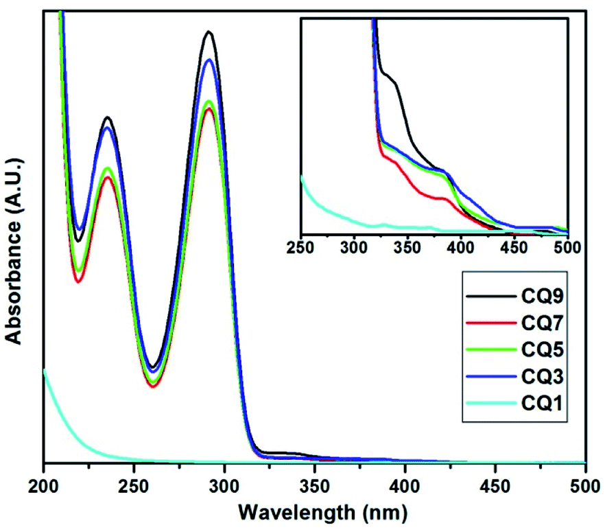Fig. 1 UV-vis absorption spectrum of C QD (inset) expanded spectrum.

Fig. 2 shows the QD photographed under long-range UV light (365 nm). Since all of the QD possessed the same transparency under daylight, only one of the samples is shown. Unarguably, the luminescence of the QD increases with an increase in nitrogen doping. As can be observed, CQ1 fails to show prominent luminescence. However, the change in colour from transparent (under daylight) to indigo is visible, and it gradually progresses to brighter light blue or aqua in the rest of the QD.

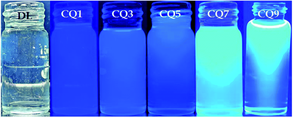Fig. 2 The images of the prepared C QD under daylight (DL) and long-range UV light (365 nm).

Fluorescence (FL) spectroscopy of the C QD was carried out with a PerkinElmer LS-55 instrument using an excitation wavelength of 290 nm, and the obtained result is shown in Fig. 3. CQ1, which showed minimal UV-vis absorption, gives two uneven emission peaks in FL spectroscopy. In the rest of the QD, a small initial emission peak below 400 nm appeared. In order to properly assess the emission peaks, Gaussian fitting for multiple peaks was applied using Origin 7.0 software. The obtained two distinct emission peaks of each QD are shown in Fig. 4, while the peak positions are tabulated in Table 1.

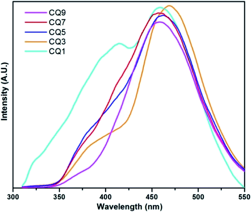Fig. 3 Fluorescence spectroscopy of the C QD.

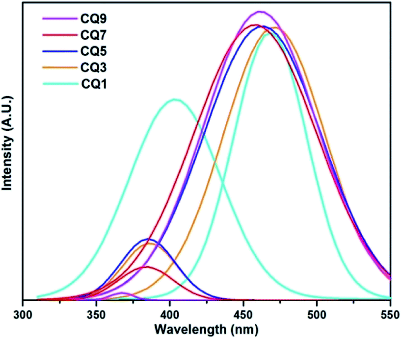Fig. 4 Gaussian fitting of the FL curves.

Table 1 FL peak positions of the C QD

	FL spectra		Gaussian fitted FL spectra
	Peak 1	Peak 2	Peak 1	Peak 2
CQ1	403.42	458.67	403.57 ± 3.93	468.26 ± 2.28
CQ3	386.58	468.42	386.35 ± 0.42	470.95 ± 0.12
CQ5	382.80	461.92	385.20 ± 0.55	462.94 ± 0.23
CQ7	374.70	458.67	383.77 ± 0.88	458.10 ± 0.24
CQ9	369.26	457.61	367.36 ± 0.36	461.66 ± 0.12

---

The reason for the strong emission of these QD could be attributed to the presence of surface states owing to the conjugated bonds. The presence of various functional groups leads to different surface state energy levels, which are responsible for the emission characteristics of the C QD.³² The emission peaks of CQ3 to CQ9 are quite uniform in nature, which is suggestive of consistency in the structure of the QD. The full width at half maximum (FWHM) of the peaks are rather wide, which suggests a wider distribution in the particle size of the QD. Overall, the emission peaks suggest the formation of high-quality C QD. As can be observed from Table 1, the emission peaks estimated from Fig. 3 are pretty close to the ones obtained from Gaussian fitting. The peak 1 position in the FL spectra, as well as the Gaussian fitted counterpart, are found to shift gradually towards the lower wavelength, which could be due to the decrease in size of the QD or increase in their surface states. At this stage, either of the conditions shall result in shifting of the emission peaks towards higher energy. However, with the exception of CQ1, the peak 2 of FL spectra also showed a gradual blue shift.

The functional group analysis of the QD was carried out using Agilent Cary 630 Fourier Transform Infrared (FTIR) spectroscopy technique within the range of 600–4000 cm⁻¹. For this a drop of the sample was made to come in contact with the probe. Since the QD are in aqueous state, the presence of the O–H stretch at ∼3350 cm⁻¹ was inevitable, as shown in Fig. 5. It also suggests the presence of the N–H stretch. The sharp peak at ∼1640 cm⁻¹ denotes the C=C stretch, N–H bend and C=N stretching. The structures of citric acid and uric acid are shown in Fig. 6.

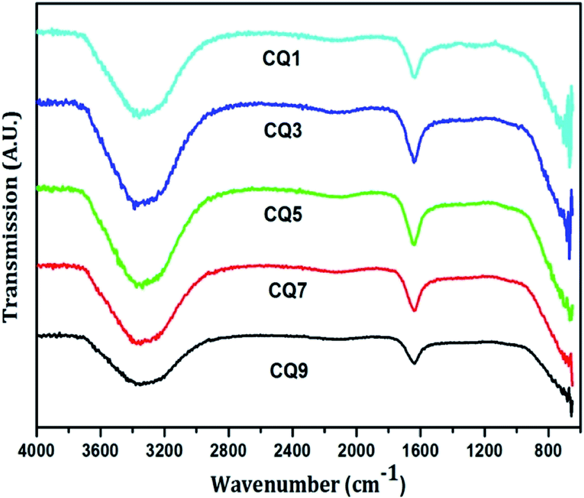Fig. 5 FTIR spectra of the QD.

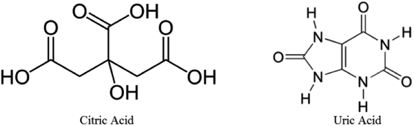Fig. 6 Structures of citric acid and uric acid.

There is no hint of the presence of any carboxylic acid or any ring type formation of the C QD. The characteristic peaks of citric acid appearing at ∼1720 cm⁻¹, corresponding to C=O, and at ∼1100 and 1210 cm⁻¹, corresponding to C–O, are not present in Fig. 5. Furthermore, the C–N stretch and bending peaks characteristic of uric acid found at ∼1028, 1124 and 1310 cm⁻¹ are also absent. Hence, this clearly eliminates the possibility of the precursors being present in their raw form, and confirms the presence of only nitrogen-doped C QD.

The Raman spectrum of the C QD was measured using micro-Raman model STR 500 with an excitation laser source of 532 nm. Since the FTIR analysis showed almost identical result for the different C QD, the Raman analysis was carried out for the highly fluorescent CQ9 only. The obtained result is shown in Fig. S4 (ESI).† It may also be noted that the intensity of the laser source was reduced to 0.1% for obtaining the result, owing to the extremely high fluorescence emission. Moreover, as reported previously, the used laser source has an impact on the band's positions of the carbon materials.³³ A broad D band is observed at 1369 cm⁻¹ with a shoulder 2D band appearing at ∼3014 cm⁻¹. Such broad bands originated from the presence of defects (surface states in the case of QD). As reported previously, when the number of defects in a material are large, it starts behaving like an amorphous one.³⁴ Fig. 5 indicates no presence of any ring type/graphitic peak. Hence, the G band might be completely absent. In such a scenario, the QD has only surface defects instead of any defined geometry, thereby leading to the occurrence of only defect bands in the Raman analysis.

Electrical study

The cyclic voltammetry (CV) study of the C QD was carried out to analyse its oxidation and reduction potential. A CV study was carried out using a CHI 604D electrochemical workstation in the voltage range of −2 V to +2 V at a scan rate of 0.05 V s⁻¹. A three-electrode setup was made with Pt wires as the working and counter electrode, and Ag/AgCl as the reference electrode, dipped in the aqueous C QD solution. A distance of 5 mm was kept between the two Pt wires.

The CV was carried out in three conditions – dark, 1 sun condition (light), and long-range UV (365 nm), with 9 sweep segments in each. The CV of CQ5 is shown in Fig. 7 with an expanded region in the inset. The CV of the rest of the QD is given in the ESI (Fig. S1–S3†), except CQ1 since it did not give any observable pattern.

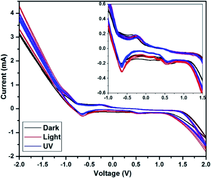Fig. 7 CV study of CQ5 (inset) expanded initial region.

Under dark condition, the segments are perfectly overlapping with one another, with no change in the maximum value of current at −2 V or +2 V. However, under UV and light condition, the QD show its photon responsive nature, owing to the maximum value of the current increasing after each segment. The obtained maximum value of the current is higher in the light condition compared to that under UV light, which affirms its responsiveness to visible light. The redox potential of the QD is almost overlapping in all three conditions, which confirms the absence of any permanent physiochemical change in CQ5 because of light exposure. The first oxidation peak is obtained at −0.65 V, followed by a miniature one at 0.56 V. The corresponding reduction peaks were obtained at −0.25 V and 0.44 V. It is expected that the obtained wide electrochemical window should serve well for its application in solar cells. The CVs of CQ3, CQ5, and CQ9 shown in Fig. S1, S2, and S3,† respectively, depict similar responses under the given conditions.

Electron microscopy

The HRTEM image of CQ5 was obtained using JEOL JEM-1011. For this purpose, a drop of the aqueous QD was placed on a carbon grid and the solvent was allowed to evaporate at room temperature. Fig. 8 shows the TEM image of the C dots, where most of the recognizable ones are marked in red circle. The calculated average size of the dots was 3.4 nm. The formed dots seem to be perfectly circular in shape, which is much clearer in the inset image of Fig. 8. Since there was not a major change in the absorption or emission characteristics of the different QD, a major variation in size was also not expected.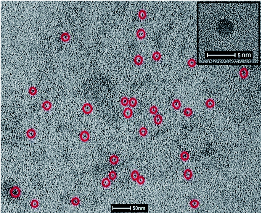

Fig. 8 TEM image of CQ5 (inset) enlarged view of CQ5.

J–V analysis

Since UV and FL studies showed no difference in the QD due to increased nitrogen doping, CQ5 was chosen randomly as the sensitizer. The solar cells were analysed for their current–voltage characteristics under a halogen lamp using a CHI 604D electrochemical workstation. The obtained characteristics of the two solar cells with an active area of 0.25 cm² under 1 sun condition is shown in Fig. 9, and the obtained values are presented in Table 2. A small increase in V_oc is observable in S2 compared to S1, signifying possible tuning of the band-alignment owing to the addition of C QD. A significant increase in the generation of charge carriers also occurred due to the absorption of a larger number of photons, which is justified well by the almost two-fold increase of J_sc. The resultant increase in efficiency is also ∼2.5 times.³⁵ In all cases, the current at 0 V was noted to be less than that at higher potential values. This makes the characteristics show lower FF and relatively high maximum current than its J_sc. Owing to the use of the polymer-based electrolyte, a polarization effect on the cell characteristics is bound to appear. The reason for the same has been explained in detail in one of our previous papers.³⁶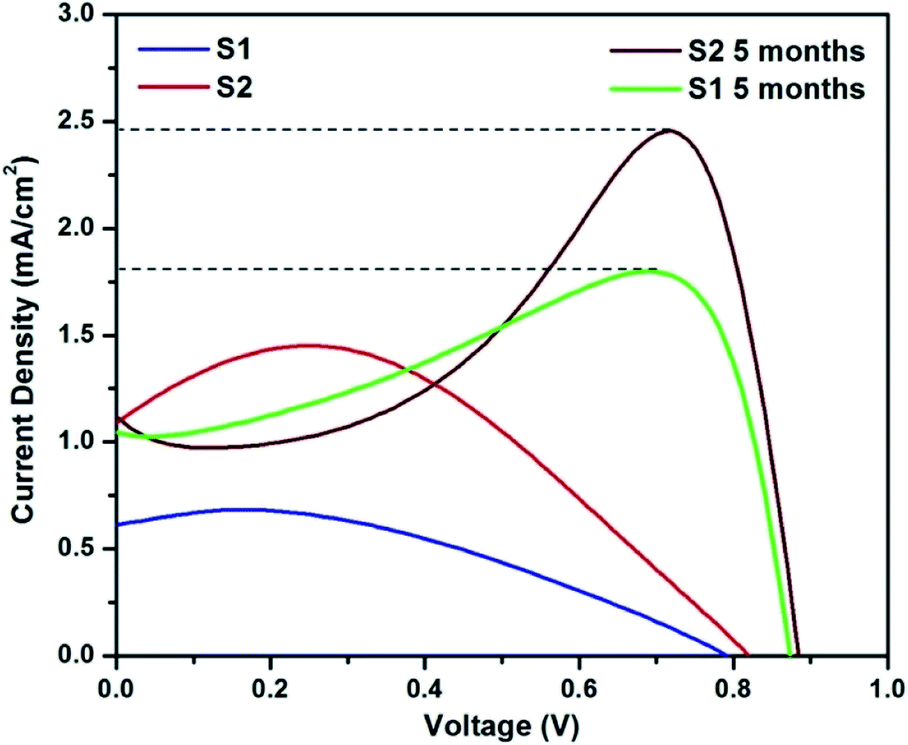

Fig. 9 J–V characteristics of the solar cells.

Table 2 The various obtained parameters of the solar cells

Solar cells	Voc (mV)	Jsc (mA cm^−2)	FF (%)	η (%)	Rs (Ω)	Rt (Ω)	Rc (Ω)	τ (ms)
S1	784	0.61	45.1	0.22	20.96	48.89	493.80	5.1
S2	820	1.10	59.8	0.54	33.19	62.16	513.60	8.2

---

To further check the stability of the cells, their J–V characteristics were analysed after an inactive period of 5 months, and the obtained characteristics are shown in Fig. 9. A significant improvement in the V_oc of the two cells can be seen, which would have most probably happened in the initial 72 h (electrode formation period in polymer-based cells).^24,37 Since the cell was used after a dormant period of 5 months, the formation of a strong polarization cloud over the electrolyte was unavoidable and the same is visible in the J–V pattern. The maxima in current were observed at much higher potential, and almost two times higher than the J_sc values. In fact, this maximum value of current should be extrapolated to the 0 V and noted as J_sc, which eventually shall give much higher FF and efficiency. However, to avoid any confusion, we have used the measured value of J_sc and only indicated the possible J_sc values by a dotted line in the figure. Nevertheless, the cell was active with almost similar efficiency even after a dormant period of 5 months.

Impedance analysis

The impedance analysis of the solar cells was carried out at 1 sun condition using a CHI 604D electrochemical workstation. The cells were subjected to an ac potential of 10 mV in the frequency range of 100k to 0.1 Hz at open circuit condition. The obtained Nyquist plots were followed by curve fitting and are shown in Fig. 10. The equivalent circuit used for analysis is given in the inset of Fig. 10.^24,30 The obtained values of R_s (series resistance), R_t (resistance between counter electrode and electrolyte) and R_c (resistance between working electrolyte and electrolyte) are given in Table 2. Owing to the additional layer of C QD, a small increase in impedance across the junctions of S2, compared to S1, can be observed. The comparatively high value of interfacial resistance is primarily attributed to the use of the polymer electrolyte, which does provide stability to the cells, but at the cost of a lower current. The value of R_s ranging between 20–30 Ω is pretty high, whereas an ideal value for a good-performance device should be a maximum of 10 Ω. This value is however consistent with our previous studies.^24,29 In addition, the use of a polymer electrolyte led to the R_t value between 50–60 Ω. Lowering of this value would help in improving the overall device performance. Furthermore, the value of R_c ranging in the order of 500 Ω is expected in such devices, but if this value could be decreased with some modification in polymer electrolyte, then the improvement shall be reflected in the J–V characteristics.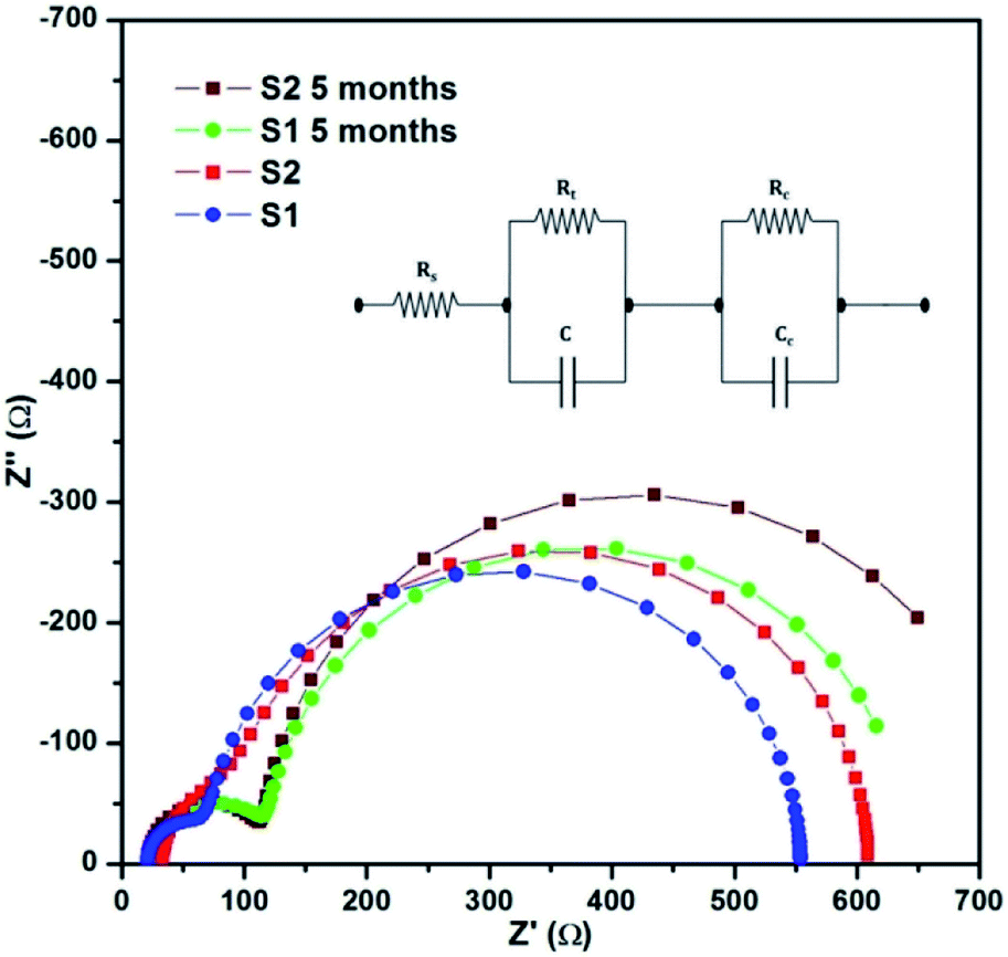

Fig. 10 Impedance analysis of the solar cells (inset) equivalent circuit.

The impedance analysis was also carried out after a period of five months, and an increase in both R_t and R_c can be observed. The long inactive period would have led to the shrinkage of the polymer chain in the device, thereby leading to the loss of flexibility, resulting in increased junction resistance. However, the impedance pattern stayed the same, which suggests no permanent physical or chemical alternation in the device.

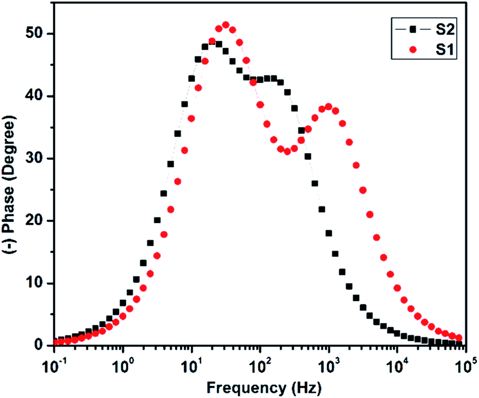
The Bode plot was derived from the impedance data, and is shown in Fig. 11. The electron lifetime could be estimated by the following formula (1).

τ_n = 1/2πf_max (1)

where ‘τ_n’ is the electron lifetime and ‘f_max’ is the peak frequency obtained in the low frequency region, which caters to the charge transfer process happening at the working electrode and electrolyte interface.

Fig. 11 Bode plot of the solar cells.

The calculated electron lifetime for the two solar cells S1 and S2 was 5.1 ms and 8.2 ms, respectively. The increased electron lifetime in S2 could be attributed to the decrease in recombination with an additional photon trapping layer of C QD, which not only helped in enhancing the band-alignment, but also accelerated the electron transfer process.

Time-dependent analysis

The time-dependent current and voltage analysis of the two cells was carried out in dark and 1 sun condition (light). The measurements were carried out using a CHI 604D electrochemical station. ‘Bulk electrolysis with coulometry’ mode was used for measuring the time-dependent current, while ‘open circuit potential-time’ was used for the time-dependent voltage measurement. For the time-dependent current analysis, a potential equal to the V_oc of the device was applied in order to protect it from any damage. The run time for each measurement was 300 s and the obtained results are shown in Fig. 12A to D.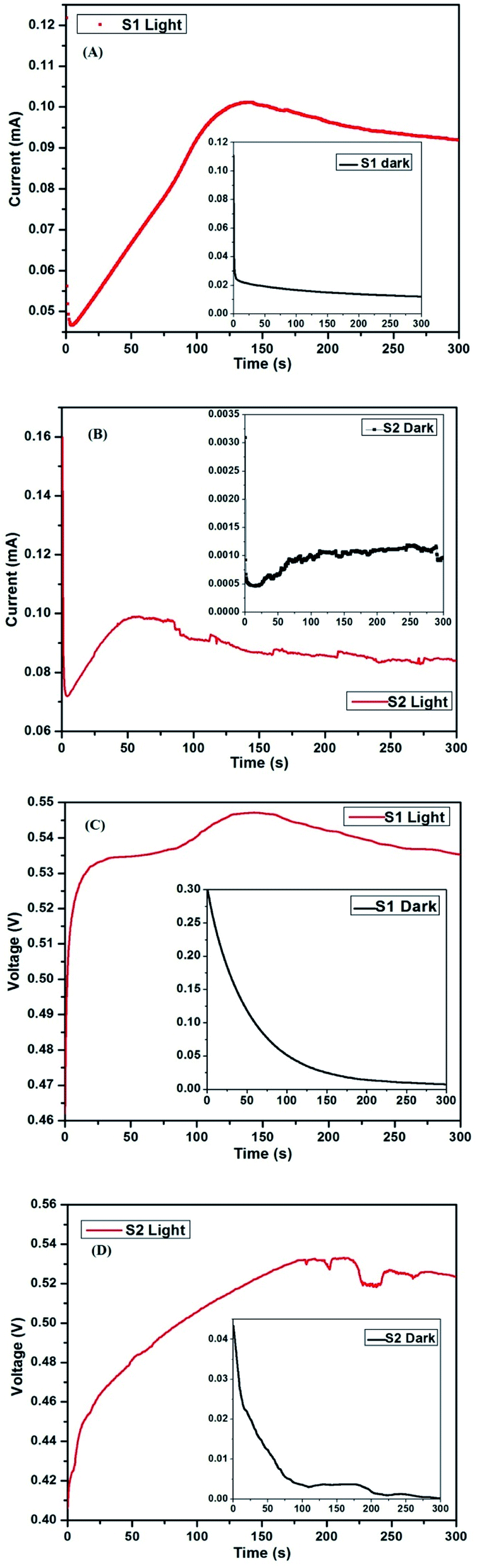

Fig. 12 (A and B) Current vs. time of S1 and S2 in light condition (inset – dark condition) (C and D) voltage vs. time of S1 and S2 in light condition ((inset – dark condition)).

As discussed previously, S2 has an additional layer of only C QD compared to S1. In the current vs. time analysis (Fig. 12A and B), both cells start showing a similar trend where the initial high current drops within a matter of seconds, followed by an increase. The time taken by S1 to achieve the peak current is ∼135 s, following which, it declines a little before the current saturates. On the other hand, the time taken by S2 to achieve peak current is ∼55 s, following which, it declines before saturating. The minor rise and fall in current value between time 75 s to 300 s may be due to the small fluctuations in the halogen lamp intensity. However, the same effect is not visible in S1, which suggests a higher level of radiation sensitivity of S2.

Furthermore, in the case of the dark condition of the two cells shown in the inset of Fig. 12A and B, both cells show a fast decrease in current initially, following which, S1 shows a gradual smooth decline. However, S2 shows a minor rise in current before progressing towards saturation. Owing to the presence of QD, the decrease in the value of the current with time is not as smooth compared to S1. This is due to the distinct ability of the QD to harness the infra-red (IR) radiation.^38,39

In the case of time-dependent voltage analysis, as shown in Fig. 12C and D, S1 shows an initial fast rise in voltage before gradually progressing towards a peak, following which, it drops down slowly to the peak voltage obtained during the initial few seconds. S2, on the other hand, shows a gradual increase in voltage with time. Beyond 175 s, the fluctuation is again present due to the slight change in halogen intensity, which if neglected, then we can see that the voltage is almost saturated. Similar to the current analysis, the voltage of S1 under dark condition shows a gradual decrease before saturating down to a few mV. On the other hand, the voltage does not show a smooth decrease in the case of S2 owing to the presence of QD. Another important thing to note is the starting voltage and current under dark condition in both cells. S2 is much more sensitive to radiation, and therefore starts at much lower voltage and current. The presence of voltage and current even in dark condition was conventionally not desired for solar cells. However, at present, cells with such properties are welcomed and explored for the possibility of use at lower light conditions.

The cell parameters (current and voltage) were monitored with time with the intention to understand if any permanent effect due to polarization had occurred during the exposure and/or measurements. The experimental setup for the measurement is shown in Fig. 13. An external circuit was prepared on a bread board using a carbon resistor of 2.4 kΩ, aluminium wires and two multi-meters. No other sophisticated instrument was employed for measurement.

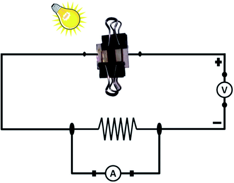Fig. 13 The schematic diagram employed for real-time solar cell measurement.

The current and voltage at different time intervals were measured using a multimeter under continuous irradiation with a halogen lamp at 1 sun condition with no external biasing. The peak temperature attained for the surrounding air was 56 °C. For avoiding any rise in temperature, a cooling fan was adjusted near the setup for blowing normal air around the setup. The obtained results for S1 and S2 are shown in Fig. 14A and B, respectively. After an almost instantaneous rise in the current and voltage, a small drop is noticed, followed by a rise, which ended to a stable value. This real-time activity of the solar cells is quite helpful in understanding their working.

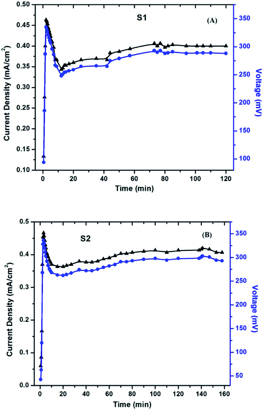Fig. 14 Current density and voltage measurement with rest to time under real-time conditions for (A) S1 and (B) S2.

The initial rise that appears as a sharp peak in the figures is due to the obvious photo-response of the cells upon illumination. The subsequent drop in current is attributed to the electrode formation, which is a well-known phenomenon, especially in polymer electrolyte-based devices, and has been observed in solar cells as well.⁴⁰ The gradual increase to a stable value is the actual time-dependent performance of the cells. This increase in current includes the effects of an increase in the ambient temperature upon continuous exposure of light, and also due to the stabilized folding–unfolding of the polymer chain. Once all of these activities get stabilized, the current attains a stable value. The voltage across the cells has also been noted and plotted against time (shown in the same Fig. 14 A and B). A similar explanation stands for the photo-voltage also. As can be seen from Fig. 14, around 60 min is required for the device to start giving stable output values. The values of the current and voltage are almost comparable in both S1 and S2.

Conclusions

The synthesis of N-doped aqueous C QD has been carried out successfully by hydrothermal method. Furthermore, the HRTEM image revealed an average particle size of 3.4 nm. The increase in nitrogen doping did not produce any significant change in the UV-vis absorption or FL emission, but a prominent change in luminescence of the QD was observed. The CV study showed that the QD were responsive to light, and had a wide electrochemical window. The C QD co-sensitized solar cell proved to possess better characteristics than the corresponding DSSC. The impedance analysis revealed high impedance at the junction, which is predominantly due to the use of the polymer electrolyte. The electron lifetime obtained from Bode plot confirmed the increase in electron lifetime in the cell employing C QD. Furthermore, the various time-dependent current voltage analyses revealed the real-time functioning of the solar cells. C QD proves to be a valuable candidate as a sensitizer in sensitized solar cells for future application. If the size of these C QD can be tuned, then they can be used efficiently in a graded structured quantum dot solar cell for providing better cell characteristics.

Author contributions

K. S. – conceptualization, data curation, formal analysis, investigation, methodology and writing original draft, R. M. M. – funding acquisition, resources, S. S. – resources, review and editing, B. B. – project administration, supervision, validation, visualization, review and editing.

Conflicts of interest

There are no conflicts to declare.

Acknowledgements

The author K. S. is thankful to CSIR, India for providing the Senior Research Fellowship (SRF, 09/1078(0002)/18 EMR-I) and to UGC, India for providing the UGC-DS Kothari Postdoc Fellowship (No. F. 4-2/2006 (BSR)/CH/20-21/0247). The authors are thankful to Prof. M. P. Deshpande, Department of Physics, Sardar Patel University for carrying out the Raman analysis. The financial assistance as Incentive to Senior Faculties under the Institute of Eminence Scheme (Dev. Scheme No. 6031) from Banaras Hindu University is gratefully acknowledged.

References

1. Z. Yang, T. Xu, Y. Ito, U. Welp and W. K. Kwok, J. Phys. Chem. C, 2009, 113, 20521.
2. U. O. Krašovec, M. Berginc, M. Hočevar and M. Topič, Sol. Energy Mater. Sol. Cells, 2009, 93, 379.
3. K. Kakiage, Y. Aoyama, T. Yano, T. Otsuka, T. Kyomen, M. Unno and M. Hanaya, Chem. Commun., 2014, 50, 6379.
4. K. Kakiage, Y. Aoyama, T. Yano, K. Oya, J. I. Fujisawa and M. Hanaya, Chem. Commun., 2015, 51, 15894.
5. E. M. Sanehira, A. R. Marshall, J. A. Christians, S. P. Harvey, P. N. Ciesielski, L. M. Wheeler, P. Schulz, L. Y. Lin, M. C. Beard and J. M. Luther, Sci. Adv., 2017, 3, eaao4204.
6. T. K. Das, P. Ilaiyaraja and C. Sudakar, ACS Appl. Energy Mater., 2018, 1, 765.
7. Y. Cui, H. Yao, J. Zhang, T. Zhang, Y. Wang, L. Hong, K. Xian, B. Xu, S. Zhang, J. Peng and Z. Wei, Nat. Commun., 2019, 10, 1.
8. W. Nie, H. Tsai, R. Asadpour, J. C. Blancon, A. J. Neukirch, G. Gupta, J. J. Crochet, M. Chhowalla, S. Tretiak, M. A. Alam and H. L. Wang, Science, 2015, 347, 522.
9. X. Zhang, X. Ren, B. Liu, R. Munir, X. Zhu, D. Yang, J. Li, Y. Liu, D. M. Smilgies, R. Li and Z. Yang, Energy Environ. Sci., 2017, 10, 2095.
10. K. S. Novoselov, A. K. Geim, S. V. Morozov, D. Jiang, Y. Zhang, S. V. Dubonos, I. V. Grigorieva and A. A. Firsov, Science, 2004, 306, 666.
11. X. Xu, R. Ray, Y. Gu, H. J. Ploehn, L. Gearheart, K. Raker and W. A. Scrivens, J. Am. Chem. Soc., 2004, 126, 12736.
12. P. G. Luo, S. Sahu, S. T. Yang, S. K. Sonkar, J. Wang, H. Wang, G. E. LeCroy, L. Cao and Y. P. Sun, J. Mater. Chem. B, 2013, 1, 2116.
13. B. De and N. Karak, RSC Adv., 2013, 3, 8286.
14. H. Li, X. He, Z. Kang, H. Huang, Y. Liu, J. Liu, S. Lian, C. H. A. Tsang, X. Yang and S. T. Lee, Angew. Chem., 2010, 122, 4532.
15. J. R. Macairan, D. B. Jaunky, A. Piekny and R. Naccache, Nanoscale Adv., 2019, 1, 105.
16. R. Singh, S. Kashayap, V. Singh, A. M. Kayastha, H. Mishra, P. S. Saxena, A. Srivastava and R. K. Singh, Biosens. Bioelectron., 2018, 101, 103.
17. X. Sun and Y. Lei, Trends Anal. Chem., 2017, 89, 163.
18. Y. Wang and A. Hu, J. Mater. Chem. C, 2014, 2, 6921.
19. J. B. Essner and G. A. Baker, Environ. Sci.: Nano, 2017, 4(6), 1216.
20. H. K. Sadhanala and K. K. Nanda, J. Phys. Chem. C, 2015, 119(23), 13138.
21. H. K. Sadhanala, J. Khatei and K. K. Nanda, RSC Adv., 2014, 4(22), 11481.
22. L. Liu, X. Yu, Z. Yi, F. Chi, H. Wang, Y. Yuan, D. Li, K. Xu and X. Zhang, Nanoscale, 2019, 11(32), 15083.
23. H. Lim, Y. Liu, H. Y. Kim and D. I. Son, Thin Solid Films, 2018, 660, 672.
24. K. Surana, S. Konwar, P. K. Singh and B. Bhattacharya, J. Alloys Compd., 2019, 788, 672.
25. S. Kakroo, K. Surana and B. Bhattacharya, J. Electron. Mater., 2020, 49(3), 2197.
26. P. K. Singh, R. K. Nagarale, S. P. Pandey, H. W. Rhee and B. Bhattacharya, Adv. Nat. Sci.: Nanosci. Nanotechnol., 2011, 2(2), 023002.
27. B. Bhattacharya, J. Y. Lee, J. Geng, H. T. Jung and J. K. Park, Langmuir, 2009, 25(5), 3276.
28. J. Cong, X. Yang, Y. Hao, L. Kloo and L. Sun, RSC Adv., 2012, 2(9), 3625.
29. K. Surana, M. G. Idris and B. Bhattacharya, Appl. Nanosci., 2020, 10, 3819.
30. K. Surana, R. M. Mehra and B. Bhattacharya, Opt. Mater., 2020, 107, 110092.
31. D. Carolan, C. Rocks, D. B. Padmanaban, P. Maguire, V. Svrcek and D. Mariotti, Sustainable Energy Fuels, 2017, 1(7), 1611.
32. F. Arcudi, L. Đorđević and M. Prato, Angew. Chem., 2016, 128(6), 2147.
33. R. P. Vidano, D. B. Fischbach, L. J. Willis and T. M. Loehr, Solid State Commun., 1981, 39(2), 341.
34. C. Pardanaud, G. Cartry, L. Lajaunie, R. Arenal and J. G. Buijnsters, C, 2019, 5(4), 79.
35. B. Mistry, H. K. Machhi, R. S. Vithalani, D. S. Patel, C. K. Modi, M. Prajapati, K. R. Surati, S. S. Soni, P. K. Jha and S. R. Kane, Sustainable Energy Fuels, 2019, 3(11), 3182.
36. K. Surana, N. A. Jadhav, P. K. Singh and B. Bhattacharya, Appl. Nanosci., 2018, 8, 2065.
37. K. Surana, I. T. Salisu, R. M. Mehra and B. Bhattacharya, Opt. Mater., 2018, 82, 135.
38. I. M. Dharmadasa, O. Elsherif and G. J. Tolan, J. Phys.: Conf. Ser., 2011, 286, 012041.
39. T. Morioka and Y. Okada, Phys. E, 2011, 44, 390.
40. B. Bhattacharya, H. M. Upadhyaya and S. Chandra, Solid State Commun., 1996, 98, 633.

---

Footnote

† Electronic supplementary information (ESI) available. See DOI: 10.1039/d1ra07634e

---