Optimization of metamaterials and metamaterial-microcavity based on deep neural networks

Abstract

Computational inverse-design and forward prediction approaches provide promising pathways for on-demand nanophotonics. Here, we use a deep-learning method to optimize the design of split-ring metamaterials and metamaterial-microcavities. Once the deep neural network is trained, it can predict the optical response of the split-ring metamaterial in a second which is much faster than conventional simulation methods. The pretrained neural network can also be used for the inverse design of split-ring metamaterials and metamaterial-microcavities. We use this method for the design of the metamaterial-microcavity with the absorptance peak at 1310 nm. Experimental results verified that the deep-learning method is a fast, robust, and accurate method for designing metamaterials with complex nanostructures.

---

1. Introduction

Metamaterials are novel artificial composite materials with unique properties not found in nature. With special properties, metamaterials have several applications in various fields. Photonic metamaterials play the role of an import in cloaking, antennas, subwavelength imaging, optical sensors, light modulation, optical polarization control, broadband perfect absorber, etc.^1–13 Metamaterials are often composed of a set of small, carefully engineered, regular structures such as spots, rings, rods, or a three-dimensional geometry. These are then fabricated as an array to obtain a metamaterial with certain desirable bulk behaviors.¹⁴ Two-dimensional metamaterials are also well known as metasurfaces. Several metamaterial structures such as split-ring resonators, negative refractive index fishnet, letter-shaped structures, and common geometric structures with symmetry and asymmetry^15–18 have been presented in the past two decades and most of them are important designs for different applications. Among them, the split-ring structure has been extensively used and will continue to be used because it can support narrow Fano resonance, trapped-mode magnetic resonances, and, quasi-bound states in the continuum (BIC).^19–29 Optical properties of single-layer metamaterials such as reflectance, transmittance and absorptance are generally a function of wavelength only when the structure and material of the metamaterial are fixed. If we want to provide functionalities on demand for flexible applications of metamaterials, temporal or space modulation of metamaterial-based devices is needed. Several methods such as adding a mirror to accommodate a Fabry–Pérot microcavity to modulate optical response by nanomechanics or using light to actuate individual metamaterial elements on demand with different mechanical resonances have been proposed.^30,31 The optimal design of such metamaterial structures remains challenging.

Several methods such as the finite difference time domain (FDTD) and finite element method (FEM) are applied for simulating the optical properties of split-rings with a certain structure; however, it is difficult and time consuming to optimize all the possible features of the split-ring structure. Therefore, the final design may not be the most appropriate one for the application. Many new methods such as artificial neural networks and deep neural networks (DNNs) have been proposed in recent studies to aid metamaterial design.^32–37 Here, we theoretically and experimentally demonstrated the usage of a DNN to achieve the forward prediction and inverse design of a split-ring aperture metamaterial. For the forward prediction of the spectral response of the metamaterial, we first generated original training data using COMSOL Multiphysics, and then trained the neural network (NN) using Keras in Python, and finally predicted the spectral response for arbitrary parameters of the split-ring. For the inverse design of the split-ring metamaterial, i.e., from the desired spectral response to the structural parameters, three different methods were discussed and compared in this study. The first method is training the NN inversely by setting the spectral response as the input data and setting the parameters of the split-ring as label data. The second method involves fixing the pretrained weights of the forward prediction and setting the parameters of the split-ring as trainable input data for training. The last method realizes a new network by connecting the inverse design NN and the pretrained forward prediction NN. The pretrained forward prediction NN and the tandem NN inverse design method were verified by experimental data, respectively. The results demonstrated that they are in excellent agreement. Notably, this method has a big priority for solving the one-to-many problem of the inverse design of metamaterials (one spectral response corresponding to several parameter combinations).

This paper is organized as follows: Section 2 introduces the forward prediction NN. Section 3 discusses the three methods for the inverse design of the split-ring metamaterial. Section 4 verifies the forward prediction NN and the inverse design method by experimental data. Section 5 proposes the optimization of metamaterial-microcavity. The conclusions are presented in Section 6, followed by the methods.

2. Forward prediction

Fig. 1 shows the forward prediction and the inverse design processes.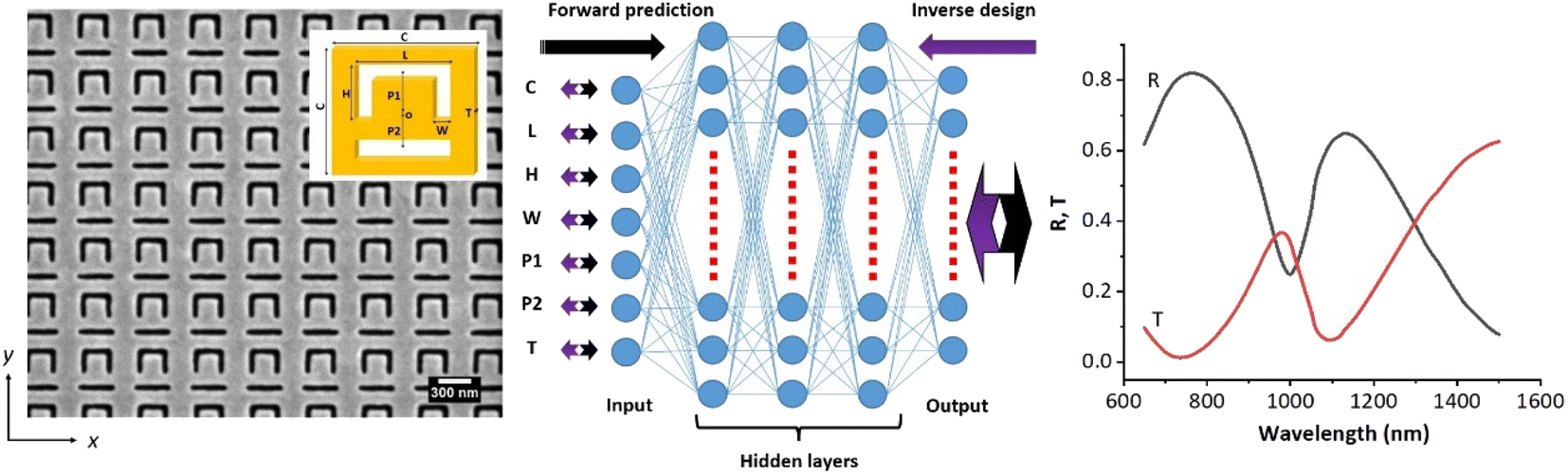

Fig. 1 Overview of the forward prediction and inverse design process by the DNN. Seven parameters (C, L, H, W, P1, P2 and T) of the split-ring are applied as training data. A DNN with four layers is adopted for the forward prediction and the inverse design. The input and output layers interchange for the forward prediction and inverse design. Three hidden layers have 100 neurons each. The spectral response for the reflectance (R) or transmittance (T) of the split-ring with arbitrary parameters can be rapidly predicted by the trained NN. Inset is the diagram of the split-ring cell.

Seven parameters of the split-ring including the cell size (C), slot length (L), slot height (H), slot width (W), upper and lower central positions of the slot (P1 and P2), and finally the thickness of the split-ring (T) can determine the entire structure of the split-ring metamaterial, and therefore are selected as the input data of the NN. There are four layers in the NN. The three hidden layers have 100 neurons each, and the output layer provides a one-dimensional vector with 86 elements covering the broadband spectral data (650–1500 nm with the step of 10 nm). Forward predictions of the reflectance (R) (or transmittance (T)) of the y-polarized light of the split-ring metamaterial can be obtained from the NN using the input parameters and pretrained weights. For inverse design, the spectral response of the y-polarized light is set as the input data. After training the NN, the predicted parameters of the split-ring are obtained accordingly. Through the pretrained weights, the exact parameters of the split-ring for the expected spectral response of the metamaterial can be obtained. Gold was used as the metal film of the split-ring metamaterial in this study, and the substrate of the metamaterial was silicon nitride. We set the range of each parameter as follows: C (300–500 nm), L (150–450 nm), H (130–230 nm), W (40–60 nm), P1 (100–180 nm), P2 (100–180 nm), and T (40–60 nm). For different C, we set different ranges of L, H, P1 and P2 to maintain the split-ring within the cell and without overlap. The above parameters were divided into five values separately, resulting in a total of 78 125 combinations. Furthermore, these parameter combinations were simulated using COMSOL Multiphysics. The simulation results including the reflectance and transmittance of each group of parameters were obtained simultaneously and used as the input data separately for the DNNs with Keras, 90% (10%) of which was training data (validation data). All input data were divided by 500 nm (maximum value of cell size) and normalized to values of 0–1. This can facilitate training and faster solution convergence. In forward prediction, a continuous value between 0 and 1 is predicted, which is a common type of machine-learning problem called regression. Therefore, the following model architecture was adopted. The fully connected network for this application included four layers and 100 neurons per hidden layer and a total of 29 686 parameters including the input and output layers need to be trained. The mean squared error ‘mse’ loss function, ‘adam’ optimizer, and mean absolute error ‘mae’ metric were used for compilation, and ‘sigmoid’ activation was added to all hidden layers; there was no activation in the last layer.

After training, we used the trained model to predict three types of split-ring structures with new parameters that are not present in the training or validation dataset. Fig. 2 compares different spectral responses of the NN prediction results and COMSOL simulation results with the same parameters. The purple, green, and red data represent the specified combination of test parameters, respectively (see Table S1 in the ESI). The prediction results are in good agreement with the simulation results, not only in the smooth ranges but also in the peaks and dips. This establishes that the trained NN can well predict any split-ring structure rapidly (sub-second), although the model is trained with each parameter only five times.

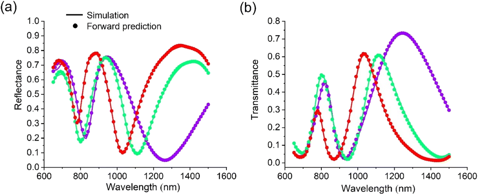Fig. 2 Comparison of the prediction and simulation results of the reflectance (a) and transmittance (b) for the three types of split-ring structures (the parameters of each split-ring are given in the ESI†). The dots represent the NN forward predictions, whereas the lines represent the COMSOL simulation results.

3. Inverse design

In practice, we aim to obtain a specific spectral response at a certain wavelength. For example, we expect a split-ring metamaterial with a transmittance peak at a wavelength of 1000 nm. This can be achieved using several deep learning approaches^{32,33,38–42} such as training the NN inversely, setting the input data as trainable weights by fixing the pretrained weights (optimization of input data), or building a new NN composed of a pretrained forward prediction NN and an inverse design NN, also called tandem NNs. We applied each of these three methods for inverse design in this study and chose the best one for further applications.

Inverse training of the NN (as shown in Fig. 1) implies that the forward prediction NN can be used inversely; hence, the input layer has 86 elements based on the spectral response of the split-ring (650–1500 nm with a step of 10 nm), and the output layer has seven elements (C–T) representing the predicted parameters of the split-ring. In addition, this network is similar to the forward prediction network. For optimization of input data, we applied the forward prediction NN, but fixed all the pretrained weights and only set the input data as trainable (as shown in Fig. S2(a)†). For training the tandem NNs, it consists of an inverse design NN and a forward prediction NN. All the pretrained weights from the forward prediction NN are fixed in the new network. The spectral response data are the input as well as output data for training the tandem NNs (as shown in Fig. S2(b)†). After training, the trained NN can be used to predict any spectral response or extract the transition layer weights as the parameters of the split-ring for COMSOL simulation. To verify the three inverse design methods, we used the reflectance and transmittance data (simulation results from COMSOL with C–T (nm) of 333, 272, 151, 52, 130, 132 and 55, respectively) as the input data to obtain the predicted parameters of the split-ring. After the parameters of the split-ring were predicted, we simulated the structure again in COMSOL, and compared the simulation spectrum (inverse predicted spectrum) with the previous input data (expected spectrum) to evaluate the accuracy. It is to be noted here that the predicted parameters of the split-ring are generally different from the initial parameters. Fig. 3(a) and (b) display the expected and the predicted reflectance and transmittance with the three different methods. To evaluate the accuracy of each method, we compared all the test data and used the ‘mse’ to determine the best solution for the inverse design of a split-ring aperture. The results show that training the tandem NNs is a little better than training the NN inversely, meanwhile optimization of input data is not suitable for this application. Therefore, we apply training the tandem NNs for inverse design in the subsequent sections.

Fig. 3 Three types of inverse design methods to predict the expected reflectance and transmittance of the split-ring metamaterial: (a) and (b) comparison of the inverse predicted reflectance and transmittance of the split-ring by the three different inverse design methods with the expected reflectance and transmittance. The predicted data are obtained from corresponding NNs. The expected data are determined through COMSOL simulation.

4. Experimental verification of the split-ring metamaterial

In this section, we used the split-ring metamaterial samples to verify the above methods experimentally. Metamaterial samples were fabricated through the thermal evaporation of gold on a silicon nitride substrate, followed by focused ion beam milling of the gold film. The reflectance and transmittance of each metamaterial sample were determined using a microspectrophotometer (CRAIC Technologies) with a halogen light source.

The first sample with parameters shown in Fig. 4(a) was fabricated for testing the forward prediction. The experimental reflectance (black-line) of the first metamaterial sample and forward predicted reflectance using the pretrained forward prediction NN (red-line) are depicted in Fig. 4(a). Inset is the scanning electron micrograph (SEM) image of the metamaterial. Parameters C–T of the split-ring aperture measured through SEM (shown in the figure) are the input data of the pretrained NN. The experimental and predicted transmittance of this sample are depicted in Fig. 4(b). Furthermore, the experimental and predicted reflectance (transmittance) of the second metamaterial sample is displayed in Fig. S4(a) and (b) in the ESI.

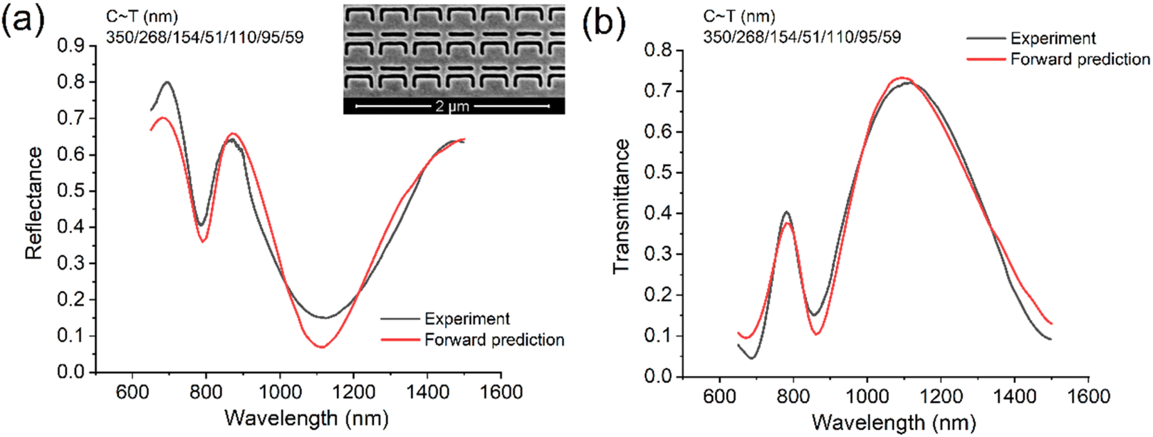Fig. 4 Comparison of the experimental and forward predicted values by the pretrained NNs. (a) Experimental reflectance and forward predicted reflectance of the metamaterial with a cell-size of 350 nm (the measured parameters of the split-ring metamaterial are shown in the figure). (b) Experimental transmittance and forward predicted transmittance of the metamaterial. Inset is the SEM image of the metamaterial sample.

The other samples were fabricated to test the inverse prediction of the split-ring metamaterial. The experimental reflectance data of the metamaterial sample were added to the pretrained tandem NNs, and inverse prediction of the input spectral data was directly obtained from the output data of the tandem NNs (similar to Fig. 3(a)). The experimental reflectance (transmittance) as well as the inverse predicted reflectance (transmittance) of the sample is shown in Fig. 5(a) and (b). In this case, the exact parameters of the split-ring can be ignored, which are only used for the transition layer in Fig. S2(b).† Furthermore, the experimental reflectance (transmittance) and inverse predicted reflectance (transmittance) of another sample are depicted in Fig. S5(a) and (b).†

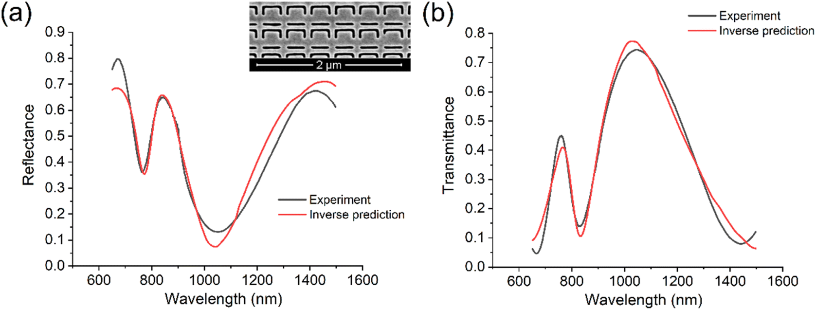Fig. 5 Inverse prediction of the experimental spectral data by the pretrained tandem NNs. Experimental reflectance (a) and transmittance (b) of the metamaterial sample compared with corresponding inverse predicted reflectance and transmittance. Inset is the SEM image of the metamaterial sample.

The forward prediction results in Fig. 4 almost match the corresponding experimental data around three peaks; hence, the predicted results are satisfactory considering the measurement error of the split-ring size as well as the fact that the corner of the slot is not a perfect right angle. Therefore, it can be concluded that forward prediction based on an NN has the same accuracy as the theoretical simulation and can be applied as a practical method for designing split-ring metamaterials. Concerning the inverse prediction of the experimental data in Fig. 5, all the predicted results well match the experimental data indicating that the tandem NNs can learn the exact details of the metamaterial and “accommodate” certain flaws of the metamaterial, not just fitting the training data. The transition layer in Fig. S2(b) in the ESI† contains the predicted parameters of the split-ring, which can be retrieved for further usage. It may not be possible to simulate and optimize such inverse prediction directly with COMSOL because a spectrum corresponds to a couple of parameter combinations (one-to-many problem).

5. Optimization of metamaterial-microcavity

The optical reflectance, transmittance, and absorptance of a single-layer metamaterial are important parameters in practice. However, single-layer metamaterials (<100 nm) can hardly achieve extreme reflectance (transmittance or absorptance) due to the limited interaction between light and the metamaterials. Theoretical analysis and experimental results show that the metamaterial-microcavity composed of a single-layer metamaterial and an optical mirror can greatly improve the optical response characteristics.^29,30 In this case, its overall optical reflectance will be determined by the reflection and transmission coefficients of the single-layer metamaterial as well as the gap of the microcavity, and can be described theoretically as follows:²⁹where r and t are the complex Fresnel reflection and transmission coefficients of the single-layer metamaterial, m is the reflection coefficient of the mirror, α = 2πd/λ is the phase change and d is the distance of the gap. The external force can modulate this distance, thus changing the optical response of the microcavity. In particular, magnetic field sensors which use Lorentz force to change the distance of the gap are an important application field of this kind of metamaterial-microcavity.³⁰ Next, we expect this sensor to be able to transmit signals over long distances by optical fiber for non-contact and harsh environmental applications. Therefore, the 1310 nm infrared light in the telecommunication band is a good choice for optical fiber communication, and we also hope the sensor has high sensitivity and a wide dynamic range around this band. This requires that the overall reflectance of microcavity R in eqn (1) reaches the minimum value at the wavelength of 1310 nm with certain d.

Hence, the reflection coefficient r of the single-layer metamaterial is an important parameter to consider in the following design. We first needed to design the single-layer metamaterial with the minimum reflectivity at the wavelength of 1310 nm. This can be easily done by the above inverse design method (more details in the ESI†). After the inverse predicted parameters of the single-layer metamaterial (C–T (nm), 498/296/217/56/173/149/49) were obtained, we then plotted the overall reflectance of metamaterial-microcavity according to eqn (1), as shown in Fig. 6. The overall reflectance minimum (maximum) at the wavelength of 1310 nm covers the range of the gap from 1450 nm to 1620 nm (1140 nm to 1270 nm), and this can tolerate the gap error during the sample fabrication step. Fig. 7(a) shows the SEM image of the metamaterial membrane and details of the metamaterial pattern with predicted parameters. We then tested the overall reflectance of the microcavity based on this metamaterial and compared it with the expected reflectance, as shown in Fig. 7(b). They are in good agreement around dips and peaks. As expected, we get a minimum reflectance at a wavelength of 1310 nm with a distance of a gap of 1580 nm. In fact, the real gap of metamaterial-microcavity may be a little different from 1580 nm used in sample fabrication because of gravity, but the results in Fig. 7(b) indicate that the gap is indeed in the range of 1450 nm to 1620 nm.

Fig. 6 Dependence of metamaterial-microcavity reflectance on gap and wavelength according to the inverse design parameters of the metamaterial. Inset is the 2D illustration of the metamaterial-microcavity.

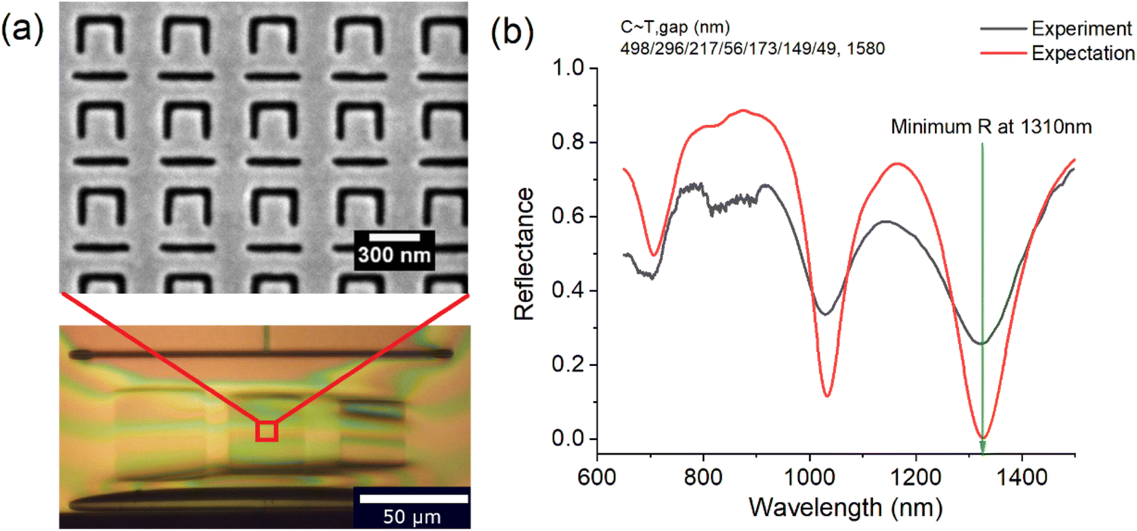Fig. 7 Metamaterial-microcavity and its optical reflectance. (a) SEM image of the fabricated metamaterial (top) and the whole membrane on the mirror (bottom). (b) Experimental and expected optical reflectance of metamaterial-microcavity. Inverse design parameters of the split-ring metamaterial and the distance of the gap are given in the inset.

6. Conclusions

We have demonstrated that DNNs are an efficient and fast tool for the optimization of split-ring metamaterials and metamaterial-microcavity. The pretrained DNNs verified with experimental data can automatically design metamaterials on demand forward and inversely. The optimized metamaterial pattern provided great convenience for the optimal design of metamaterial-microcavity and made it possible for other special applications. The proposed deep-learning-assisted metamaterial design method is a simple, fast, robust, and accurate method for studying split-ring metamaterials and metamaterial-microcavity, which is expected to play an important role in metamaterial design and applications.

7. Methods

7.1. Simulation

We used COMSOL Multiphysics 5.4 to generate the training, validation, and test data. A 3D wave-optics model with electromagnetic waves in the frequency domain was used in the simulation. The refractive index of gold was the interpolation of the Lorentz–Drude oscillator model. The geometry of the split-ring is shown in Fig. 1. A computer with dual Intel Xeon E5-2696 CPUs and 128 GB RAM required approximately five days to prepare all the data. We used the open source Keras⁴³ in Python to build the NN. The forward training NN included four layers; each of the three hidden layers had 100 neurons, and the output layer had 86 neurons covering a wavelength range of 650–1500 nm with a step of 10 nm. We used ‘sigmoid’ as the activation function in the hidden layers and there was no activation function in the output layer. The optimizer, loss, and metric applied for the forward prediction were ‘adam’, ‘mse’ and ‘mae’, respectively. Approximately 4 min was required to completely train a type of spectral response such as the reflectance. For the inverse design, the required time for inverse prediction was similar to that for the forward prediction.

7.2. Metamaterial fabrication and characterization

The metamaterials were fabricated by the thermal evaporation of gold on a silicon nitride membranes, followed by focused-ion-beam milling of the gold film. The bottom mirror of microcavity is gold film. The reflectance and transmittance of each metamaterial sample were determined using a microspectrophotometer (CRAIC Technologies) with a halogen light source.

Data availability

The data that support the findings of this study are openly available in University of Southampton ePrints research repository at https://doi.org/10.5258/SOTON/D2428.

Author contributions

G. L. and J. Y. O. conceived the idea and designed the experiments. G. L. designed the samples and performed the theoretical simulations. J. Y. O. and Y. W. fabricated the samples. J. Y. O. and Y. W. performed the inspections of the samples and the optical measurements. J. Y. O. and G. L. performed the data analysis. G. L., Y. W. and J. Y. O. discussed and prepared the manuscript, and all authors reviewed it. J. Y. O. supervised the research.

Conflicts of interest

The authors declare no conflicts.

Acknowledgements

We acknowledge Dr Eric Plum from the University of Southampton for the beneficial discussion. This work is supported by the UK Engineering and Physical Science Research Council (grants EP/M009122/1 and EP/T02643X/1) and the Basic Scientific Research of Heilongjiang University (2020-KYYWF-0997), China.

References

1. D. Schurig, J. J. Mock, B. J. Justice, S. A. Cummer, J. B. Pendry, A. F. Starr and D. R. Smith, Science, 2006, 314, 977–980.
2. N. F. Yu and F. Capasso, Nat. Mater., 2014, 13, 139–150.
3. C. L. Holloway, E. F. Kuester, J. A. Gordon, J. O'Hara, J. Booth and D. R. Smith, IEEE Trans. Antennas Propag., 2012, 54, 10–35.
4. N. Liu, T. Weiss, M. Mesch, L. Langguth, U. Eigenthaler, M. Hirscher, C. Sonnichsen and H. Giessen, Nano Lett., 2010, 10, 1103–1107.
5. C. M. Soukoulis and M. Wegener, Nat. Photonics, 2011, 5, 523–530.
6. Z. Jacob, L. V. Alekseyev and E. Narimanov, Opt. Express, 2006, 14, 8247–8256.
7. T. Xu, Y. K. Wu, X. G. Luo and L. J. Guo, Nat. Commun., 2010, 1, 59.
8. C. H. Wu, A. B. Khanikaev, R. Adato, N. Arju, A. A. Yanik, H. Altug and G. Shvets, Nat. Mater., 2012, 11, 69–75.
9. A. V. Kabashin, P. Evans, S. Pastkovsky, W. Hendren, G. A. Wurtz, R. Atkinson, R. Pollard, V. A. Podolskiy and A. V. Zayats, Nat. Mater., 2009, 8, 867–871.
10. Q. Wang, E. T. F. Rogers, B. Gholipour, C. M. Wang, G. H. Yuan, J. H. Teng and N. I. Zheludev, Nat. Photonics, 2016, 10, 60–U75.
11. N. Liu, L. Langguth, T. Weiss, J. Kastel, M. Fleischhauer, T. Pfau and H. Giessen, Nat. Mater., 2009, 8, 758–762.
12. H. T. Chen, W. J. Padilla, J. M. O. Zide, A. C. Gossard, A. J. Taylor and R. D. Averitt, Nature, 2006, 444, 597–600.
13. Y. J. Huang, L. Liu, M. B. Pu, X. Li, X. L. Ma and X. G. Luo, Nanoscale, 2018, 10, 8298–8303.
14. J. Valentine, S. Zhang, T. Zentgraf, E. Ulin-Avila, D. A. Genov, G. Bartal and X. Zhang, Nature, 2008, 455, 376–379.
15. M. Kadic, G. W. Milton, M. van Hecke and M. Wegener, Nat. Rev. Phys., 2019, 1, 198–210.
16. C. M. Watts, X. L. Liu and W. J. Padilla, Adv. Mater., 2012, 24, OP98–OP120.
17. N. I. Landy, S. Sajuyigbe, J. J. Mock, D. R. Smith and W. J. Padilla, Phys. Rev. Lett., 2008, 100, 207402.
18. J. Y. Ou, E. Plum, L. Jiang and N. I. Zheludev, Nano Lett., 2011, 11, 2142–2144.
19. R. A. Shelby, D. R. Smith and S. Schultz, Science, 2001, 292, 77–79.
20. A. I. Kuznetsov, A. E. Miroshnichenko, Y. H. Fu, J. Zhang and B. Luk’yanchuk, Sci. Rep., 2012, 2, 492.
21. W. Withayachumnankul and D. Abbott, IEEE Photonics J., 2009, 1, 99–118.
22. T. Koschny, P. Markos, D. R. Smith and C. M. Soukoulis, Phys. Rev. E, 2003, 68, 065602(R).
23. M. Chen, Z. Xiao, Z. Cui and Q. Xu, Opt. Commun., 2021, 502, 127423.
24. H. M. Silalahi, Y. P. Chen, Y. H. Shih, Y. S. Chen, X. Y. Lin, J. H. Liu and C. Y. Huang, Photonics Res., 2021, 9, 9.
25. A. V. Novitsky, V. M. Galynsky and S. V. Zhukovsky, Phys. Rev. B, 2012, 86, 75138.
26. D. R. Chowdhury, R. Singh, J. F. O’Hara, H. T. Chen, A. J. Taylor and A. K. Azad, Appl. Phys. Lett., 2011, 99, 2075.
27. I. V. Shadrivov, D. A. Powell, S. K. Morrison and Y. S. Kivshar, Appl. Phys. Lett., 2007, 90, 201919.
28. Z. Qiao, X. Pan, F. Zhang and J. Xu, IEEE Photonics J., 2021, 1.
29. P. Cencillo-Abad, N. I. Zheludev and E. Plum, Sci. Rep., 2016, 6, 37109.
30. G. Lan, J.-Y. Ou, D. Papas, N. I. Zheludev and E. Plum, APL Photonics, 2022, 7, 036101.
31. J.-Y. Ou, E. Plum and N. I. Zheludev, Appl. Phys. Lett., 2018, 113, 081104.
32. M. H. Tahersima, K. Kojima, T. Koike-Akino, D. Jha, B. Wang, C. Lin and K. Parsons, Sci. Rep., 2019, 9, 1368.
33. J. Peurifoy, Y. Shen, L. Jing, Y. Yang, F. Cano-Renteria, B. G. DeLacy, J. D. Joannopoulos, M. Tegmark and M. Soljacic, Sci. Adv., 2018, 4, eaar4206.
34. S. Inampudi and H. Mosallaei, Appl. Phys. Lett., 2018, 112, 5.
35. J. Q. Jiang and J. A. Fan, Nano Lett., 2019, 19, 5366–5372.
36. X. G. Luo, Adv. Mater., 2019, 31, 21.
37. Z. A. Kudyshev, A. V. Kildishev, V. M. Shalaev and A. Boltasseva, Nanophotonics, 2021, 10, 371–383.
38. S. So, J. Mun and J. Rho, ACS Appl. Mater. Interfaces, 2019, 11, 24264–24268.
39. D. Liu, Y. Tan, E. Khoram and Z. Yu, ACS Photonics, 2018, 5, 1365–1369.
40. L. Shelling Neto, J. Dickmann and S. Kroker, Opt. Express, 2022, 30, 986–994.
41. Q. Wu, X. Li, W. Wang, Q. Dong, Y. Xiao, X. Cao, L. Wang and L. Gao, ACS Omega, 2021, 6, 23076–23082.
42. Y. Chen, J. Zhu, Y. Xie, N. Feng and Q. H. Liu, Nanoscale, 2019, 11, 9749–9755.
43. Resources can get from https://keras.io and https://github.com/keras-team/keras.

---

Footnote

† Electronic supplementary information (ESI) available. See DOI: https://doi.org/10.1039/d2na00592a

---