
 Open Access Article
 This Open Access Article is licensed under a
 Creative Commons Attribution 3.0 Unported Licence
Ab initio study of lithium intercalation into a graphite nanoparticle†
Julian
Holland
 ae,
Arihant
Bhandari
ae,
Denis
Kramer
bce,
Victor
Milman
d,
Felix
Hanke
d and
Chris-Kriton
Skylaris
*ae
ae,
Arihant
Bhandari
ae,
Denis
Kramer
bce,
Victor
Milman
d,
Felix
Hanke
d and
Chris-Kriton
Skylaris
*ae
aSchool of Chemistry, University of Southampton, Southampton, SO17 1BJ, UK. E-mail: C.Skylaris@soton.ac.uk
bFaculty of Mechanical Engineering, Helmut-Schmidt University, Hamburg, 22043, Germany
cEngineering Sciences, University of Southampton, Southampton, SO17 1BJ, UK
dBIOVIA, Unit 334 Cambridge Science Park, Milton Road, Cambridge, Cambridgeshire CB4 0WN, UK
eThe Faraday Institution, Quad One, Becquerel Avenue, Harwell Campus, Didcot, OX11 0RA, UK
First published on 27th September 2022
Abstract
The process of Li intercalation is fundamental to the operation of Li-ion batteries and the computational modelling of this process, as atomic resolution would be of great benefit to the rational design of improved battery materials. Towards this goal, we present an approach and workflow for the simulation of Li intercalation which uses electrostatic considerations. These considerations use the electrostatic potential found from Density Functional Theory (DFT) calculations as a guiding principle to find favourable sites for Li intercalation. We test the method on graphite-based models of anodic carbon, graphite nanoparticles. The study of nanoparticles using first-principles methods is made possible thanks to linear-scaling DFT which allows calculations on larger numbers of atoms than conventional DFT. We show how our approach can reproduce the well-known Li staging and we investigate the electronic structure of the nanoparticle obtained via atomic charges and density of states analysis. We also compute the open circuit voltages of the structures via a convex hull formalism and find reasonable agreement with experiment with respect to the degree of Li intercalation. Our approach provides a novel route to simulating the intercalation process and, combined with linear-scaling DFT, can be used to investigate intercalation in complex nanoscale electrode structures.
1 Introduction
Li-ion batteries are charged and discharged by the intercalation and deintercalation of Li within electrodes through an electrolyte.1 The most popular anode material is graphite due to its high Li storage capacity, electrochemical stability, cycling stability, and affordability.2–8 For this reason Li intercalation into graphite has been the subject of intense study both experimentally9–14 and computationally.15–21 Other graphite-like anode materials such as graphenelyne,22 biphenylene monolayers,23 or even doped graphite24 have also been subject to intense study.Despite this, the mechanisms surrounding the charging and discharging of the graphite anode are still not fully understood.25–27 Recent experimental and computational investigations have focused on the entropic contributions of different stage formations,17,19,21 the transition between Li stages,11 and the kinetics of Li intercalation.17,18,20 Experimental results often differ from computational ones. For example, the voltage step profiles presented by Persson et al.18 were unable to match the experimental results presented by Stevens and Dahn28 even when including van der Waals (vdW) corrections.
A potential cause of the apparent mismatch between experiment and computation is that, until now, ab initio calculations have been primarily performed on bulk graphite. Graphite, in batteries, often occurs at the micro- or nano-scales.29,30 The incidence of particles occurring at the nano-scale is likely to increase with cell age due to the prevalence of cracking as the volume expands and contracts upon charging and discharging.31,32 It is possible that to reconcile computational and experimental results, the unique structural properties of the nanoparticle must be accounted for. This has proven difficult to model at electron resolution due to the large number of electrons present in a nanoparticle. Conventional density functional theory (DFT) scales at ![[scr O, script letter O]](https://www.rsc.org/images/entities/char_e52e.gif) (n3), where n is the number of atoms in the system, due to the need to perform computationally expensive processes such as diagonalization under the constraint of orthonormality. This puts an effective limit on the size of the system that can be studied using conventional DFT. Large-scale DFT calculations are possible due to the recent developments of linear-scaling DFT, where the computational cost scales at (n). We use ONETEP33 (cf. Section 2.1) because of the highly parallelizable nature of this program.
(n3), where n is the number of atoms in the system, due to the need to perform computationally expensive processes such as diagonalization under the constraint of orthonormality. This puts an effective limit on the size of the system that can be studied using conventional DFT. Large-scale DFT calculations are possible due to the recent developments of linear-scaling DFT, where the computational cost scales at (n). We use ONETEP33 (cf. Section 2.1) because of the highly parallelizable nature of this program.
Previously, we investigated graphite systems with intercalated34 and nucleated Li.35,36 These studies were performed on graphite slabs and we found energetic preferences for Li intercalation and nucleation at graphite edges. As experimentally used systems contain multiple edges, these types of effects can be studied in greater detail with a graphite nanoparticle. In this work, we advance understanding by focusing on Li intercalation into the graphite nanoparticle by adopting a novel Li placement strategy. This study can be further advanced to consider events of nucleation and dendrite formation on graphite nanoparticles by extending Li placement on surfaces as well (cf. Section 2.5).
Established methods such as cluster expansion37,38 have been used to simulate Li intercalation in bulk systems previously.18,39 However, these methods require the energy calculations of multiple extra configurations to find the lowest energy structures.37 This is computationally expensive, particularly when performing these calculations on large systems. Ran et al.38 partially address this issue by employing a group-subgroup transformation formalism to rigorously find structures for their bulk graphite system and eliminate a large portion of configurational space. This reduction of configurational space allowed them to identify a new extremely low ground state structure occurring at Li0.0625C6.
However, even with the impressive breakthroughs of Ran et al., an insurmountable disadvantage of this method is that it requires long-range, translational symmetry (i.e. the construction of a supercell).40 Methods such as cluster expansion or group sub-group transformation are unsuitable for dealing with large systems of low long-range symmetries, such as nanoparticles. Recently, Shen et al.41 demonstrated a method that used the charge density minimum for intercalating lithium ions and demonstrated it on a large number of common, bulk cathode materials. To insert Li they find the relaxed, unlithiated structures of the bulk cathode crystals and the respective local minima of charge density equating them to lithiation sites. The authors validated the use of charge density by calculating the binding energy of known Wyckoff sites in the crystals and compared them to their predictions. They found that the charge density predictions aligned with the Li atoms' site preference. They were also able to capture structural phenomena such as accurately reproducing which Li insertions would give topotactic insertions.
Given that the primary source of interaction in graphite intercalated compounds (GICs) between Li and C is electrostatic, we, instead, place Li atoms at the global minimum of the electrostatic potential within our system. After each lithiation, this method should only find structures that are close to the ground-state and therefore reduce the number of calculations needed to be performed (cf. Section 2.4). To validate our model we will be looking for a number of structural and electronic phenomena that we would expect to occur in graphite. The phenomena we validate against are detailed below.
• Li staging: Li intercalation occurs with a staging process whereby lithiation between graphite layers does not result in a uniform distribution. Li will preferentially populate sites between graphite layers that have already experienced some degree of lithiation, thus forming a layer of Li. The Li layers that form have a long-range symmetry that is dependent on the degree of global lithiation. The type of staging is dictated by the number of graphite layers between Li layers. If there is only one (i.e. full or close to full lithiation) then this is a stage I compound, if there are two it is a stage II compound, and so on.42
• AB to AA graphite shift: graphite's lowest energy state has its individual graphite sheets staggered. i.e. the centre of a graphite hexagon will have a carbon atom aligned directly above and below it. This is known as an AB structure. With increasing Li saturation the vdW forces between graphite sheets are weakened. They are replaced with Li–C interactions. As the lowest energy state for Li is directly above and below a centre of the graphite hexagon there is increasing preference, with increasing lithiation, for the graphite layers to slide over one another to accommodate the Li's optimum position.19,43 Therefore, a transition to an AA structure occurs where all C atoms in graphite layers are stacked directly on top of each other.
• Charge transfer: upon entering the graphite structure Li atoms give up their 2s electron to the C 2p orbitals. This plays an important role in the expansion of the graphite intercalated compound (GIC), as well as the staging process.11 Charge transfer can be probed through the analysis of local charges on atoms, as well as the electronic density of states (DOS).44
• Voltage step profile: direct comparison to experimental open circuit voltage (OCV) measurements can be made by plotting the calculated voltages from the ground-state structures against the degree of lithiation.18 To find the ground-state structures we draw a lower convex hull from all GICs we produce. These structures tend to be topotactic as we intercalate further until the threshold for the next structure is met.41
Comparison to experiment and prior computational studies through the aforementioned metrics will enable us to assess the quality of our model. We will also be able to highlight the differences that occur when moving to the nanoscale with our nanoparticle.
The paper is structured so that in Section 2.1 we briefly outline the linear-scaling DFT code that we use, ONETEP. In Section 2.2, we benchmark exchange–correlation functionals that account for long-range forces for a graphite-like system and select the best functionals to move forward with. We then define our nanoparticle and calculation properties in Section 2.3. The intercalation methodology is outlined in Sections 2.4 and 2.5. We outline the results in Section 3, splitting them into structure (Section 3.1), local charge (Section 3.2), electronic density of states (Section 3.3), and voltage step profiles (Section 3.4). Finally, we perform further calculations to investigate the cause of the lack of AB to AA shift as we intercalate our nanoparticle in Section 3.5.
2 Methodology
2.1 ONETEP
All calculations were performed with ONETEP, a linear-scaling DFT code, where the computational cost scales linearly with the number of atoms as opposed to cubic scaling in conventional DFT.33,45 ONETEP is based on reformulating DFT in terms of the one-particle density matrix. This matrix is expressed in terms of atom-centred, non-orthogonal generalised Wannier functions (NGWFs).46 The NGWFs are in turn expanded with a basis set of periodic sinc (psinc) functions which are related to plane waves through a unitary transformation.47 This allows us to truncate the one-particle density matrix and thus achieve linear scaling for large enough systems.2.2 Modelling graphite properties
When modelling graphite computationally using DFT, a careful approach to functional selection must be made. Intraplanar bonding can be reproduced easily enough with most functional choices, due to the well-defined nature of covalent bonds. However, the interplanar interactions are determined by weaker, long-range effects. These interactions are not accounted for with generalised gradient approximation (GGA) functionals48–51 and spuriously accounted for with local density approximation (LDA)52 functionals. For this reason, many non-local functionals53–57 and empirical correction terms58–62 were developed.This work aims to add Li atoms between the graphite layers at the most favourable sites. This adds a further layer of complication as the electrostatic interactions of Li–C are stronger than the C–C vdW interactions.18 An accurate representation of vdW interactions is therefore essential for realistic Li intercalation.
Starting from pure graphite we consider a number of functionals to determine which one best models the interlayer binding energy and interlayer spacing. Our results were compared to other computational and experimental studies. We consider the following non-local functionals: rVV10,53 AVV10s,54 vdW-DF,55 vdW-DF2,56 optPBE,57 optB88.57 We also consider PBE with the Grimme D2 empirical correction term.58
The calculations were performed on a 640 atom graphite structure with periodic boundary conditions.33 The structure is 10 layers high, with each layer consisting of 64 C atoms (cf.Fig. 1a). To find the interlayer spacing we follow the technique outlined by Bramley et al. to expand our unit cell.63 We iterate upon this technique by only varying a single lattice parameter, or interlayer spacing (c), as demonstrated by Siersch et al.,64 between 2.978 and 4.964 Å. The kinetic energy cutoff was kept constant throughout (732.32 eV) while the number of psinc functions, that form our basis set, along the z-axis were increased.65
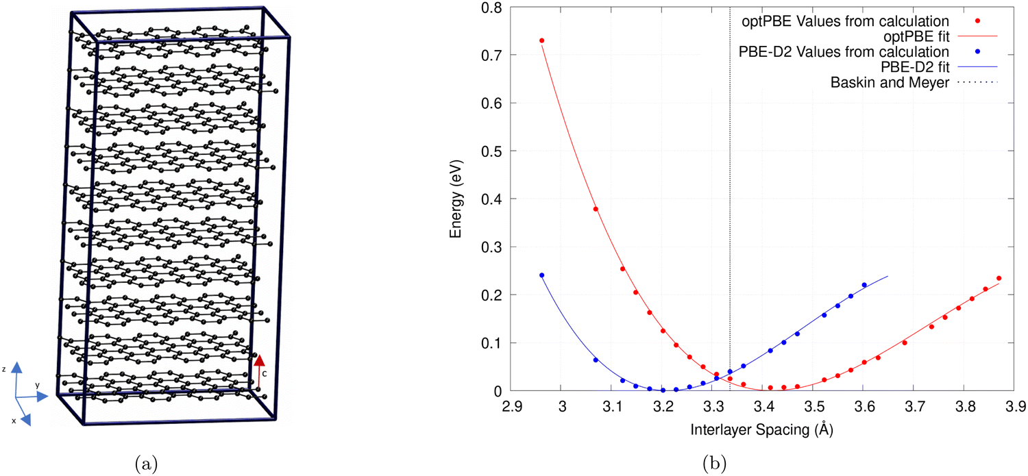 | ||
| Fig. 1 (a) Periodic graphite structure used to test various non-local functionals and empirical correction terms. (b) The relationship between the interlayer spacing of bulk graphite and the total energy. A third-order Birch–Murnaghan equation of state was used to fit this plot. Results of the optPBE non-local functional and PBE with the D2 correction term are shown.63,65 Experimental results by Baskin and Meyer are also shown.68 | ||
Plotting the total energies against the volume of the simulation cell allows us to fit a third-order Birch–Murnaghan equation shown in Fig. 1b.64,66,67 As only the interlayer spacing is varied this is what is displayed on the x-axis instead of volume. We use the least mean square method to fit this equation to our results. The minimum of this plot gives the lowest energy simulation cell volume and therefore the ideal interlayer spacing (c).
The interlayer binding energy, Eint, was found by considering the energy difference between the bulk, Ebulk, with the minimum energy interlayer spacing for each functional used, and that of infinitely separated graphene sheets, Esep. In practice, we set our graphite system to have an interlayer spacing of 10.1 Å which should be far enough away that any long-range interactions are negligible.
 | (1) |
| Interlayer spacing (Å) | ||||
|---|---|---|---|---|
| Experiment | 3.3360 ± 0.000568 | |||
| Functional | Our results (ONETEP) | Chen et al.15 (VASP) | Hazrati et al.16 (VASP) | Lenchuk et al.72 (VASP) |
| LDA | — | 3.33 | — | — |
| LDA-D258 | — | 2.99 | — | — |
| PBE73 | — | 4.42 | 4.40 | 3.99 |
| PBE-D258,73 | 3.22 | 3.23 | — | — |
| PBE-D360,73 | — | — | — | 3.34 |
| rVV1053 | 3.36 | — | — | — |
| AVV10s54 | 3.48 | — | — | — |
| vdW-DF55 | 3.56 | — | 3.59 | 3.54 |
| vdW-DF256 | 3.51 | 3.51 | 3.51 | — |
| optPBE57 | 3.44 | 3.45 | 3.44 | — |
| optB8857 | 3.36 | 3.36 | 3.36 | 3.32 |
| optB86b57 | — | — | 3.31 | 3.29 |
| Layer binding energy (meV per atom) | ||||
|---|---|---|---|---|
| Experiment | 52 ± 5 Zacharia et al.69 | |||
| 31 ± 2 Liu et al.70 | ||||
| 35 ± 15 Benedict et al.71 | ||||
| Functional | Our results (ONETEP) | Chen et al.15 (VASP) | Hazrati et al.16 (VASP) | Lenchuk et al.72 (VASP) |
| LDA | — | 23.7 | — | — |
| LDA-D258 | — | 114.9 | — | — |
| PBE73 | — | 0.9 | 1.0 | — |
| PBE-D258,73 | 54.5 | 55.2 | — | — |
| PBE-D360,73 | — | — | — | 53 |
| rVV1053 | 70.4 | — | — | — |
| AVV10s54 | 65.3 | — | — | — |
| vdW-DF55 | 54.0 | — | 52.7 | 53 |
| vdW-DF256 | 53.4 | 52.1 | 52.0 | — |
| optPBE57 | 64.0 | 63.7 | 63.7 | — |
| optB8857 | 70.7 | 69.6 | 69.5 | 70 |
| optB86b57 | — | — | 69.9 | 70 |
In this table, we compare our binding energy and interlayer spacing values to experimental data and to other published DFT results. We do this to validate our findings and to establish the functional that predicts the most realistic graphite properties. Attention should be drawn to the disparate experimental layer binding energy values cited in Table 1. There is no definitive way to find the interlayer binding energy of graphite experimentally in the literature. There have, however, been several attempts to find a good approximation that we include in our table.69–71
As shown in Table 1, our calculated values for both interlayer spacing and interlayer binding energy are similar to and, in the case of interlayer spacing, often replicate the results found by Hazrati et al.16 and Chen et al.15 This demonstrates that the accuracy of ONETEP is comparable to that of plane-wave codes such as VASP.74 We find that rVV10 and optB88 functionals give the best overall interlayer spacing and PBE-D2, vdW-DF, and vdW-DF2 give interlayer binding energies similar to that reported by Zacharia et al.69
Chen et al.15 found PBE with the Grimme D2 dispersion correction to perform the best. They also find the C33 elastic modulus for comparison between functionals. Hazrati et al.16 chose the optB88 functional to move forward in their calculations. They selected it because it gave the best overall structure, which is reflected in our results, and this was deemed to be the most important feature for the type of calculations they were doing. However, they also note that optPBE performs equally well due to its better prediction of binding energy. Lenchuk et al.72 found vdW-DF to best recreate the structural and thermodynamic properties of graphite and Li intercalated graphite. It was the only functional to correctly estimate the shape of the voltage step profile without the need for correction.
With no apparent best functional we ran calculations using the Grimme D2 functional correction term58 championed by Chen et al.15 as well as the optPBE non-local functional57 as it gave close to experimental values for both metrics. This will allow a comparison of both the most common approaches to modelling vdW interactions, non-local functionals and empirical correction terms, for our system.
2.3 Nanoparticle
Our nanoparticle consists of 484 C atoms and is terminated with 108 H atoms. It is 4-layers thick with each layer consisting of 121 carbons and 27 hydrogens (Fig. 2). This structure was constructed using Materials Studio.75 Dangling carbon sigma bonds are terminated with H atoms because it is a naturally occurring structure, described by Andersson et al.30 This size of structure is considerably smaller than even the smallest nanoparticles used in anodes which typically consist of 1000s of atoms.30 This size was chosen as it has been shown that polycyclic aromatic hydrocarbon (PAH) dimers reach an assymtopic limit of interaction energy with increasing monomer C atom count.76 Circumcoronene (C54H18) was shown by Totton et al.76 to be approaching that limit. A similar limit was observed with the binding energy PAH adsorbing on to graphene with respect to number of aromatic rings by James and Swathi.77 We use this limit as a guide for our individual layer size. By more than doubling the C atom count in each sheet, compared to that of Circumcoronene, we are confident that our system is close enough to the limit to exhibit graphite-like binding energies. To ensure the completion of our calculations in a reasonable time frame, a necessity to validate the methods we wish to look at in this paper, we abstain from increasing the size of our nanoparticle further. The structure has enough layers to exhibit most of the natural properties of Li intercalation, such as staging and stacking which need several layers of C atoms to occur. Although, we do expect differences compared to bulk staging as evidence points to a minimum of 8 layers required to fully describe this process.78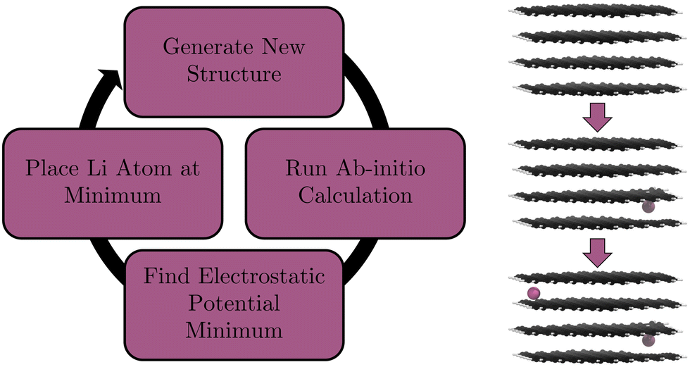 | ||
| Fig. 2 The workflow employed (left) to intercalate a graphite nanoparticle (right) with Li atoms using the electrostatic potential as a guide for Li placement. Li atoms are in pink, C atoms in black, and H atoms in white. | ||
Graphite-like structures such as this can be intercalated up to the LiC6 limit. A 484 C atom nanoparticle should therefore have around 80 Li sites. However, this is not a bulk structure and adsorption occurs both above and below the nanoparticle. Therefore an extra layer of sites needs to be accounted for. This would increase the number of lithiation sites to approximately 100. However, for the reasons that will be explained in Section 2.5, only the 60 internal Li intercalations are modelled. It should also be noted, given the geometry of our nanoparticle, if we were to assume all Li is perfectly spaced, as we discuss in Section 3.5, then the maximum Li intercalation limit is 42.
All nanoparticle calculations were performed using the generalised gradient approximation (GGA) exchange–correlation functional, PBE73 with the Grimme D258 dispersion correction or using the non-local optPBE functional57 (cf. Section 2.2). We use a kinetic energy cut-off value of 830 eV and a NGWF radii of 9.0 a0. The core electrons are represented using projected augmented waves (PAW)79 from the well-established80 GBRV pseudopotential library.81 For Li, all electrons were treated as valence because we expect Li electrons to move from the Li to the graphite structure. We do not want to artificially restrict this charge transfer by treating the 1s2 electrons as core electrons. Calculations were performed with ensemble-DFT (EDFT),82 spin polarisation, and utilised the quasi-Newton Broyder-Fletcher–Goldfarb–Shanno (BFGS) algorithm due to its stability and efficiency.83 Our geometry optimisation calculations use a displacement convergence tolerance of 1.5 × 10⁻²a0, an energy convergence tolerance of 1.5 × 10⁻⁶Eh, and a force convergence tolerance of 3 × 10⁻³Eha0−1. Periodic boundary conditions have been used. A sufficiently large, cubic simulation cell with a volume of 2.362 × 10⁵a03 was used to reduce interactions between the nanoparticle and its periodic images.33,84 This provides a vacuum between particles of over 53 a0 inline with the nanoparticle planes and 74 a0 orthogonal to the nanoparticle planes. We include an image of our nanoparticle in its simulation cell in our ESI,† to demonstrate the relative proportions of vacuum to system. All input files are provided in the ESI.†
2.4 Intercalation procedure
To place highly polarizable Li atoms in a structure, the optimal sites of intercalation need to be found. Chevrier and Dahn did this for amorphous Si anodes by identifying the largest open spaces available to the ion.85 Shen et al. did this via the use of charge density (cf. Section 1).41 We use the electrostatic potential minimum. The main interaction between an intercalated Li atom and the graphite is electrostatically driven. Therefore, using the electrostatic potential as a guide for finding favourable intercalation sites is a reasonable assumption to make. Here, we describe the practical procedure of the calculations undertaken. First, our initial unintercalated structure is relaxed with a DFT geometry optimisation. The electrostatic potential of this relaxed structure is output as a voxel cube file in ONETEP. We find the minimum value voxel in the simulation cell and translate the voxel's position to real space Cartesian coordinates. We then place a Li atom at this position. The script that processes the voxel cube file is provided in our ESI.† Then, we relax the structure with the newly-added Li atom, find the position where the electrostatic potential of this new structure is minimum, and place the next Li atom at the position of this minimum. We then run a single point calculation, find the position where the electrostatic potential is at its minimum, and place the third Li atom at this minimum. We repeat this process alternating between single point calculations and full geometry optimisation calculations until our structure is fully lithiated. Single point calculations are considerably lower in computational cost and given that our structure is relaxed regularly we do not expect a significant change in Li placement. We also perform a full geometry optimisation on our final structure. The workflow of this process is demonstrated in Fig. 2.2.5 Placement restriction
Initial nanoparticle calculations with the PBE-D2 functional had no restrictions on where the Li atoms could be placed. We observed pseudo-stage II Li atom distribution up to the 21st lithiation (Fig. 3b) if we ignore the basal plane adsorption. After this, populating of the central layer occurred and the structure became stage I. As we continued to lithiate, Li-metal accumulation on the basal planes was observed (Fig. 3c).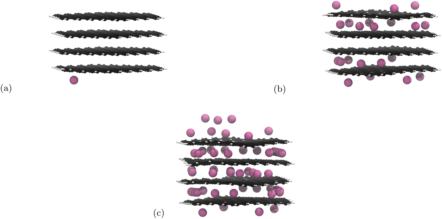 | ||
| Fig. 3 Li intercalation of graphite nanoparticle with unrestricted placement of Li. Li atoms are in pink, C atoms in black, and H atoms in white. Images of all structures can be found in our ESI.† (a) First Li atom is placed on the basal place of the structure. (b) 21 Li atoms intercalated in the graphite nanoparticle. Stage II stacking persists. (c) 51 Li atoms intercalated into the graphite nanoparticle. Stage II stacking is lost and there is a build up of lithium metal on the surface of the nanoparticle. | ||
The results yielded from the unrestricted placement of Li warrant further investigation, particularly with reference to Li–metal formation being more favourable than intercalation. Li-plating on anodes is an active area of research35,86 and is a topic that should be pursued in another project. Li on individual layers are not expected to interact significantly with Li on other layers.18 For this reason we restricted Li placement between the highest and lowest carbon atoms along the z-axis as any atoms adsorbed on the basal plane are unlikely to affect the internal structure. Because adsorption has been prevented, 60 Li atoms is now the theoretical maximum intercalation.
In our optPBE functional calculations, the structure of the graphite sheets became so flared that the Li were still able to adsorb to the basal plane as they could technically still be placed on the basal plane but below/above the highest/lowest C atom. To prevent this we added a 1 Å lithiation restriction zone around the highest and lowest C atoms.
3 Results and discussion
Using the procedure described in Sections 2.4 and 2.5 we intercalate our nanoparticle with Li atoms consecutively. This process is performed twice with different exchange–correlation functionals: PBE, with the D2 correction term, and optPBE (cf. Section 2.2).3.1 Structure
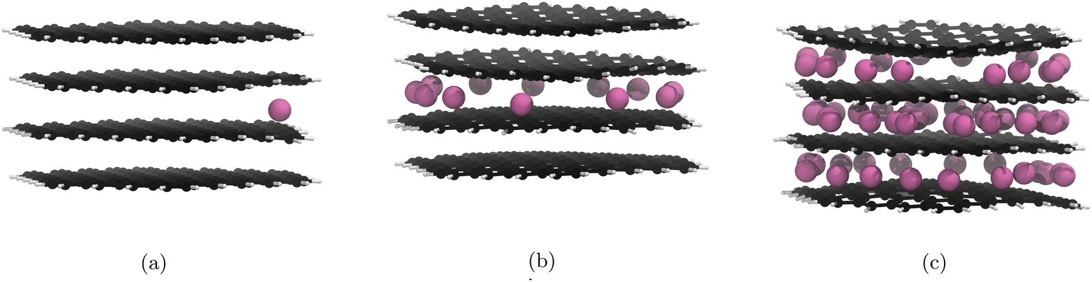
For the PBE-D2 functional we observe the formation of a stage II structure up to the 29th lithiation (Fig. 4b). This is approximately half of the theoretical lithiation maximum for intercalation of internal layers. If our system had aligned with the staging mechanism observed in bulk graphite,19 all sites in the upper and lower layers would be occupied before the filling of the central layer, i.e. a stage II structure up to the 40th lithiation. Further lithiations past the half-lithiated (30 Li) structure result in an early collapse to a stage I structure as the central layer is populated. The formation of a stage II structure is a promising result and demonstrates that the nanoparticle follows similar behaviour to what was observed by computational studies on bulk graphite.18,19 | ||
| Fig. 4 Significant geometry optimised GIC structures from Li intercalation with Li placement restrictions (cf. 3.5), using PBE with the D2 correction term. Li atoms are in pink, C atoms in black, and H atoms in white. Images of all structures can be found in our ESI.† (a) 1st lithiation, Li atoms fill the central layer after this point. (b) 29th lithiation, Li atoms start filling the central layer after this point. (c) 60th lithiation is the theoretical maximum lithiation. | ||
A similar pattern is observed for our optPBE calculations, whereby the initial intercalation layer choice makes future intercalations into that layer more likely (Fig. 5a). However, because our initial Li intercalation occurs in the central layer, with half as many possible sites available for stage II population, the breakdown to stage I occurs earlier (Fig. 5b).
 | ||
| Fig. 5 Significant geometry optimised GIC structures from Li intercalation with Li placement restrictions (cf. 3.5), using the optPBE correction functional. Li atoms are in pink, C atoms in black, and H atoms in white. Images of all structures can be found in our ESI.† (a) 1st lithiation, Li atoms fill the upper and lower layers after this point. (b) 12th lithiation, Li atoms start filling the upper and lower layers after this point. (c) 60th lithiation is the theoretical maximum lithiation. | ||
In both the optPBE and PBE-D2 calculations the early breakdown of stage II to stage I is observed. This breakdown is unlike the dilute phase transitions that are observed by Dahn25 and is instead due to the intercalation model preferring Li placement around the edges of the nanoparticle. We discuss the cause of this edge site preference in later Sections (cf. 4.2 and 4.5). The preference appears to be strong enough to forgo population in the centre of an already populated layer for an edge site on a different layer.
Both generated final structures (Fig. 4c and 5c) have an uneven distribution of Li atoms in individual layers. In the PBE-D2 structure, the upper layer has 17 Li atoms, the middle has 21 atoms, and the lower has 22. For optPBE, the disparity is more pronounced with the upper layer having 15 Li atoms, the central layer having 27 Li atoms, and the lower layer having 18 Li atoms.
This uneven distribution can be partially attributed to the preference of Li to populate the edges of the nanoparticle. This is because the edge-site preference is strong enough to overcome intra-layer Li–Li repulsion interactions thereby increasing the maximum capacity of individual layers in the nanoparticle. In the final structure, for our PBE-D2 calculations (Fig. 4c), some Li atoms were found to be within 2.7 Å of each other, as opposed to the 4.3 Å typically observed in bulk GICs. The same is true for our optPBE calculations. These structures are not fully saturated as there are numerous lithiation sites unfilled in the centre of the upper and lower layers. This is surprising, as if this were realised in experiments it could provide a route to exceeding the 372 mA h g−1 theoretical limit of energy storage for graphite without the stacking of layers of solid Li, as was observed by Küuhne et al.87
A theoretical study on how the particle size distribution of graphite affects the cell performance is presented by Röder et al.29 In this paper, they find that distributions with smaller graphite nanoparticles are less likely to degrade and have higher internal capacities compared to distributions with larger particles. Our observations of closer than typical Li placement in our nanoparticle could partially explain the increased capacity observed by Röder et al.29
While lithiation occurs primarily around the edge sites, at later intercalations, both functionals begin to favour the filling of the centre of the central layer over available edge sites on the upper and lower layers. This phenomenon appears earlier in the optPBE calculations than in the PBE-D2 calculations. This led to the final structure of our optPBE calculations (Fig. 5c) having a significantly more heavily populated central layer than its PBE-D2 counterpart (Fig. 4c). This demonstrates the drastic effect that different interpretations of the long-range forces have on the electrostatic potential of GICs. The earlier population of the centre of the nanoparticle in our optPBE calculations indicates either that the electrostatic potential is lowered in the centre of the central layer or the edge site electrostatic potential is raised at the upper and lower layer edge sites relative to our PBE-D2 calculations. We find the latter of these conclusions to be more likely for the reasons given below.
In our PBE-D2 calculations, we observe a 19.7% increase in interlayer spacing at the edges of the nanoparticle, where the majority of the lithiation occurs, and a 7.5% increase at the centre of the nanoparticle, where less lithiation occurs. For our optPBE calculations, we observe a 17.4% increase at the edge and a 2.88% decrease in the centre. It is likely that the geometry of our structures, decided in part by the interpretation of the long-range forces, is the direct cause for the different preferences of edge and centre sites between both functionals. The decreased space afforded to the edge sites in the optPBE calculations relative to the PBE-D2 calculations likely meant the electrostatic potential was slightly higher and the global minimum was now located within the relatively unaffected centre of the central layer. Experimental results observe a uniform 10.4% increase in interlayer spacing when comparing graphite (3.35 Å) to its fully lithiated GIC (3.70 Å).88 We would expect a larger increase in interlayer spacing in our nanoparticle compared to bulk calculations due to our structure being intercalated in a vacuum. This is because the nanoparticle lacks the pressure along the z-axis which is present in bulk graphite and serves to compact the structure. While this explains the larger than bulk graphite increases at the edges, it does not explain optPBE's decreasing centre, particularly when considering that the centre of the optPBE nanoparticle is more filled than its PBE-D2 equivalent. One possible description of this effect is that due to the lower uniformity of Li distribution and the lack of external pressure on the outer graphite layers increased deformation was allowed to occur. This increased “flaring” of the outer graphite layers can only be attributed to optPBE's interpretation of long-range forces. For PBE-D2 The C–C bond length increases by 0.012 ± 0.007 Å as we intercalated to 60 Li. For optPBE the bond length increased by 0.015 ± 0.007 Å. This bond length increase occurs primarily around the edges where the H termination occurs causing shorter C–C bonds due to the slight electronegativity difference (cf. Section 3.2). We do not anticipate this small an increase in bond length and therefore surface area to have a significant effect on properties such as Li capacity.
Given the uniqueness of our structure and how little literature there is surrounding the intercalation of graphite nanoparticles, it is hard to say which method out of optPBE and PBE-D2 generates the most realistic structure. For this reason, we will continue with the analysis of both.
We observe no shift from an AB to an AA structure, something we would expect to see if this were a bulk structure. We explore the cause behind this in Section 3.5.
3.2 Mulliken population analysis
To obtain some insight into the distribution of charges, we use Mulliken population analysis89 to partition the total charge density into point charges associated with individual atoms as intercalation occurs. For both functionals, in the unlithiated structures, this technique reveals that the edge C atoms, those directly bonded to H atoms, have a slight negative charge due to the difference in electronegativity (Fig. 6a and c). This leads to Li placement at sites closer to the more negatively charged C atoms. The placement of Li atoms at edge sites, which donate their electrons to the graphite structure (cf. Section 3.3), exacerbates the effect leading to more negatively charged edges in the lithiated structures (Fig. 6b). Another possible cause for the edge accumulation of Li atoms is the topological spin polarisation of the graphite edges as was observed by Peng et al.34 The authors note the prevalence of this effect is most extreme for zig-zag edges that are H-terminated. However, upon analysing the spin density of our nanoparticle at various stages of lithiation we saw no evidence of spin polarised states emerging as the ground-state. For both our calculations it is apparent that places where Li has intercalated result in a greater population of electrons in the surrounding carbons (cf.Fig. 6b and d). This replicates what has been observed in the literature for bulk graphite.90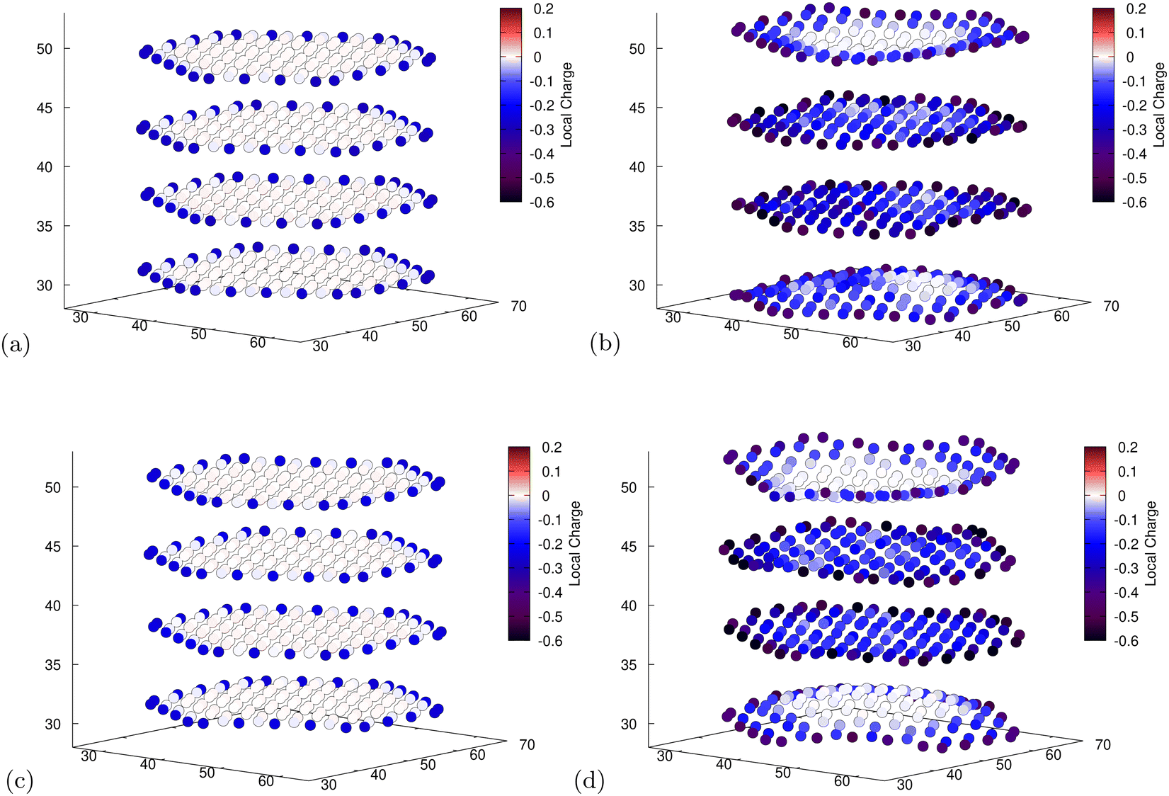 | ||
| Fig. 6 Mulliken population analysis for C atoms for the fully unlithiated (a and c) and fully lithiated (b and d) graphite nanoparticles. The axes are the spatial coordinates within the simulation cell in Bohr and the colour indicates the charge of individual C atoms. More detailed images for all individual atoms can be found in ESI.† (a) PBE-D2, 0 Li, electron population of C atoms. (b) PBE-D2, 60 Li, electron population of C atoms. (c) optPBE, 0 Li, electron population of C atoms. (d) optPBE, 60 Li, electron population of C atoms. | ||
3.3 Density of states
Further evidence for the transfer of electrons from the Li to the graphite nanoparticle can be found by examining the density of states (DOS). Comparing the total DOS (TDOS) of the nanoparticle to that of its fully lithiated counterpart and shifting both graphs so their Fermi levels occur at 0 reveals a shift in the TDOS to the left as lithiation occurs (cf.Fig. 7). The increase in states below the Fermi level with lithiation is predictable for a system to which we add more electrons. However, by analysing the partial DOS (PDOS) (cf.Fig. 8) for individual angular momentum channels and the local DOS (LDOS) (cf.Fig. 9) for each atom type, we can assign the electrons being added largely occur in the C 2p states and very little is added to the Li 2s states. This is clear evidence of the donation from the intercalant band to the graphitic band.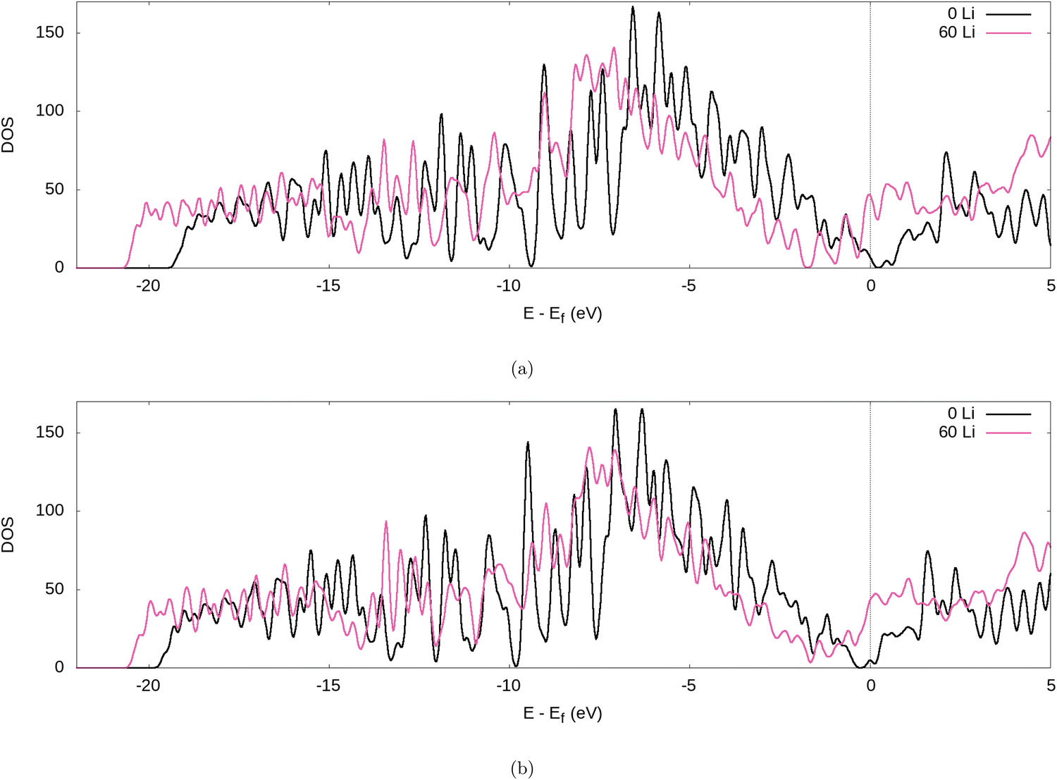 | ||
| Fig. 7 TDOS of the graphite nanoparticle compared to the fully lithiated graphite nanoparticle, for our (a) PBE-D2 and (b) optPBE calculations. | ||
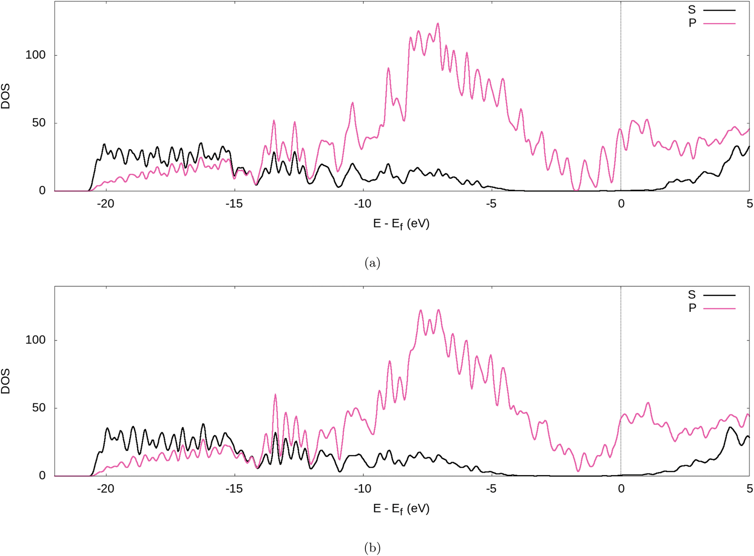 | ||
| Fig. 8 PDOS of the fully lithiated graphite nanoparticle, for our (a) PBE-D2 and (b) optPBE calculations. | ||
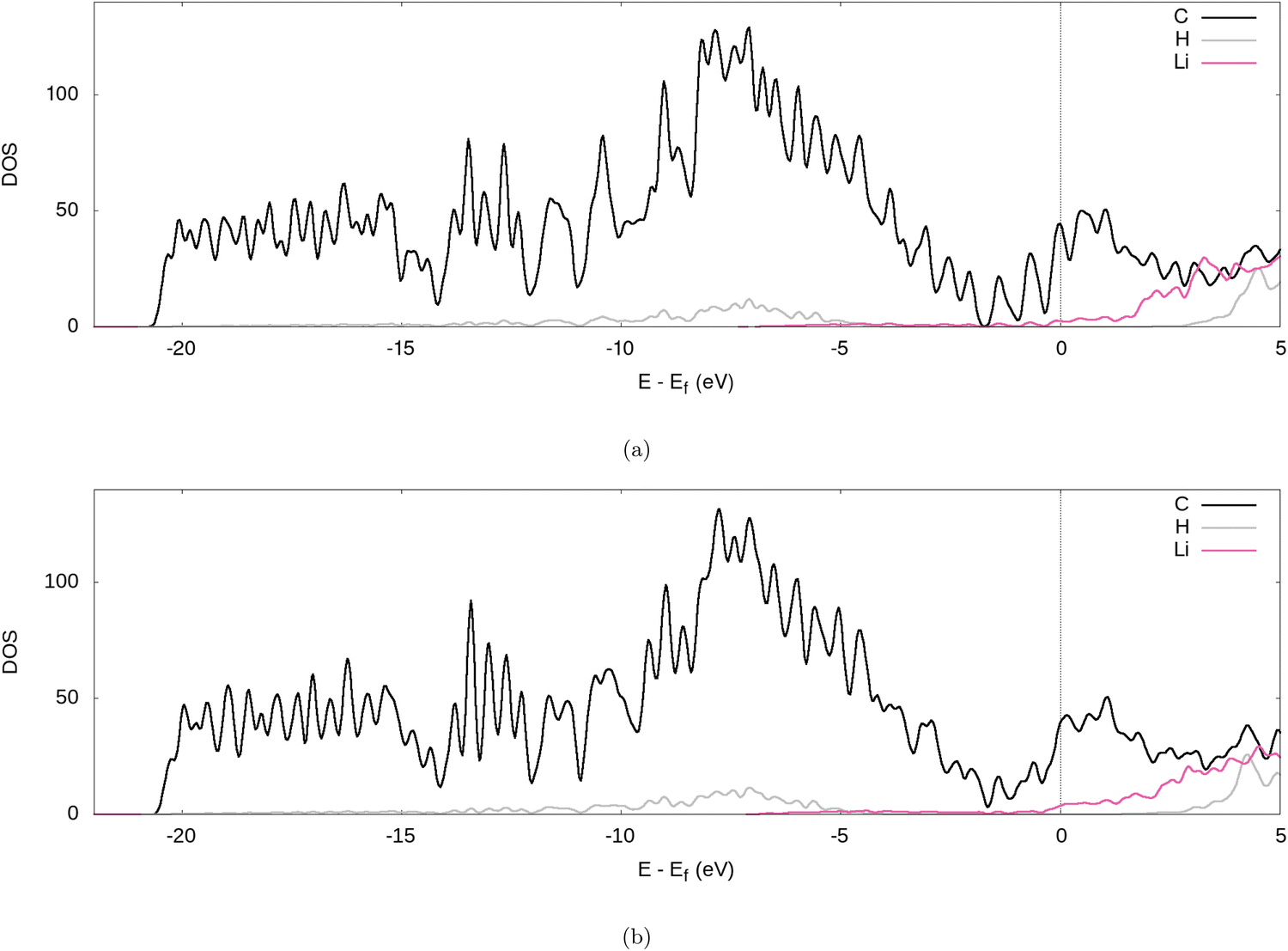 | ||
| Fig. 9 LDOS of the fully lithiated graphite nanoparticle, for our (a) PBE-D2 and (b) optPBE calculations. | ||
These findings are supported by previous theoretical studies on bulk graphite90–92 and experimental studies.11 The experimental findings of Mathiesen et al. went on to associate the charge transfer with the elongation of the interlayer carbon interactions and subsequent staging processes.11 Something we observe in our structure (cf. Section 3.1).
3.4 Voltage step profiles
We can directly compare the results of the intercalation procedure to that of experiment by computing a thermodynamically relevant observable quantity, the intercalation voltage. The Li intercalation reaction into the graphite nanoparticle, G, can be written as| nLi + G → LinG, | (2) |
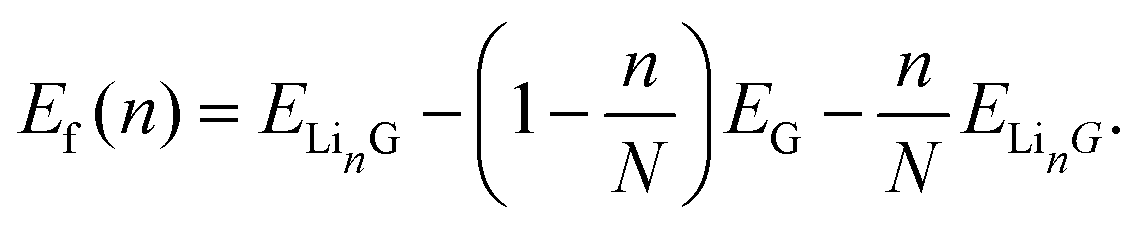 | (3) |
Here E is the DFT calculated energy. We can ignore the contributions of entropy at 0 K, while Pressure-volume contributions are also expected to be small.19,93–95 The calculated formation energy (Ef) is shown in Fig. 10a and b for the geometry optimized structures. We draw the convex hull using the convex hull finder Qhull.96
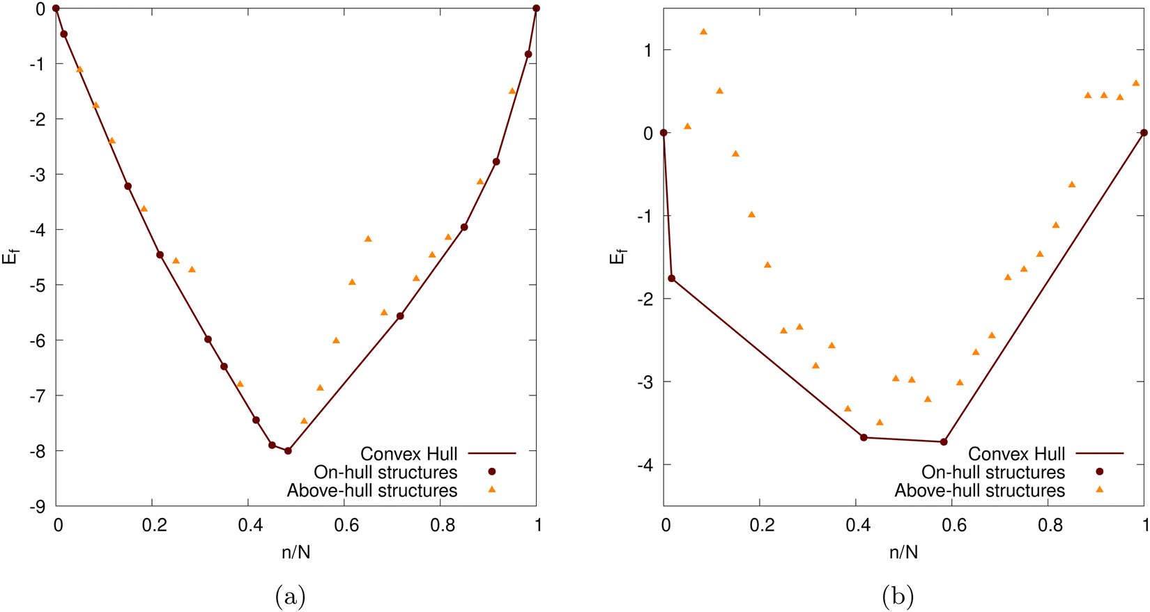 | ||
| Fig. 10 The formation energy of the Li intercalated graphite nanoparticles as a function of the degree of lithiation (n/N). N = 60 for our graphite nanoparticle, cf. Section 2.5 The Li intercalation proceeds via the convex hull (shown as brown line). The points on the convex hull (shown as brown circles) are the ground-states. The structures above the convex hull are shown with yellow triangles. Two different DFT functionals are considered: (a) PBE-D2 and (b) optPBE. | ||
The Li intercalation process proceeds along the convex hull via the identified ground-state structures. The intercalation reaction from a ground-state with n1 Li to the next ground-state with n2 Li can be written as
| (n2 − n1)Li + Lin1G → Lin2G. | (4) |
The intercalation voltage produced during this intercalation step from n1 to n2 can be calculated from the Nernst equation:95
 | (5) |
The intercalation voltage step profile is shown in Fig. 11 for both considered DFT functionals. PBE-D2 and optPBE nanoparticles vary in terms of shape and voltage range. With PBE-D2's profile occurring between approximately −0.4 and 0.9 V and optPBE's between approximately −0.2 and 1.75. The PBE-D2 voltage step profile has a very shallow initial step of about 0.2 V, whereas optPBE has an initial step of about 1.7 V. Both share an approximate plateau between 0.0 and 0.4 n/N. PBE-D2 has a drop just before 0.5 n/N before consistently decreasing. optPBE has two shallow drops in voltage occurring at around 0.4 and 0.6 n/N before plateauing. The PBE-D2 voltage step profile eventually decreases below 0 V at the around 0.9 n/N. For optPBE the drop below 0 V occurs much earlier at around 0.4 n/N. The drop below 0 V indicates that it has no longer become thermodynamically favourable for Li to intercalate into the nanoparticle at the position of lowest electrostatic potential.
 | ||
| Fig. 11 The computed Li intercalation voltage step profiles using two DFT functionals: PBE-D2 and optPBE. | ||
Given that our nanoparticle, when intercalated using both functionals, becomes saturated before reaching the theoretical maximum, discussed in Section 2.3, we could elect to stop the intercalation as soon as intercalation becomes unfavourable. This is a more ‘natural’ method of determining our nanoparticle's Li capacity. We visualise this in Fig. 12. Where N0 is the number of Li atoms present in the on-hull structure that upon intercalation results in a negative intercalation voltage. A more intuitive visualisation for the insertion energies of on-hull structures is given in our ESI.† For PBE-D2 the central decrease caused by the stage II to stage I transition is moved forward and more inline with that of experiment (cf.Fig. 13b). For optPBE the result of this new saturation limit is less clear due to the lack of on-hull structures generated in Fig. 13b. For this reason we will use the theoretical maximum as our intercalation limit so we can see how the voltage, beyond the thermodynamically unfavourable limit, evolves. We acknowledge that this means comparisons between experiment and our structure may not be as direct but we still believe they have value, particularly when comparing Li arrangements inside the nanoparticle.
 | ||
| Fig. 12 The computed Li intercalation voltage step profiles, where intercalation stops once it becomes thermodynamically unfavourable, using two DFT functionals: PBE-D2 and optPBE. | ||
 | ||
| Fig. 13 (a) A comparison of computational voltage step profiles with increasing lithiation adapted from references: Persson et al.,18 Mercer et al.,19Hazrati et al.,16 Pande and Viswanathan,97 Raju et al.,98 (b) a comparison of experimentally determined OCVs with increasing lithiation adaption from references: Ecker et al.,99 Mercer et al.,19 Allart et al.,27 Reynier et al.,10 Thomas and Newman.100 | ||
Other computational results that have focused on the bulk graphite are shown in Fig. 13a and are compared to our nanoparticle results. Even when modelling bulk graphite, computational voltage step profiles appear to vary extensively in magnitude and shape. Several factors affect the plots in such a way such as the selection of a different pseudopotential, dispersion corrections, and the exchange–correlation functionals.
We also compare our results with experimentally observed open circuit voltage (OCV) profiles in Fig. 13b. We note that PBE-D2 produces a voltage step profile that typically results in more favourable intercalations than that of experiment until the nanoparticle becomes saturated (i.e. when the voltage step profile becomes negative). Our PBE-D2 nanoparticle's voltage step profile's shape is also different from that of experimental OCVs (Fig. 13b). Some parallels can be drawn in terms of curve shape, such as the plateaus in both occurring around 0.1 to 0.5 n/N. The dip that occurs around 0.5 n/N in our PBE-D2 voltage step profile corresponds to the stage II to stage I transition is also present in experimental results. However, little resemblance can be observed beyond this point. Experimental results predict a plateau above 0.6 n/N whereas our PBE-D2 nanoparticle results continue to decrease. In comparison, our optPBE results predict a less favourable intercalation beyond the first intercalation with respect to experiment. According to this profile, it is apparent that optPBE predicts no favourable intercalation for this structure beyond the 0.4 n/N lithiation. When comparing the shape of this profile to that of experiment we see that the plateaus occurring at around 0.1 to 0.5 n/N are loosely replicated, the decrease at 0.6 n/N and the plateau from 0.5 to 1 are replicated well. We can conclude from this comparison that there is a significant difference between intercalation behaviour in our nanoparticle and that of bulk scale charging of an experimental anode. We can also conclude that, with the methodology we implement, the choice of functional has a large impact on the intercalation voltage, either through the geometry of the structure they produce or their energetic interpretation of such structures, and a careful selection will need to be made in future work.
The differences between experimental plots and our nanoparticle results can, in part, be explained by the increased ratio of terminated C atoms in our system compared that of a larger, more realistic nanoparticle. Indeed, it has been shown in a number of theoretical studies that an increased H atom to C atom ratio has a noticeable effect on binding energy.76,77,101 Given the well-documented sensitivity of the Li intercalation process to the interlayer binding of graphite, deviations are to be expected. We would also expect an experimental OCV to be effected by some of the different environmental factors such as having the experiment be performed at 298.15 K, the use of highly ordered pyrolytic graphite (HOPG), being mixed with carbon binder, being in a functioning lithium half-cell, or being in the presence of a mixture of ethylene carbonate and dimethyl carbonate as electrolyte which leads to the eventual formation of a solid electrolyte interphase (SEI). Whereas, our simulations occur in a vacuum, for a single nanoparticle of graphite, at 0 K and therefore would not exhibit any environmental effects. Another source of potential error is non-local DFT's known issue with modelling highly polarizable ions such as Li102 due to the use of atomic rather than ionic volumes.103 Anniés et al.104 identify this issue for Pande and Viswanathan's97 DFT-based Ising model which performs well for low Li abundance stages but not for high Li abundance stages. Further advancements can be made by considering graphite nanoparticles in electrolyte environments at applied voltage as in experimental electrochemistry. In the recent years, we have developed computational models for performing DFT simulations in electrolyte under potential control which could be the next step in this direction.105–107
3.5 AB pinning
As we report in Section 3.1, we observe no shift from an AB to an AA structure in our graphite nanoparticle as it is lithiated, something that we would expect to occur in a graphite-like compound. To investigate the cause of this lack of structural change we compare the energies of AA structures against that of AB structures. We compare the relative energies of the completely unfilled and completely filled nanoparticle with ideal Li spacing, Li42G (cf. Section 2.3).All calculations were performed with the parameters described in Section 2.3 using the optPBE exchange–correlation functional. All structures were relaxed using geometry optimisation.
The results in Table 2 show that for the empty graphite nanoparticle structure, the AB structure is 4.6 meV per atom lower in energy than the AA structure. This is expected given that the AB structure of graphite is lower in energy than that of AA graphite.43 We also note that for the comparison of the filled nanoparticle with perfect Li spacing the AB structure is 5.2 meV per atom higher in energy than the AA structure. This is also expected as full GICs are typically lower in energy in the AA configuration.43
| 592 atom nanoparticle | |||||
|---|---|---|---|---|---|
| Structure | AB 0 Li | AA 0 Li | AB 42 Li electrostatically distributed | AB 42 Li perfectly distributed | AA 42 Li perfectly distributed |
| eV per atom | −131.0469 | −131.0423 | −136.0106 | −136.0168 | −136.0220 |
Attention should be drawn to the nanoparticle filled with perfectly spaced Li is 6.2 meV per atom lower in energy than the filled nanoparticle with Li spacing generated by our method of intercalation (cf. Section 2.4). This is also to be expected given that we only use electrostatic potential as a guide for low energy sites and not as a definitive global minimum.
Given that the perfectly filled AB structure was relaxed with a geometry optimisation and it remained in the AB configuration, we can conclude that there is a local energy minimum for this carbon configuration. It is unclear whether the energy barrier to transition to from the AB structure to the AA is significant. Mercer et al.19 perform climbing image nudged elastic band calculations on this transition for bulk graphite and find no significant energy barrier. However, they do find meta-stable carbon sheet stackings as we do. They attribute their meta-stable stackings to the increased configuration entropy particularly present during de-lithiation caused by residual Li left in stage II ‘empty’ interlayer spaces. Our meta-stable states instead occur during lithiation where AB does not transition to AA. We can not attribute this to the increased configurational entropy of our system as a purely stage II AB structure is observed well beyond the expected lithiation limit for the transition to AA to occur (i.e. no ‘residual’ Li atoms are present in the empty layer until well beyond the point we would expect the AB to AA transition to occur). Of course, our calculations are performed at 0 K and we acknowledge there may be other entropic contributions that would destabilise our AB structure, such as the Li moving away from the edge. This leaves the geometry of our structure causing a significant energy barrier to transition from AB to AA as our leading explanation. Li–C binding at graphite edges has been reported to be stronger than Li–C binding in the bulk.34,108,109 Given the edge site presence of our structure, enhanced Li–C binding could cause an energy barrier to transition that is not present in bulk graphite.
In support of this explanation, we note that due to the way Li is distributed in the nanoparticle we made using our method, deformation in the graphite structure occurs that would allow for closer, central, inter-layer C–C bonds. Furthermore, the edge-favouring distribution of Li means that shifting layers would leave some Li atoms outside the nanoparticle which would either lead to a higher total energy due to the loss of enhanced edge Li–C interactions, if the atoms were to remain outside the particle, or would require a large Li atom reorganisation which will not occur without including a way of modelling the kinetics of Li during intercalation.
Therefore we believe that no AB to AA shift is observed in our structure as we intercalate with Li due to the local minimum AB being stabilised by the emptier outer intercalation layers and Li edge preference allowing the graphite sheets to flare and interact as if they were unintercalated as well as the possible AA structure being destabilised through edge accumulation meaning that an AA transition would lead to large scale deintercalaiton. This effect is allowed to occur because we provide no mechanism through which the Li can move and reorganise themselves. Unlike Mercer et al.19 reported meta stable structures delaying the transition of AA to AB we are likely observing a kinetic trap where Li not having the energy to diffuse through the graphite structure at this temperature means that the AB structure is pinned as the most stable state for this arrangement of Li.
4 Conclusions
In this study, we have demonstrated the feasibility of performing multiple ab initio calculations on entire graphite nanoparticles at various stages of charge. We also demonstrated a novel intercalation method whereby lithiation is dictated by the electrostatic global minimum. This method provides a suitable alternative to other intercalation schemes such as cluster expansion,18 with the advantage of being applicable to systems without long-range symmetry such as nanoparticles. Despite drastic structural and environmental differences of our nanoparticle to that of experiments, Li staging, Li to C charge transfer, and the formation of an OCV-like voltage step profile all occur readily. However, our nanoparticle results diverge from that of other bulk graphite results due to a preference for intercalation occurring at the edge sites. We believe the edge site preference is caused by the slight polarisation of edge C atoms by the more electropositive H atom terminations, which consequently creates an electrostatic potential minimum. The effect of this Li distribution is shown in the distribution of local charges and leads to an increased polarisation of the outer C atoms as more Li to C charge transfer occurs. We also found the edge accumulation of Li to be a likely cause of the nanoparticle structure being unable to transition from an AB to an AA configuration.Going forward, the availability of linear-scaling DFT we will be able to make more realistic atomistic models of intercalation. The same technique demonstrated here can be used in the future for more sophisticated models. These improvements could include structural refinements to our nanoparticle such as increased scale and edge terminations that better reflect a battery environment. Improvements to the model could include the inclusion of temperature-dependent Li intercalation, the addition of a kinetic model to our Li atoms that would enable them to diffuse through graphite and away from the edges, and the use of a solvent and electrolyte model.105–107
Conflicts of interest
There are no conflicts to declare.Acknowledgements
We would like to thank Louis Burgess, Thomas Ellaby, Rebecca Clements and Gabriel Bramley for advice and resources for processing the electrostatic potential. We also thank Dr Michael Mercer from the University of Lancaster and Dr Chiara Panosetti from Technische Universität München for directing us to some very useful sources of relevent literature. We are grateful to the UK Materials and Molecular Modelling Hub for computational resources, which is partially funded by EPSRC (EP/P020194/1 and EP/T022213/1). The authors acknowledge the use of the IRIDIS High Performance Computing Facility, and associated support services at the University of Southampton, in the completion of this work. This work used the ARCHER2 UK National Supercomputing Service (https://www.archer2.ac.uk). J. H. would like to thank BIOVIA for an EPSRC iCASE PhD funding. A. B. would like to thank the Faraday Institution (http://www.faraday.ac.uk; EP/S003053/1), grant numbers FIRG003 and FIRG025 for postdoctoral funding.References
- M. Armand and J.-M. Tarascon, Nature, 2008, 451, 652–657 CrossRef CAS PubMed
.
- B. Simon, S. Flandrois, K. Guerin, A. Fevrier-Bouvier, I. Teulat and P. Biensan, J. Power Sources, 1999, 81-82, 312–316 CrossRef CAS
- R. Fu, X. Zhou, H. Fan, D. Blaisdell, A. Jagadale, X. Zhang and R. Xiong, Energies, 2017, 10, 2174 CrossRef
- C. M. Hayner, X. Zhao and H. H. Kung, Annu. Rev. Chem. Biomol. Eng., 2012, 3, 445–471 CrossRef CAS
- W. A. V. Schalkwijk and B. Scrosati, Adv. Lithium-Ion Batteries, 2002, 1–5 Search PubMed
- N. A. Kaskhedikar and J. Maier, Adv. Mater., 2009, 21, 2664–2680 CrossRef CAS
- H. Zhang, Y. Yang, D. Ren, L. Wang and X. He, Energy Storage Mater., 2021, 36, 147–170 CrossRef
-
K. E. Thomas, J. Newman and R. M. Darling, in Advances in Lithium-Ion Batteries, ed. W. A. van Schalkwijk and B. Scrosati, Springer US, Boston, MA, 2002, pp. 345–392 Search PubMed
- M. S. Dresselhaus and G. Dresselhaus, Adv. Phys., 1981, 51, 1–186 CrossRef
- Y. Reynier, R. Yazami and B. Fultz, J. Power Sources, 2003, 119-121, 850–855 CrossRef CAS
- J. K. Mathiesen, R. E. Johnsen, A. S. Blennow and P. Norby, Carbon, 2019, 153, 347–354 CrossRef CAS
- A. Schleede and M. Wellmann, Z. Phys. Chem., 1932, 18, 1–28 Search PubMed
- K. C. Woo, H. Mertwoy, J. E. Fischer, W. A. Kamitakahara and D. S. Robinson, Phys. Rev. B: Condens. Matter Mater. Phys., 1983, 27, 7831–7834 CrossRef CAS
- K. C. Woo, W. A. Kamitakahara, D. P. Divincenzo, D. S. Robinson, H. Mertwoy, J. W. Milliken and J. E. Fischer, Phys. Rev. Lett., 1983, 50, 182–185 CrossRef CAS
- X. Chen, F. Tian, C. Persson, W. Duan and N.-X. Chen, Sci. Rep., 2013, 3, 3046 CrossRef
- E. Hazrati, G. A. de Wijs and G. Brocks, Phys. Rev. B: Condens. Matter Mater. Phys., 2014, 90, 155448 CrossRef
- M. P. Mercer, M. Otero, M. Ferrer-Huerta, A. Sigal, D. E. Barraco, H. E. Hoster and E. P. Leiva, Electrochim. Acta, 2019, 324, 134774 CrossRef CAS
- K. Persson, Y. Hinuma, Y. S. Meng, A. Van der Ven and G. Ceder, Phys. Rev. B: Condens. Matter Mater. Phys., 2010, 82, 125416 CrossRef
- M. P. Mercer, C. Peng, C. Soares, H. E. Hoster and D. Kramer, J. Mater. Chem. A, 2021, 9, 492–504 RSC
- E. M. Gavilán-Arriazu, O. A. Pinto, B. A. López de Mishima, D. E. Barraco, O. A. Oviedo and E. P. Leiva, Electrochem. Commun., 2018, 93, 133–137 CrossRef
- E. M. Perassi and E. P. Leiva, Electrochem. Commun., 2016, 65, 48–52 CrossRef CAS
- Y.-X. Yu, J. Mater. Chem. A, 2013, 1, 13559 RSC
- T. Han, Y. Liu, X. Lv and F. Li, Phys. Chem. Chem. Phys., 2022, 24, 10712–10716 RSC
- Y.-X. Yu, Phys. Chem. Chem. Phys., 2013, 15, 16819 RSC
- J. R. Dahn, Phys. Rev. B: Condens. Matter Mater. Phys., 1991, 44, 9170–9177 CrossRef CAS PubMed
- A. Senyshyn, O. Dolotko, M. J. Mühlbauer, K. Nikolowski, H. Fuess and H. Ehrenberg, J. Electrochem. Soc., 2013, 160, A3198–A3205 CrossRef CAS
- D. Allart, M. Montaru and H. Gualous, J. Electrochem. Soc., 2018, 165, A380–A387 CrossRef CAS
- D. A. Stevens and J. R. Dahn, J. Electrochem. Soc., 2001, 148, A803 CrossRef CAS
- F. Röder, S. Sonntag, D. Schröder and U. Krewer, Energy Technol., 2016, 4, 1588–1597 CrossRef
- O. E. Andersson, B. L. V. Prasad, H. Sato, T. Enoki, Y. Hishiyama, Y. Kaburagi, M. Yoshikawa and S. Bandow, Phys. Rev. B: Condens. Matter Mater. Phys., 1998, 58, 16387–16395 CrossRef CAS
- J. Vetter, P. Novák, M. R. Wagner, C. Veit, K. C. Möller, J. O. Besenhard, M. Winter, M. Wohlfahrt-Mehrens, C. Vogler and A. Hammouche, J. Power Sources, 2005, 147, 269–281 CrossRef CAS
- K. Takahashi and V. Srinivasan, J. Electrochem. Soc., 2015, 162, A635–A645 CrossRef CAS
- J. C. A. Prentice, J. Aarons, J. C. Womack, A. E. A. Allen, L. Andrinopoulos, L. Anton, R. A. Bell, A. Bhandari, G. A. Bramley, R. J. Charlton, R. J. Clements, D. J. Cole, G. Constantinescu, F. Corsetti, S. M. Dubois, K. K. B. Duff, J. M. Escartín, A. Greco, Q. Hill, L. P. Lee, E. Linscott, D. D. O'Regan, M. J. S. Phipps, L. E. Ratcliff, Á. R. Serrano, E. W. Tait, G. Teobaldi, V. Vitale, N. Yeung, T. J. Zuehlsdorff, J. Dziedzic, P. D. Haynes, N. D. M. Hine, A. A. Mostofi, M. C. Payne and C.-K. Skylaris, J. Chem. Phys., 2020, 152, 174111 CrossRef CAS
- C. Peng, M. P. Mercer, C. K. Skylaris and D. Kramer, J. Mater. Chem. A, 2020, 8, 7947–7955 RSC
- C. Peng, A. Bhandari, J. Dziedzic, J. R. Owen, C.-K. Skylaris and D. Kramer, J. Mater. Chem. A, 2021, 33, 45–47 Search PubMed
- A. Bhandari, C. Peng, J. Dziedzic, J. R. Owen, D. Kramer and C.-K. Skylaris, J. Mater. Chem. A, 2022, 10, 11426–11436 RSC
- G. Ceder, Comput. Mater. Sci., 1993, 1, 144–150 CrossRef CAS
- Y. Ran, Z. Zou, B. Liu, D. Wang, B. Pu, P. Mi, W. Shi, Y. Li, B. He, Z. Lu, X. Lu, B. Li and S. Shi, npj Comput. Mater., 2021, 7, 184 CrossRef CAS
- A. Van der Ven, M. K. Aydinol, G. Ceder, G. Kresse and J. Hafner, Phys. Rev. B: Condens. Matter Mater. Phys., 1998, 58, 2975–2987 CrossRef CAS
-
C. M. Wolverton, PhD thesis, University of California Berkley, 1993
- J. X. Shen, M. Horton and K. A. Persson, npj Comput. Mater., 2020, 6, 161 CrossRef CAS
- S. A. Safran, Solid State Phys., 1987, 40, 183–246 CAS
- Y. Imai and A. Watanabe, J. Alloys Compd., 2007, 439, 258–267 CrossRef CAS
- F. Wang, J. Graetz, M. S. Moreno, C. Ma, L. Wu, V. Volkov and Y. Zhu, ACS Nano, 2011, 5, 1190–1197 CrossRef CAS PubMed
- C.-K. Skylaris, P. D. Haynes, A. A. Mostofi and M. C. Payne, J. Chem. Phys., 2005, 122, 084119 CrossRef PubMed
- C.-K. Skylaris, A. A. Mostofi, P. D. Haynes, O. Diéguez and M. C. Payne, Phys. Rev. B: Condens. Matter Mater. Phys., 2002, 66, 035119 CrossRef
- A. A. Mostofi, P. D. Haynes, C.-K. Skylaris and M. C. Payne, J. Chem. Phys., 2003, 119, 8842–8848 CrossRef CAS
- D. C. Langreth, M. Dion, H. Rydberg, E. Schröder, P. Hyldgaard and B. I. Lundqvist, Int. J. Quantum Chem., 2005, 101, 599–610 CrossRef CAS
- P. Hobza, J. Poner and T. Reschel, J. Comput. Chem., 1995, 16, 1315–1325 CrossRef CAS
- M. J. Allen and D. J. Tozer, J. Chem. Phys., 2002, 117, 11113–11120 CrossRef CAS
- S. Kristyán and P. Pulay, Chem. Phys. Lett., 1994, 229, 175–180 CrossRef
- T. Gould, S. Lebègue and J. F. Dobson, J. Phys.: Condens. Matter, 2013, 25, 445010 CrossRef
- R. Sabatini, T. Gorni and S. De, Gironcoli, Phys. Rev. B: Condens. Matter Mater. Phys., 2013, 87, 4–7 CrossRef
- T. Björkman, Phys. Rev. B: Condens. Matter Mater. Phys., 2012, 86, 165109 CrossRef
- M. Dion, H. Rydberg, E. Schröder, D. C. Langreth and B. I. Lundqvist, Phys. Rev. Lett., 2004, 92, 246401 CrossRef CAS
- K. Lee, É. D. Murray, L. Kong, B. I. Lundqvist and D. C. Langreth, Phys. Rev. B: Condens. Matter Mater. Phys., 2010, 82, 081101 CrossRef
- J. Klimeš, D. R. Bowler and A. Michaelides, J. Phys.: Condens. Matter, 2010, 22, 022201 CrossRef
- S. Grimme, J. Comput. Chem., 2006, 27, 1787–1799 CrossRef CAS PubMed
- A. Tkatchenko and M. Scheffler, Phys. Rev. Lett., 2009, 102, 6–9 CrossRef PubMed
- S. Grimme, J. Antony, S. Ehrlich and H. Krieg, J. Chem. Phys., 2010, 132, 154104 CrossRef PubMed
- S. Grimme, S. Ehrlich and L. Goerigk, J. Comput. Chem., 2011, 32, 1456–1465 CrossRef CAS
- E. Caldeweyher, C. Bannwarth and S. Grimme, J. Chem. Phys., 2017, 147, 034112 CrossRef PubMed
- G. Bramley, M.-T. Nguyen, V.-A. Glezakou, R. Rousseau and C.-K. Skylaris, J. Chem. Theory Comput., 2020, 16, 2703–2715 CrossRef CAS
- N. C. Siersch, T. B. Ballaran, L. Uenver-Thiele and A. B. Woodland, Am. Mineral., 2017, 102, 845–850 CrossRef
- C. K. Skylaris and P. D. Haynes, J. Chem. Phys., 2007, 127, 6–11 CrossRef
- F. Birch, Phys. Rev., 1947, 71, 809–824 CrossRef CAS
- F. D. Murnaghan, Proc. Natl. Acad. Sci. U.
S. A., 1944, 30, 244–247 CrossRef CAS
- Y. Baskin and L. Meyer, Phys. Rev., 1955, 100, 544 CrossRef CAS
- R. Zacharia, H. Ulbricht and T. Hertel, Phys. Rev. B: Condens. Matter Mater. Phys., 2004, 69, 155406 CrossRef
- Z. Liu, J. Z. Liu, Y. Cheng, Z. Li, L. Wang and Q. Zheng, Phys. Rev. B: Condens. Matter Mater. Phys., 2012, 85, 205418 CrossRef
-
L. X. Benedict, N. G. Chopra, M. L. Cohen, A. Zettl, S. G. Louie and V. H. Crespi, CHEMICAL PHYSICS LETTERS ELSEVIER Microscopic determination of the interlayer binding energy in graphite, 1998 Search PubMed
- O. Lenchuk, P. Adelhelm and D. Mollenhauer, J. Comput. Chem., 2019, 40, 2400–2412 CrossRef CAS
- J. P. Perdew, K. Burke and M. Ernzerhof, Phys. Rev. Lett., 1996, 77, 3865–3868 CrossRef CAS
- G. Kresse and J. Furthmüller, Comput. Mater. Sci., 1996, 6, 15–50 CrossRef CAS
- BIOVIA, Dassault Systemes, Materials Studio, 20.1.0.5, San Diego: Dassault Systemes, 2020
- T. S. Totton, A. J. Misquitta and M. Kraft, J. Phys. Chem. A, 2011, 115, 13684–13693 CrossRef CAS PubMed
- A. James and R. S. Swathi, J. Phys. Chem. A, 2022, 126, 3472–3485 CrossRef CAS PubMed
- E. Lee and K. A. Persson, Nano Lett., 2012, 12, 4624–4628 CrossRef CAS
- P. E. Blöchl, Phys. Rev. B: Condens. Matter Mater. Phys., 1994, 50, 17953–17979 CrossRef PubMed
- J. W. Bennett, B. G. Hudson, I. K. Metz, D. Liang, S. Spurgeon, Q. Cui and S. E. Mason, Comput. Mater. Sci., 2019, 170, 109137 CrossRef CAS
- K. F. Garrity, J. W. Bennett, K. M. Rabe and D. Vanderbilt, Comput. Mater. Sci., 2014, 81, 446–452 CrossRef CAS
- Á. Ruiz-Serrano and C.-K. Skylaris, J. Chem. Phys., 2013, 139, 054107 CrossRef PubMed
- D. F. Shanno, Math. Oper. Res., 1978, 3, 244–256 CrossRef
- N. D. Hine, J. Dziedzic, P. D. Haynes and C. K. Skylaris, J. Chem. Phys., 2011, 135, 1–18 CrossRef PubMed
- V. Chevrier and J. R. Dahn, J. Electrochem. Soc., 2009, 156, A454 CrossRef CAS
- D. R. Baker and M. W. Verbrugge, J. Electrochem. Soc., 2020, 167, 013504 CrossRef CAS
- M. Kühne, F. Börrnert, S. Fecher, M. Ghorbani-Asl, J. Biskupek, D. Samuelis, A. V. Krasheninnikov, U. Kaiser and J. H. Smet, Nature, 2018, 564, 234–239 CrossRef
- X. Y. Song, K. Kinoshita and T. D. Tran, J. Electrochem. Soc., 1996, 143, L120–L123 CrossRef CAS
- R. S. Mulliken, J. Chem. Phys., 1955, 23, 1833–1840 CrossRef CAS
- N. A. W. Holzwarth, S. G. Louie and S. Rabii, Phys. Rev. B: Condens. Matter Mater. Phys., 1984, 30, 2219–2222 CrossRef CAS
- C. Hartwigsen, W. Witschel and E. Spohr, Phys. Rev. B: Condens. Matter Mater. Phys., 1997, 55, 4953–4959 CrossRef CAS
-
H. Zabel, Graphite Intercalation Compounds II: Transport and Electronic Properties, Springer Berlin Heidelberg, Berlin, Heidelberg, 1992 Search PubMed
- Y. Reynier, J. Graetz, T. Swan-Wood, P. Rez, R. Yazami and B. Fultz, Phys. Rev. B: Condens. Matter Mater. Phys., 2004, 70, 174304 CrossRef
- E. B. Isaacs, S. Patel and C. Wolverton, Prediction of Li intercalation voltages in rechargeable battery cathode materials: effects of exchange-correlation functional, van der Waals interactions, and Hubbard U, 2020.
- M. K. Aydinol, A. F. Kohan and G. Ceder, J. Power Sources, 1997, 68, 664–668 CrossRef CAS
- C. B. Barber, D. P. Dobkin and H. Huhdanpaa, ACM Trans. Math. Softw., 1996, 22, 469–483 CrossRef
- V. Pande and V. Viswanathan, Phys. Rev. Mater., 2018, 2, 1–10 Search PubMed
- M. Raju, P. Ganesh, P. R. Kent and A. C. Van Duin, J. Chem. Theory Comput., 2015, 11, 2156–2166 CrossRef CAS
- M. Ecker, T. K. D. Tran, P. Dechent, S. Käbitz, A. Warnecke and D. U. Sauer, J. Electrochem. Soc., 2015, 162, A1836–A1848 CrossRef CAS
- K. E. Thomas and J. Newman, J. Power Sources, 2003, 119-121, 844–849 CrossRef CAS
- B. Li, P. Ou, Y. Wei, X. Zhang and J. Song, Materials, 2018, 11, 726 CrossRef
- T. Bučko, S. Lebègue, J. Hafner and J. G. Ángyán, Phys. Rev. B: Condens. Matter Mater. Phys., 2013, 87, 064110 CrossRef
- T. Gould, S. Lebègue, J. G. Ángyán and T. Bučko, J. Chem. Theory Comput., 2016, 12, 5920–5930 CrossRef CAS PubMed
- S. Anniés, C. Panosetti, M. Voronenko, D. Mauth, C. Rahe and C. Scheurer, Materials, 2021, 14, 6633 CrossRef
- J. Dziedzic, A. Bhandari, L. Anton, C. Peng, J. C. Womack, M. Famili, D. Kramer and C.-K. Skylaris, J. Phys. Chem. C, 2020, 124, 7860–7872 CrossRef CAS
- A. Bhandari, L. Anton, J. Dziedzic, C. Peng, D. Kramer and C.-K. Skylaris, J. Chem. Phys., 2020, 153, 124101 CrossRef
- A. Bhandari, C. Peng, J. Dziedzic, L. Anton, J. R. Owen, D. Kramer and C.-K. Skylaris, J. Chem. Phys., 2021, 155, 024114 CrossRef CAS
- L. M. Morgan, M. P. Mercer, A. Bhandari, C. Peng, M. M. Islam, H. Yang, J. Holland, S. W. Coles, R. Sharpe, A. Walsh, B. J. Morgan, D. Kramer, M. S. Islam, H. E. Hoster, J. S. Edge and C.-K. Skylaris, Progress in Energy, 2022, 4, 012002 CrossRef
- E. G. Leggesse, C.-L. Chen and J.-C. Jiang, Carbon, 2016, 103, 209–216 CrossRef CAS
Footnote |
| † Electronic supplementary information (ESI) available: Our supporting information contains an image of our simulation cell with our nanoparticle inside, images of all structures we produce, further Mulliken population analysis, and a graph showing our insertion energies. We also include the associated output files with the Li intercalation calculations, which contains the necessary data and scripts to reproduce our results. See DOI: https://doi.org/10.1039/d2ma00857b |
| This journal is © The Royal Society of Chemistry 2022 |