
 Open Access Article
 This Open Access Article is licensed under a Creative Commons Attribution-Non Commercial 3.0 Unported Licence
Grow with the flow – observing the formation of rheotactically patterned bacterial cellulose networks†
Moritz
Klotz
 ,
Dardan
Bajrami
and
Daniel
Van Opdenbosch
*
,
Dardan
Bajrami
and
Daniel
Van Opdenbosch
*
Technical University of Munich, Campus Straubing for Biotechnology and Sustainability, Chair for Biogenic Polymers, Schulgasse 16, D-94315 Straubing, Germany. E-mail: moritz.klotz@tum.de
First published on 7th June 2022
Abstract
The use of matrix-forming organisms is a promising way to obtain hierarchically structured materials. In this work, we investigate the rheotactic bio-mediated alignment and network formation of bacterial cellulose streamers, resulting in hierarchically patterned textiles. For this purpose, we devised a panoramic-view observation setup for a microfluidic cell. We observed a split growth, with first, a flow-aligned streamer formation and second, a streamer connection phase. The growth phase parameters showed dependence on flow rate. After aligned growth, a mineralisation step was conducted to the grown textiles with calcium carbonate and -sulfate to obtain nature-inspired organic/inorganic composite materials. Hereby, an anisotropic deposition of the gypsum phase due to the prealigned bacterial cellulose substrate was observed.
1 Introduction
The growth of natural materials differs fundamentally from the production of engineering materials: while engineering materials’ requirements are typically fulfilled by choice of substance and shaping techniques, nature forms its materials from readily available elements into hierarchical structures.1 Hence, biological materials derive their widely varying properties mainly from the adaptation of internal structuring to meet functional requirements.2,3 The most prominent aspects hereof are hierarchical structure and structural anisotropy. In addition, dispersed polymer phases enable stress relaxation and structural regression of the material due to their viscoelasticity, sacrificial bonds and ‘hidden lengths’.4In order to obtain bio-mimetic mechanical properties in engineering materials, different approaches can be pursued: applying biomorphism and biotemplating, it is possible to convert a naturally grown template into an inorganic replica material retaining most, or all, of the hierarchical levels of structuring, leading to exciting mechanical properties.5–8 With some restrictions, it is also possible to obtain hierarchical structures by the self-organizing material synthesis in an artificial process.9 However, up-scaling these processes, which were reviewed by Deuerling et al. as ‘Level 1 – Transfer of structure’,10 to produce competitive engineering materials remains a challenge.
Nature, on the other hand, readily produces large-scale composite materials via hierarchical structuring. Therefore, bio-mediated material structuring, reviewed by Deuerling et al. as ‘Level 2 – Usage of biological systems’,10 offers the potential to control material formation from the micro to the macro level. Here, biological systems are influenced by stimuli to which the living cells and microbes react by movement, ‘taxis’. The growth into a certain culture medium as an internal stimulus,10 as well as the directed growth after external stimuli, e.g. light,11–13 mechanical influences14–17 and a variety of other attractants,18–20 can serve to create a biological, hierarchically structured template to be used for different purposes than intended by nature. The advantage of this approach is that biological materials are typically already hierarchically structured, starting at the molecular level: Biofilms, for example, are microorganisms embedded in their extracellular polymeric matrix (EPS).21 While they are undesirable in most living and technical systems, they feature a hierarchical structure.22,23 Specifically, bacterial cellulose biofilms (BCB) consisting mainly of bacterial cellulose (BC), exhibit several structural levels: starting from the cellulose molecules, the bacteria produce microfibrils at the nanometer level which consist of amorphous and crystalline regions. The microfibrils arrange into ribbons, building bundles, which then cluster into bacterial cellulose networks.24,25
Several works have considered bio-mediated structuring of BCB, respectively the BC fibers: Kondo et al. and Uraki et al. similarly used already-deposited cellulose strands as templates for further deposition.16,26 Anisotropic deposition of BC is possible by using nematic ordered cellulose (NOC) or stretched cellulose as templates.27,28 Also of interest is the alignment via growth on polydimethylsiloxane (PDMS) with a ridged morphology.29–31 By varying ridge sizes, Putra et al. archived a 2.3 times higher fracture stress and a 3.8 times lower elastic modulus, compared to air-grown BCB. His group was also able to produce mechanically anisotropic behavior with BCB grown in thin silicon tubes, as well as by influencing the culture interface via silicon oil.32,33 Also promising are the works of Sano et al. and Liu et al. who successfully used an electromagnetic field to align BCB.34,35
Wan et al. and Luo et al. carried out structuring by a flow approach: Wan et al. were able to align the BCB with the flow and increase the tensile strength in the BC fiber direction from 0.9 MPa to 1.2 MPa, while the fracture strain decreased by 8%. Luo et al. even achieved a tensile strength of 1.5 MPa with a flow velocity of 150 mm−1, with a fracture strain decrease of 12%.36,37 Using flow-producing rising bubbles, Chae et al. also attained a unidirectional deposition of BCB.38
Since structuring of BCB by flow has already yielded interesting results, it is worth considering the mechanism: if a biofilm grows in a flowing medium, its viscoelastic morphology responds to the mechanical stimulus of the flow.39 The form thereby differs if the biofilm is fully surface attached or if it adheres at least at one point, while the rest of the biofilm moves with the flow as a so-called streamer. The streamer formation and its physics have been studied by several research groups.40–43 As intuitively expected, the geometry and the flow velocities of the system have a great influence on the streamers’ shapes.15,44–47 Interestingly, whether streamers start to form is largely independent of the Reynolds number, as summarized by Karimi et al.41 The dynamics of the flow can also influence the growth system, as can be seen in experiments with pulsative or split flow.48,49 Condensed, the streamers morphology but also the strength of attachment are strongly influenced by their viscoelastic behavior50 which is a function of its structure. The structure formation in turn is influenced by the flow: in contrast to fish, copepods and some protists, which possess a receptor for flow forces and exhibit active rheotaxis, bacteria react in a passive way to the shear stress factor, comparable with other passive physical movement phenomena like gyro- and magnetotaxis.51 Bacterial rheotaxis is triggered by bacterial motility and morphology.52 While the swimming direction of motile bacteria is changed by torque, non-motile bacteria expand along their biofilm, due to the predominant shear forces under flow conditions.47,53 For BC producing bacteria, it is likely that extrusion of BC and cell division based fiber-anchoring24 provide this movement. Together with the morphology induced alignment, which occurs for ellipsoidal bacteria like Komagataeibacter xylinus (K. xylinus),37,50 we consider the flow based forming of the BCB as a type of rheotaxis. So far, rheotaxis and streamer formation has been studied mainly in single, isolated samples. The formation of streamer networks has been investigated rarely, and mainly with the aim of being able to avoid them, and the associated clogging of fluidic systems. Worth mentioning is the work by Hassanpourfard et al. who investigated fast-formed Pseudomonas fluorescens streamer-networks and found that they still moved by a viscoelastic ‘stick-slip’ dynamic, which allows the formation of channels, resulting in regions of varying density.54,55
In summary, the in situ structuring and alignment of biofilm streamers, in particular of BCB, can be realised by a variety of approaches. However, in order to produce engineering materials, processes have to be adapted to include larger-scale hierarchical structuring and outer shapes, such as honeycomb structures.16,26 At this point, rheotactic structuring has advantages: flow bodies can have any shape and size and there is a high degree of flexibility due to the large number of parameters such as flow, species and medium composition. Another advantage is the direct introduction of additives into the growth system, which allows the formation of organic/inorganic composite via an in situ or quasi in situ mineralisation route.
Generally, composites with BCB, respectively, BC as the substrate are of interest, especially for medical purposes, as the reviews from Shan et al. and Liu et al. illustrate. Mainly for the investigation of new tissue materials, dozens of BC combinations with polymers or nanomaterials were tested.56,57 Excellent mechanical properties were obtained by impregnation of the grown BC ex situ.58 However, in situ mineralisation by which the composites are produced during BCB growth, or quasi in situ mineralisation, where the BCB is treated in the same vessel directly after growth, are promising. Literature thereof, in the combination organic/inorganic, so far is limited to (nano)particle,59–61 fibers35,62 and minerals e.g. hydoxyapatite or clay.63–66 Inspired by biological materials with tough or self-healing properties like nacre,67 we assume that rather the latter combination is suitable to obtain a scalable, hierarchically and nature oriented engineering material. Materials which can be processed by a wet mineralisation route in a quasi in situ setup.
CaCO3/cellulose composites, serving as a model for quasi in situ mineralisation, can be achieved by different approaches, such as the already mentioned direct deposition of particles,59,60 or via the precipitation from precursors. The latter works via diffusive processes68 or faster, via direct mixing. The intermediate which occurs during the precipitation of CaCO3 is amorphous calcium carbonate (ACC), which can serve as the inorganic phase after stabilization69–71 or after crystallisation.72–75 ACC can be used in a one step process, without the need for a second reagent. Also a one step process is the deposition of gypsum from supersaturated solutions. Despite gypsum's low cost and the possibility to overcome drawbacks such as brittleness, gypsum/cellulose composites have not been the focus of many publications so far. However, due to the possibility of a one-step mineralisation and its typical acerous morphology, which lends itself to textured mineralisation, it is well suited for use with prealigned BCB. Gypsum mineralisation on a cellulose substrate was already achieved by Nissinen et al., who used supersaturated CaCl2–Na2SO4 solutions.76
Bio-mediated materials with hierarchical structures can be made by rheotactic approaches as demonstrated by Wan et al. and Luo et al.36,37 Building on these results, we aim to extend the fundamental knowledge of flow based material patterning for future upscaling and material production. Investigating the growth dynamics leads to an improved understanding of the rheotactic biofilm formation and enables prospective reproducible material production. We hypothesized that an initial homogeneous distribution of EPS-forming microbes on obstacles, positioned with a long-range order and subjected to volume-driven flow, will lead to their uniform growth, resulting in a network of streamers. The growth parameters thereby are a key aspect to tailor a well defined material with specific structural features on several hierarchical levels. Such a material can serve as a matrix for organic/inorganic composites whose hierarchical characteristics span its different phases. Therefore, we evaluated in a panoramic-view observation setup the obstacle-induced streamer and streamer-network formation of K. xylinus at three different flow rates. After growth, we assessed two potential mineralisation routes by a quasi in situ process: in a one step process either the amorphous precursor ACC or a supersaturated solution of CaSO4 was added directly into the growth chamber.
2 Experimental
2.1 Setup
Fig. 1 shows the experimental setup for the growth experiments. A batch culture (1) of K. xylinus was pumped by a syringe pump (2) through a pressure sensor (3) and a double bubble trap (4, 5) into a microfluidic cell (8) in a circular flow. Growth in the microfluidic cell was observed using an optical setup (6–10). | ||
| Fig. 1 Sketch of the experimental setup. The inoculum (1) of K. xylinus was taken from below the BCB pellicle by a syringe pump (2), injected via a pressure sensor (3) and a double bubble trap (4, 5) into the microfluidic cell (8), and recycled into the batch culture (1). The microfluidic cell was illuminated in transmission with nearly parallel light (7) emitted by a white LED (6). After passing an optional optical filter which allows schlieren techniques (9, not used in the current experiments), the observation took place using a camera (10). For clarity, the beam path is simplified. | ||
 | ||
| Fig. 2 Sketch of the microfluidic cell. The inoculum was injected into the larger inlet (1) from where it was evenly distributed into the inlet channels. This regularly allowed an even distribution of the fluid into the growth chamber, which was filled with evenly arranged obstacles with diameters of 50 μm in 0.5 mm distance. After the growth, the smaller inlet (2) was used to add mineralisation medium. The inset shows a magnified section of the growth chamber. | ||
2.2 Experimental procedure
For each of the three different flow rates, four repeating experiments were conducted at ambient temperature 21 ± 1 °C. The necessary volume flow for the mean flow rates of 1.0 mm s−1, 12.5 mm s−1 and 25.0 mm s−1 were calculated for the growth chamber of the microfluidic cell.Before each of the 12 experiments, all tubes (PTFE, inner diameter 1/32”), fittings and the second bubble trap were autoclaved. After assembly of the components, the setup was flushed with 20% H2O2 (Carl Roth, Karlsruhe, Germany) for one hour to sterilize all unautoclavable parts including the microfluidic cell, both bubble traps, the valve and the pressure sensor (CPS 2184 Z, 5 bar, CETONI, Korbussen, Germany).
At the start of an experiment, a syringe pump (neMESYS 290N with QmixElements, CETONI, Korbussen, Germany) equipped with a 3-2-way valve ((2) in Fig. 1), pumped inoculum from below the BCB pellicle in cycles through the microfluidic cell and back into the flask. During the experiments, which lasted up to 70 h, the syringes were automatically refilled. All pump parameters are listed in Table 1.
Since the long-lasting experiments were susceptible to air bubbles which degrade the grown biofilm, a double bubble trap ((4,5) Fig. 1) was used. The first (Bubble Trap for Microfluidics, ELVEFLOW, Paris, France) for large bubbles appearing in the starting phase and the second (Microfluidic Reservoir XS, ELVEFLOW, Paris, France), for small bubbles appearing during the experiments, which were not removable by the first trap. Additionally, the second bubble trap buffered pressure impulses and allowed a more even flow. With the pressure sensor, a servo loop was adjusted. The experiments were conducted until the slowly increasing pressure reached 1 bar and the servo loop started to minimize the flow rate from Table 1. For the evaluation, only the data before the start of the servo loop with the constant adjusted flow (below 1 bar) were used. To document the growth, 8-bit black/white images were recorded via Micro–Manager78 every 10 minutes.
After each experiment, the setup was flushed with 5–10 ml deionised water (DI) to remove all water-soluble substances. For this, the maximum pressure was step-wise increased, up to a maximum of 1.5 bar. After the following mineralisation steps which were conducted on some samples, the microfluidic cells were dried for 24 h at 45 °C and opened mechanically to obtain the biofilm.
2.3 Growth analysis
For determining ε, the biofilm thickness lBCB of one reference sample was obtained by breaking the sample after freezing in liquid nitrogen. lBCB then was determined by SEM at 19 measuring points at the fracture plane. We assume that the vacuum-dried BCB was contracted compact and dense with marginal interspaces. This is supported by the SEM images (see Fig. S3(d), ESI†). Since only BCB influenced light absorbance due to the use of the reference images at t0, we defined the reference mass concentration cref with the measured BCB density ρBCB by eqn (1). To measure ρBCB, in total 48 BCB pieces of six separate batch-grown samples were washed, dried at 65 °C and weighed. Afterwards, they were soaked for 24 h in DI water at <0.1 bar to remove embedded air. Their densities were determined by Archimedes’ principle (224-1S, Sotoris Entris, Göttingen, Germany) with a mean result of ρBCB = 1.12 ± 0.03 g cm−3.
 | (1) |
 | (2) |
 | (3) |
After conversion, the isolines of γ(cBCB,b, t) were fitted between 0 < γ ≤ 1 via a bi-logistic fit, which was performed by the least-squares algorithm of the Python lmfit package. With the maximum curve values S, the inflexion points Δt of the sigmoid curves and the logistic growth constants λ, fits were performed after eqn (4). The plots shown in this work ended when the fitted parameter of at least two measurements reached zero or unrealistic values.
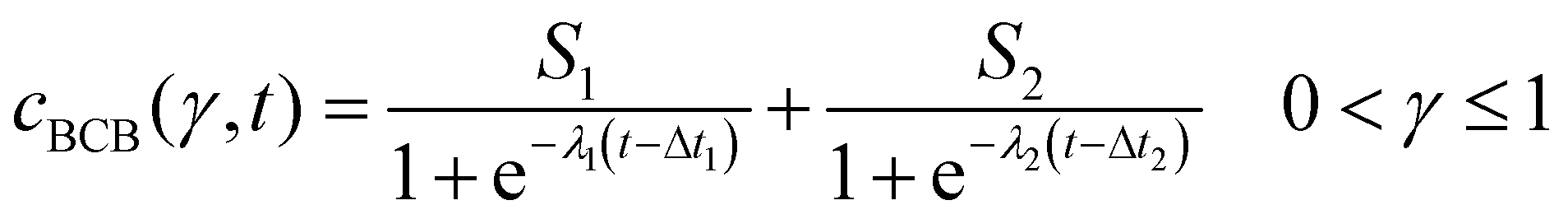 | (4) |
![[c with combining macron]](https://www.rsc.org/images/entities/i_char_0063_0304.gif) BCB(i,j,t) were calculated. For determining the concentration increase rates, the resulting mean data of the three flow rates were fitted by linear regression via the Python SciPy theilslopes Theil–Sen estimator.
BCB(i,j,t) were calculated. For determining the concentration increase rates, the resulting mean data of the three flow rates were fitted by linear regression via the Python SciPy theilslopes Theil–Sen estimator.
2.4 Flow simulation
Two-dimensional finite volume element simulation of the fluid flow (CFD) in the microfluidic cell without biofilm was performed with ANSYS FLUENT (Ansys, Pennsylvania, USA) for the three different flow rates. The defined working fluid was the culturing medium before inoculation (dynamic viscosity = 1.34 mPa s (Ubbelohde viscometer with a type 50103/0c capillary, SI Analytics, Mainz, Germany), density = 0.99 ± 0.01 g ml−1). As the flow rates and Reynolds numbers where low, the flow was considered incompressible, laminar and steady state. The system was set as isothermal, without any gravity effects and the boundary conditions at the walls were considered as non-slip and the pressure at the outlet as atmospheric. For the pressure-velocity linking, the coupled method was used. For discretisation, “second order upwind” was selected for pressure and momentum. The convergence criteria were set as 10−10 for all equations. For evaluation of the method, a grid independence study was performed, Fig. S6 (ESI†).2.5 Mineralisation
Mineralisation of biofilms was conducted by crystallisation of CaCO3 from ACC or CaSO4 from a supersaturated solution. For the CaCO3 mineralisation, the microfluidic cells, after they were flushed with water, were rinsed with 3 M CaCl2·2H2O (Th. Geyer, Renningen, Germany) solutions for at least one hour. Under a continuous flow of 1 μl s−1, the second inlet ((2) in Fig. 2) was first flushed with DI–water and then with a 3 M Na2CO3 (Carl Roth, Karlsruhe, Germany) solution manually injected by a syringe until the microfluidic cells clogged. The ACC precipitated directly in the growth chambers, where the ensuing mineralisation could be observed. After a rest period of about 17 h, the cells were flushed with at least 5 ml DI–water at a pressure up to 1.5 bar.For the CaSO4 mineralisation, solutions of 0.4 M CaCl2·2H2O and Na2SO4 (Carl Roth, Karlsruhe, Germany) were mixed and injected via a 0.2 μm syringe-filter into the cell inlets until the filter clogged after 1–2 ml solution. After a rest period of about 17 h, when no further mineralisation was observable, the cell was dried at 45 °C, without flushing. Preliminary tests showed that a supersaturated solution of this concentration stays stable for approximately four minutes before crystallisation initiates.
2.6 Metrology
For the assessment of biofilm mineralisation, the mineralised biofilms were measured for 10° < 2θ < 60° and 0.5° min−1 while being spun to equalize any in-plane texture. Additionally, they were measured in transmission mode (Item no: 2101G102, Rigaku, Tokyo, Japan) with the flow direction parallel to the scattering vector, at 2θ/2. The measuring speed was 0.1° min−1, with divergence Slit = 0.1 mm. Since in transmission mode the sample height equals the XRD beam diameter, sample-depended peak broadening and thus crystallite sizes could only be obtained for the rotating in-plane measurements.
Evaluation of the data was performed by Rietveld refinement (BGMN,79 Profex interface80) with a verified machine line function (Standards NIST 640e and 660c). The lattice parameters of the refined phases calcite, vaterite, gypsum and halite were allowed to be in a range of ±2%, the thermal displacement parameter were in the range of 0 nm < B < 0.1 nm and the sample offset was considered in the refinement. The crystallite sizes of the minerals were refined anisotropically and the preferred orientations by spherical harmonic functions (1 + Y40 after Järvinen81) with directional weighting factors w. Not all experiments could be evaluated, due to a lack of sufficient sample volume and thus lack of anisotropical refinement. The comparatively few, weak and broad cellulose reflexes were not considered for refinement.
3 Results
3.1 Biofilm growth
At all flow rates, the biofilm growth started evenly at the obstacles and spread in the direction of the flow, connecting the obstacles, Fig. 3(b)–(i). From there, the development of a film, which connected the rows perpendicularly was visible and can be seen in Fig. 3(e)–(g) or as a video, see the ESI.† The growth speed at 1.0 mm s−1 was visibly slower than at higher flow rates. Independent of the flow rates, when the cells were increasingly filled by biofilm, the images darkened, indicating an increased concentration of BCB. When the flow was reduced by clogging of the setup, the darkening reduced and stagnated.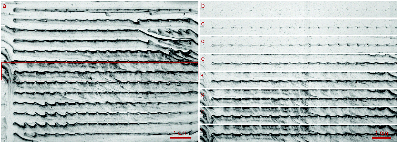 | ||
| Fig. 3 Grown biofilm of K. xylinus in the microfluidic cell growth chamber (see Fig. 2) at a flow rate of 1.0 mm s−1 running from left to right. (a) Due to the panoramic viewing window of the optical setup, the biofilm growth around over 230 obstacles could be determined. The inlet channels, whose exits can be seen on the left, regularly allowed an even distribution of the fluid into the growth chamber. (b)–(i) is the cutout highlighted in (a) by a red frame. (b)–(h) Growth at the middle row in time steps of 6 h. Image (h) corresponds to the large image (a) and captures the moment after 36 h of growth when the pressure reached 1 bar and the flow reduces due to the servo loop. Image (i), unchanged from (h), shows the moment 94 h after the flow rate stagnated due to clogging of the setup. | ||
Scanning electron micrographs showed that the BCB was built from several paper-like layers parallel to the flow, which were continuously connected by BC fibers. Between the obstacles and in the flow direction, the BCB appears to be thicker with a higher fraction of bacteria, which are roughly estimated at 0.01–0.1 ml ml−1. At the higher concentrated spots, the thickness of the dried film only reached a few microns. For brevity, these images are shown as the ESI,† Fig. S2 and Fig. S3.
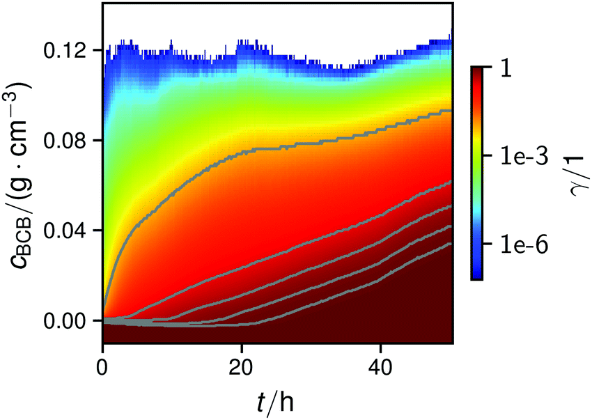 | ||
| Fig. 4 Map of the normalized cumulative histogram γ(cBCB,b,t) at a flow rate of 12.5 mm s−1. The gray plotted lines are isolines of γ = 0.01, 0.25, 0.50, 0.75, and 0.9. They were fitted with a bi-logistic function cBCB(γ,t), eqn (4). | ||
In all conducted experiments, the cBCB of the recorded data did not exceed 0.2 g cm−3 which was below the setup saturation. It should be noted, however that data collection always ended before the second logistic function could reach saturation due to clogging of the setup.
By fitting the histogram data with a bi-logistic function (eqn (4)), parameters from Fig. 5 were obtained. The fits’ uncertainties increase when the data increasingly shows only sections of entire logistic growth curves at high γ.
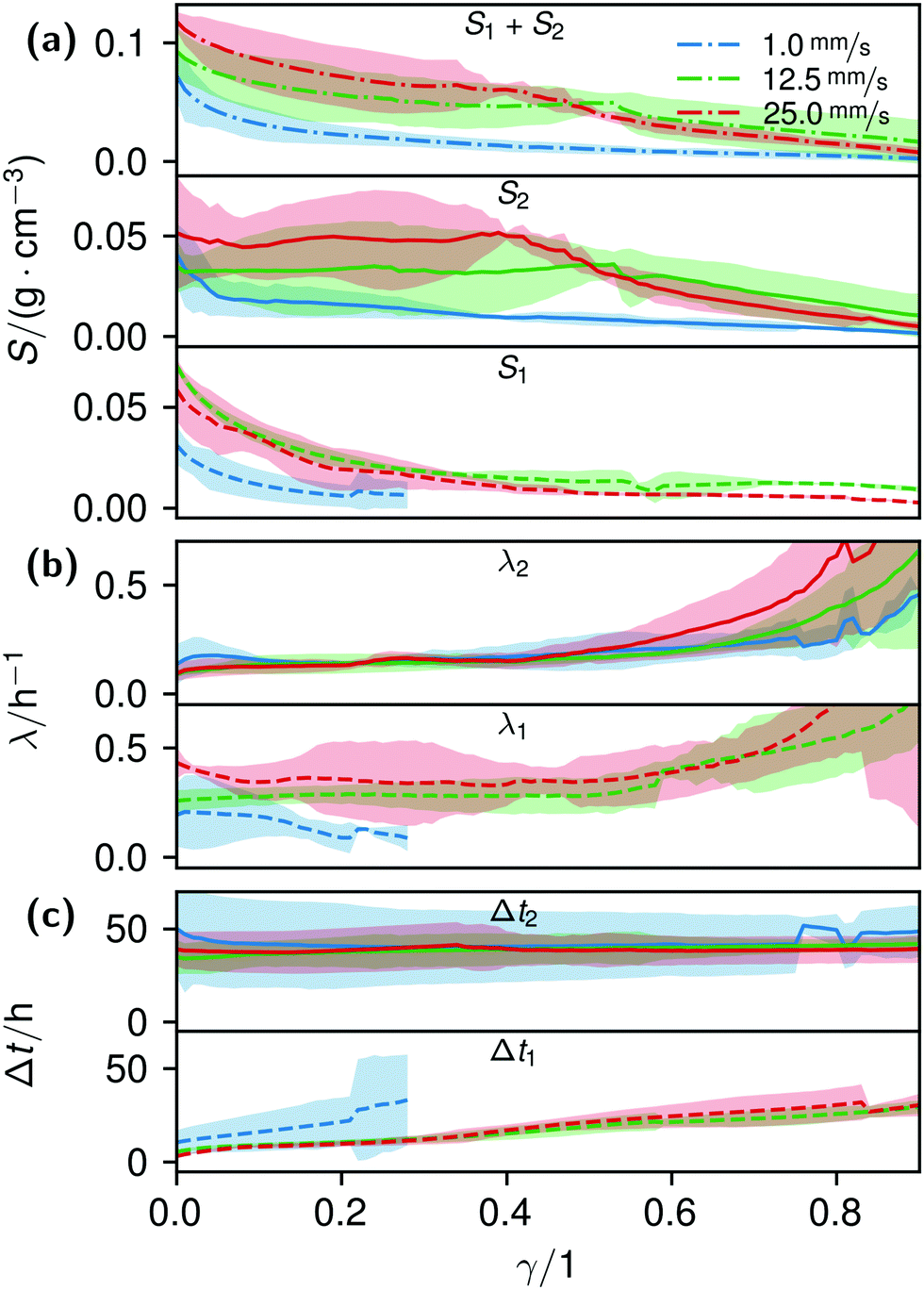 | ||
| Fig. 5 Plots of the histogram parameters (e.g.Fig. 4) from eqn (4). The plots end when the fitted parameter of at least two of the four conducted measurements reached zero, or unrealistic values. Dashed lines (Index 1) are the parameters of the first term, solid lines (Index 2) of the second term of eqn (4). Dash-dotted lines in (a) represent the cumulative values S of the first and second terms. | ||
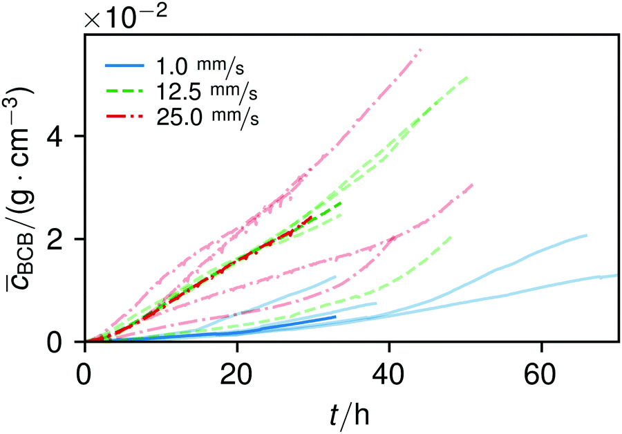 | ||
| Fig. 6 Increase of the average BCB concentration over time, together with the median of the different flow series. To show the variance of the measurements, the data from the single experiments are overlaid in lighter tones. | ||
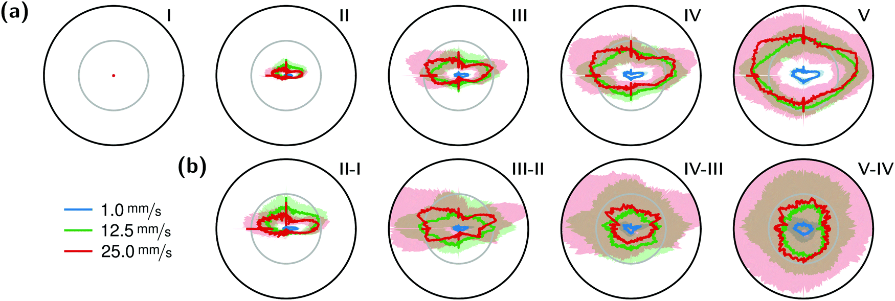 | ||
| Fig. 7 Azimuthal plots of the obstacles’ surroundings with the flow running from left to right in timesteps I–V of 7.5 h, whereby timestep I was 10 minutes after the start. Inner circles in row (a) represent a BCB concentration of 0.02 g cm−3, outer circles 0.04 g cm−3. Row (b) shows the differences between two timesteps from the upper row. Here, the inner circles represent 0.01 g cm−3 and the outer circles 0.02 g cm−3. | ||
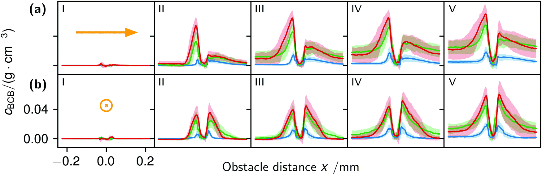 | ||
| Fig. 8 Profile plots parallel (a) and perpendicular (b) to the flow in timesteps I–V of 7.5 h, where timestep I was 10 minutes after the start. The obstacle center is the x-axis center and fluid flow is indicated by the orange arrows. The blue line represents flow at 1.0 mm s−1, the green line at 12.5 mm s−1 and the red line at 25.0 mm s−1. | ||
 | ||
| Fig. 9 Micrographs of cellulose structured at a flow velocity of 1.0 mm s−1. (a) shows a clipping of the last image during the growth experiment near the inlet channels. The orange contour marked the piece of the dried cellulose film (b) which was investigated by polarized light microscopy. Images (c), (f), and (i) shown the sample oriented at −45°, (e), (h), and (k) by +45° and (d), (g), and (j) by 0° in relation to the polarizers. For images (f), (g), and (h), a n λ retardation plate was inserted. | ||
3.2 Flow simulation
The local Reynolds number Re was determined in the CFD simulation for all flow rates. With the results of Remax = 24 in the inlet, Remax = 20 on the chamber and Remax = 3.7 around the obstacles the flow was considered laminar, since all values were below ReKar ∼ 40, at which Karman vortices start to appear after cylindrical obstacles.82Even though the flow was laminar all the time, at higher flow the field at t0 was no longer perfectly distributed in the growth chamber, see Fig. S7 (ESI†). Nevertheless, the wall shear stress τ around parallel obstacles located in the middle of the growth chamber showed a high uniformity at every flow rate (Fig. 11(a)). This also illustrates the spatially resolved flow field, Fig. 10.
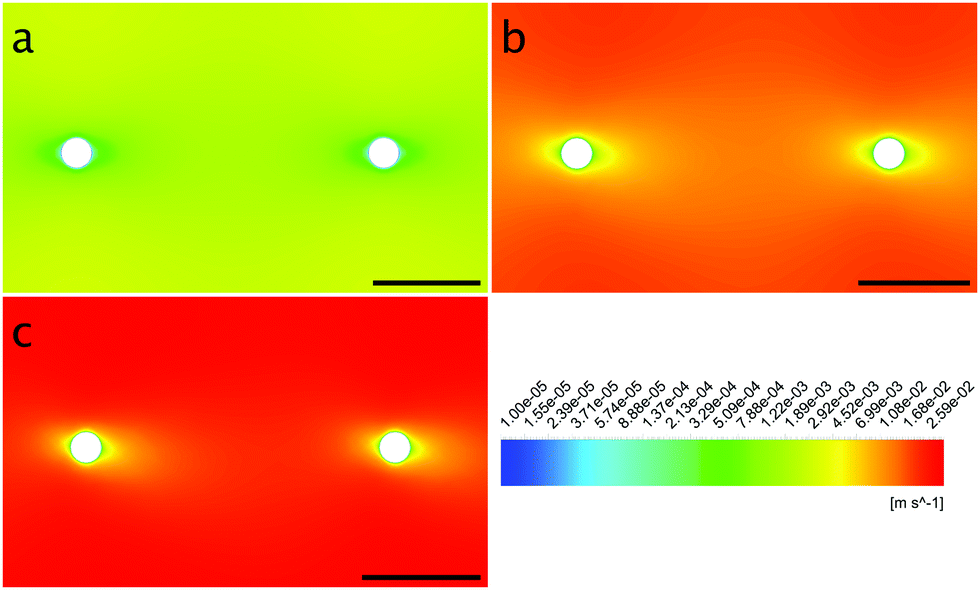 | ||
| Fig. 10 Contour plots of the obstacles’ surroundings at the flow rates 1.0 mm s−1 (a), 12.5 mm s−1 (b) and 25.0 mm s−1 (c) with flow from left to right. | ||
3.3 Mineralisation
Gypsum formation, identified by XRD as CaSO4·2H2O, was observed to be more localised: approximately two minutes after injection, several hundred observable crystals formed. Growth was visibly concentrated on these aggregates which increased their sizes up to half a millimeter. These aggregates consisted of differently sized needles which appeared to have a slightly preferred orientation in the direction of the flow. During drying, the observed number of aggregates and single needle-like crystals smaller than a tenth of a millimeter increased. Small amounts of halite, residual from the mineralisation reagents were observed, but not further considered.
Micrographs of the dried samples of both mineralisation paths showed that the crystals grew on both the BCB surfaces and between the layers, pressing them apart by being embedded in the BC network. An overview of the SEM images can be seen in the Fig. S4 and S5 (ESI†).
| Flow rate/(mm s−1) | Syringe inject rate/(μl s−1) | Syringe volume/ml | Syringe refill rate/(μl s−1) |
|---|---|---|---|
| 1.0 | 0.450 | 1 | 50 |
| 12.5 | 5.625 | 2 | 75 |
| 25.0 | 11.25 | 10 | 100 |
| Mineral | Flow rate/(mm s−1) | # | (hkl) | L/nm | w ⊥/1 | w ‖/1 |
|---|---|---|---|---|---|---|
| Calcite | 1.0 | 1 | (100) | 102 ± 3 | 0.28 ± 0.01 | 0.36 ± 0.01 |
| (001) | 99 ± 4 | 0.44 ± 0.02 | 0.29 ± 0.01 | |||
| 12.5 | 2 | (100) | 104 ± 5 | 0.33 ± 0.01 | 0.38 ± 0.04 | |
| (001) | 103 ± 7 | 0.35 ± 0.02 | 0.24 ± 0.04 | |||
| 25.0 | 3 | (100) | 54 ± 1 | 0.33 ± 0.01 | 0.33 ± 0.01 | |
| (001) | 50 ± 1 | 0.33 ± 0.01 | 0.33 ± 0.01 | |||
| Vaterite | 12.5 | 1 | (100) | 28 ± 0 | 0.30 ± 0.00 | 0.31 ± 0.01 |
| (001) | 27 ± 0 | 0.40 ± 0.01 | 0.37 ± 0.02 | |||
| 25.0 | 3 | (100) | 23 ± 0 | 0.31 ± 0.01 | 0.29 ± 0.01 | |
| (001) | 28 ± 2 | 0.38 ± 0.03 | 0.41 ± 0.03 | |||
| Gypsum | 1.0 | 1 | (100) | 120 ± 7 | 0.04 ± 0.00 | 0.57 ± 0.02 |
| (010) | ≫208 ± 25 | 0.87 ± 0.01 | 0.09 ± 0.00 | |||
| (001) | 123 ± 6 | 0.09 ± 0.00 | 0.33 ± 0.01 | |||
| 12.5 | 2 | (100) | 127 ± 14 | 0.09 ± 0.01 | 0.47 ± 0.04 | |
| (010) | 141 ± 5 | 0.79 ± 0.03 | 0.13 ± 0.01 | |||
| (001) | 122 ± 20 | 0.13 ± 0.01 | 0.40 ± 0.04 | |||
| 25.0 | 1 | (100) | 87 ± 5 | 0.07 ± 0.00 | 0.53 ± 0.02 | |
| (010) | 208 ± 7 | 0.77 ± 0.03 | 0.05 ± 0.00 | |||
| (001) | 116 ± 8 | 0.15 ± 0.01 | 0.41 ± 0.01 |
4 Discussion
4.1 Biofilm growth
To assess the system's productivity, the total volume of the pumped inoculum should be considered. Hence in the observed section, the productivity was (1.8 ± 0.7) × 10−5 g (l h)−1 for 1 mm s−1, (6 ± 2) × 10−6 g (l h)−1 for 12.5 mm s−1 and (3 ± 1) × 10−6 g (l h)−1 for 25.0 mm s−1. These productivities may be low, compared to the values Campano et al. reviewed in their Table 3.83 However, our productivity only represents biomass from the viewing window and not from the whole setup, including the reservoir.
The interesting information from these values, which decrease with higher flow rates is another: they show that the concentration increase rate at higher flow rates is not explicable by a better nutrient or oxygen supply due to the higher agitation. Literature reports confirm that agitated bacteria cultures in general do not necessarily show a better performance than static ones.84,85 A higher biomass production follows from lower velocities, as Krsmanovic et al. reviewed.86 This effect can also be observed in microfluidic systems.45 Considering the production of BCB, Liu et al. found that the cell viability of K. xylinus was clearly increased by agitating. But the data also shows that even low agitation reduced the BCB production. Thus, referring to the BCB yield per cell, the agitation had a strong disadvantageous effect.87 For aligned BCB, Luo et al. found similar results, with an observed biomass reduction from around 38 mg ml−1 to 24 mg ml−1 at flow rates of 30 mm s−1 and 150 mm s−1 (and around 55 mg ml−1 for the static reference).37 The reason for this observation is rather not a genetic mechanosensing, but a prolonged lag-phase due to washout of biofilm substances.44,49
K. xylinus, which can be considered non-motile when floating freely, in principle, is not influenced by flow, except for a rotary type of stroke.51,52 Hence, it ‘goes with the flow’. When the flow hits an obstacle, bacteria adhere to the obstacle. Once adhered, the bacterial BC then facilitates the attachment of further bacteria, leading to their rapid accumulation. The calculated shear stress at the obstacles, Fig. 11(a), supports this idea: with a maximum wall shear stress around 2 Pa for 25.0 mm s−1 perpendicular to the flow direction and a ten times lower minimum at the flow facing direction, we assume that the bacteria withstand the shear force at the flow-facing side. Although we could not find data about the specific adhesion force of K. xylinus to PDMS, it is likely that the critical shear stress, at which attachment and detachment are in balance, is not smaller by orders of magnitudes to P. aeruginosa with 1.1 ± 0.2 Pa, due to their similar shapes and sizes.88 The work of Chaen et al. supports this by demonstrating BCB structuring, formed at an estimated 1 Pa with G. hansenii. In our experiments, it can be assumed that the adhesion is even higher: K. xylinus seems to be more difficult to wash off polar surfaces such as PDMS due to microbial cellulose hydrogen bond attachment.89,90 And additionally, if K. xylinus already extruded fibers, we assume that they further enhance adhesion, making it more difficult to detach.
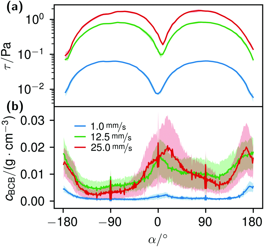 | ||
| Fig. 11 Image (a) shows the calculated wall shear stress around nine parallel obstacles located in the middle of the microfluidic cell at different flow rates. In image (b) the azimuthal concentration cBCB(α) around the obstacles, 15 h after the start of the experiments, is pictured. The flow direction was from 0° to ±180°. | ||
The correlation of the minima and maxima in Fig. 11(a) and (b) indicates that K. xylinus started to form its biofilm with its origin in the areas that were protected from shear forces.85 Hence K. xylinus initially attached to the obstacles’ flow-facing sides, from where it excreted BC, whereby the amount of initial bacteria depended on the flow speed, see sketch Fig. 12, left hand side. Extruded BC then elongated with the flow, embracing the obstacles (Fig. 8(b) (II)) and forming an obstacle-to-obstacle network in the direction of the flow, Fig. 3(b)–(e) and sketch Fig. 12 center image. While for higher flow rates, the median BCB concentration is equal in front of and behind the obstacles (Fig. 7(a)), the spatial distribution has a maximum on the flow-facing side as already illustrated for all flow rates, Fig. 8(a). After the BCB streamers connected after about 10 h, this maximum value does not increase further. Rather, the obstacle-to-obstacle concentration rose, building a highly concentrated network in the direction of the flow, with an increasingly harmonised concentration distribution. All tested flow rates resulted in a distinct obstacle-to-obstacle network. At higher flow, the network was more highly concentrated. This concentration rise can be attributed to a better nutrient supply of the consisting network due to the higher dynamic pressure.
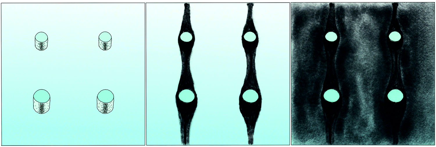 | ||
| Fig. 12 Sketch of the BCB network formation around the PDMS obstacles with the initial bacteria accumulation (left), the first growth phase (middle) and the second growth phase (right). In this sketch, the flow comes from below. | ||
The initial bilateral flow-dependent concentration distributions became weaker with time, as Fig. 7(b) indicates. It changed from being aligned with the flow, to more uniform with and lateral to the flow. The lateral spreading of the BCB can also be observed with its spatial concentration profile in Fig. 8(b). Looking at the single strands, the spreading initially occurs unilaterally and becomes uniform after the strands connected. Fig. 8(b) indicates that when facing the flow, statistically the concentration distribution is slightly shifted to the right. But sometimes, it also occurred left-sided, as it can be seen with the spreading of the BCB in Fig. 3(e)–(g). We speculate that with time, the biofilm also grew in the microfluidic inlet. This caused minimal pressure differences between the grown strands due to different inlet flows. Under perfect initial conditions, the resulting cross flow in principle occurs randomly. But in CFD simulations, the used microfluidic cell already shows a very slight initial cross flow at 12.5 mm s−1 and 25 mm s−1 due to a short inlet channel (Fig. S7, ESI†). It is likely that the observed slight right-handed concentration distribution (Fig. 8(b)) can be contributed to a unilateral biofilm growth in the microfluidic inlet, caused by the initial cross flow. However, since the network concentration equalized with time, this probably had no effect on the final network. Its total concentration distribution becomes more and more uniform and a connected network with higher concentrated regions along the obstacles forms, see sketch Fig. 12, right image.
The angular changes of the total concentration from directional to uniform were visible after a similar growth duration at all tested flow rates with a minimal delay at 1 mm s−1. This becomes visible in Fig. 7(b) IV–III and V–IV and is called the second growth phase in the following, being distinguishable from the first logistic growth phase, Fig. 4. In summary, the growth can be described in two sequential processes: first, the interconnection of the obstacles in the direction of the flow and second, their connection with a general increase of the concentration over the whole biofilm.
The formation of the flow-aligned obstacle-to-obstacle network in the first phase can also be observed in the statistic growth data, as dashed lines in Fig. 5. Since the main concentration is located in the direction of the flow between the obstacles (Fig. 3) and the area of these interspaces equals γ ≈ 0.1, it further can be assumed that the region of the first growth phase below γ = 0.2 in Fig. 5 mainly represents the obstacle-to-obstacle growth. That the relevant values of S1 are mostly in this region fits this assumption. On the basis of the fitted parameters (Fig. 5), the forming of this network becomes traceable: a higher flow rate enhanced the growth constant, the final concentration and shortens the time-point of the inflection. We assume that the former change is due to an ongoing and flow dependent catching of floating bacteria similar to the “fishing-line” observation of Marty et al.91 The change of the latter two started to saturate with a higher flow. On the one hand, in contrast to the second growth phase, nutrients could reach easily the inner of the relatively small strands, while a higher dynamic pressure did not enhance the final concentration by the increased fluent exchange. On the other hand, the inflection time-point stops decreasing. It appears that the lag-phase became the speed-determining step, indicating that influences such as the nutrient resorption of the bacteria and other influences dominated.
The overall increase in concentration at the flow rates 12.5 mm s−1 and 25 mm s−1 in both phases was quite similar in their main grow directions (first phase with the flow; second phase uniformly) and mostly in a range between 0.005 and 0.01 g cm−3 in 7.5 h, see Fig. 7(b). At 1.0 mm s−1 it was around 0.001 g cm−3 in the same time-step. Interestingly, the growth constant of the second growth phase is widely the same for all flow rates, Fig. 5. Different from the “fishing-line” effect in the first phase, in the second growth phase the catching of bacteria seemed no longer to be the dominant mechanism. Rather, an equilibrium was reached at every flow rate, resulting in a growth constant which stayed stable and can be seen as the real growth constant for biofilm with the given culturing parameters. Because on the one hand, by a higher shear stress, more bacteria were embedded in the existing biofilm. On the other hand, there were more high-shear regions, where bacteria and biofilm substances could no longer adhere or become detached. We assume that these high-shear regions arose from a smaller available volume, due to the increasing filling of the microfluidic cell. This is different from the observation by Drescher et al., who consistently saw a more rapid clogging with higher flow rates.45 By contrast to the present work, their setup was pressure-, and not flow-controlled, resulting in a defined maximum flow rate and therefore in a maximum shear stress the biofilms have to endure.
The average BCB concentration increase is nearly the same for 12.5 mm s−1 and 25 mm s−1, Fig. 6. Since a higher flow rate does increase the total concentration over a broad range as in Fig. 5(a), the final average BCB concentrations will differ: Fig. 6 only shows the increase until the setup clogged. The end of this BCB gel redensification was only observable for two of the 1 mm s−1 flow rate experiments after approximately 60–70 h. Since the S2 values in Fig. 5 are extrapolated by obtaining the best fit, it is to be expected that all saturate. The appearing linear increase in Fig. 6 thus was the superposition of both growth phases. In the end, the saturated of 25 mm s−1 then will be higher than that of 12.5 mm s−1. Moreover, the time-point of the saturations can be estimated. Since Δt2 is very similar for all flow rates, and in the region of approximately 40 h, the observed 60–70 h are likely for all flow rates.
The median of the second phases’ inflection points Δt2 and growth constants λ2 changed only insignificantly. It shows, as already stated, that the growth in the second phase was mainly independent of effects like an increased and continuous aggregation of bacteria. It should be noted that due to the increasingly shorter isolines at higher γ, in particular the uncertainty of λ strongly rose, making its interpretation difficult.
Our experiments showed rheotactically aligned BC already at the lowest flow rate of 1 mm s−1, Fig. 9. In images (c)–(k), the birefringence of the long optical axis in the direction of the (001) planes of the highly crystalline bacterial cellulose can be seen. Since the birefringence is strongest visible at ±45° between the flow direction and the crossed microscope polarizers, the fibers which are elongated along the (001) planes were aligned in the direction of the flow. The fact that also higher concentrated regions are outside of the highly concentrated obstacle-to-obstacle strands shows that the majority of the bacterial cellulose was flow-aligned. On closer inspection, the crystalline birefringent regions of the aligned fibers can even be seen in Fig. 9(i), (k) with an approximated mean length of about 10 μm.
Besides the alignment, Chae et al. found, in their flow-driven alignment experiment with the BCB producing G. hansenii, an additional structural characteristic: in contrast to other alignment methods like BC stretching, the BC chains showed parallel packing. This results in macroscopic net dipoles via the alignment from the fibers’ reducing end to their non-reducing end.38 We assume it is possible that the current flow driven alignment approach results in the same packing and that the hierarchical structure features persist even more distinct from the molecular to the macroscopic level by rheotactic structuring compared to other structuring approaches.
4.2 Mineralisation
To obtain a composite material with structured BCB as the substrate, we performed two quasi in situ mineralisations. In the gypsum mineralisation, flower-like gypsum aggregates occurred. Nissinen et al. and Nindiyasari et al.76,94 demonstrated gypsum/cellulose composites with mineralisation from hemihydrate or supersaturated CaCl2–Na2SO4 solutions. The reason for the more uniform crystal distribution and size by Nissinen et al. can be seen in the used cellulose substrate. While Nissinen et al. used a cast cellulosic film, bacterial cellulose consists of ribbon-shaped cellulosic nanofibers with a width of 40–60 nm.25 Cellulose in general can be seen as supportive for gypsum precipitation,94 but the anhydride formed from the supersaturated solution requires water for the hydration steps over bassanite to the final CaSO4·2H2O.95 Water-soaked cellulose can supply an anhydrid nuclei. If the water release decreases, due to a decreasing size of the fibers, the formation of nuclei becomes more unlikely,94 resulting in a degraded and more heterogeneous crystal distribution.To determine whether the anisotropic structure of the substrate affects the orientation of the crystals, we performed two different XRD measurements: measurements with Bragg–Brentano geometry and applied spin, to discriminate texture within or out of the sample plane (w⊥). With measurements in transmission mode, textures along the sample plane in the direction of the flow are determinable (w‖). Gypsum refined XRD data show that L and w⊥ in the direction of the (010) planes are increased against (100) and (001). The (001) planes show the same effect against the (100) planes to a lesser extent, Table 2. Thus the data indicate the texture in two directions: first, the (010) plane of the gypsum crystals, laid parallel to the BC film. This can also be seen in Fig. S5(b)–(d), ESI† where the acerous morphology has a distinct and visible tabular fraction largely facing the observer. We assume that this favored orientation normal to the BCB surface is due to the strong BCB shrinkage, since XRD measurements are obtained after drying. The gypsum crystals were probably twisted by the shrinking in a way that the biggest surface ((010) plane) finally lay between the BC layers, reducing the fibers’ tensions. A slight decrease of this anisotropy with a higher flow rate and thus a higher concentration is explainable by better embedding, reducing the twisting of the crystals. Second, since w‖ of the (100) plane is slightly more distinctive than the (001) plane, slight orientation of the crystals in the direction of the flow is indicated. This orientation is probably caused by heterogeneous nucleation. Some of these crystals then formed large aggregates, which overall showed a slight statistic orientation with the flow, Fig. S5(a), (ESI†). The observed aggregates do not correspond to the determined L values. Since the XRD data represent the whole samples and SEM images are limited to the samples’ surfaces, further evaluation of the interlayer BC structure, which is out of the scope of this work, might resolve the missing correspondence.
The stable ACC suspension was well distributed over the samples, resulting in a good final distribution of CaCO3 with small crystallites embedded in the BCB. Since the directional w does not differ significantly from 0.33, the growth of the obtained CaCO3 phases calcite and vaterite seemed to be isotropic and not affected by the aligned BCB substrate, Table 2. However, the mean crystallite size L of calcite was probably influenced, reducing to half at a flow rate of 25 mm s−1. Due to the lack of repeating measurements for the lower flow rates, this value has some scope for interpretation. But, an influence on L caused by the higher BCB concentration in areas γ < 0.5 is quite possible, since with a larger surface, more heterogeneous nucleation can take place.
We processed a one precursor mineralisation of the BCB samples, immediately after growth in the same setting. This quasi in situ mineralisation route, based on liquid impregnation,72 provides – besides its simplicity – advantages by comparison to other in situ or in vitro routes. Regarding the former, the growth process and thus BC properties such as crystallinity are not affected by mineralisation ingredients and can be conducted at optimal process parameters.59 The latter on the other hand brings along some difficulties by transferring fragile samples into a new vessel where mineralisation can be performed, e.g. by a diffusion based68 or time-consuming gas diffusion based mineralisation.68,96,97 The one-precursor method further was beneficial, since in our setup already minimal rinsing between the reagents prohibited the precipitation and a double diffusion method applied by Grassmann et al.98 was rather inapplicable.
In conclusion, the slight effect of the anisotropic substrate on gypsum crystallisation seems promising for the production of a phase overlapping hierarchical engineering material. Even though gypsum had some limitations, other acerous minerals such as montmorillonite could overcome the insufficient distribution. However, due to its good distribution and embedment, the CaCO3 route seems promising to create a biomimetic organic/inorganic composite. An interesting work was conducted by Yu et al. where a BC composite with tunable toughness was produced.99 It is quite imaginable to apply the presented process with pre-aligned BCB as a substrate in a quasi in situ route. Indeed, fabrication steps like purification by boiling with sodium hydroxide, or blending of the BCB must be adapted. But even if bacteria remain after adaption in the composite similar to our experiments, they can induce interesting properties such as improved absorption capacity or higher maximum tensile/compressive strength.100
4.3 Experimental setup
In principle, three types of biofilm reactors are suited for the targeted rheotactical cultivation of biofilm streamers.101 Rotational reactors, where either the inoculum or the sample is in rotation to produce a flow,36,37 or loop type reactor, where the reactor is fixed and constantly flushed by medium or inoculum. While the former two are mostly used to produce biofilms in large quantities, the latter method is suitable to evaluate biofilms during growth.15,44–46 Besides a better possibility to maintain axenic conditions, the loop type setup enables the use of flow- or pressure driven material synthesis. Since in open or rotational reactors, the inoculum primarily flows on top of the grown BCB, tracing increases in concentration to flow rates, as in this work, is not feasible.The main limitation of the loop setup is the limited space of the reactor (in this work the microfluidic cell). In our experiments, the saturation occurred due to this limitation. While in other reactors, it can be expected that different growth parameters will be obtained, since especially the way of nutrient supply differs by the higher degree of freedom of the medium/inoculum flow, an eventual saturation is inevitable. And, if the structuring element where the BCB grows is similar to the obstacle pattern used in this work, a two phase growth will probably also arise. Hence, for obstacle-induced growth, where a defined microbial streamer shall form a cohesive streamer network, our results give an appropriate basis that can be adapted to produce structured material with loop type reactors, but also with rotational reactors.36,37 To summarise, with our loop type reactor with a panorama view observation setup, we were able to observe the formation of the BCB network and spatial streamers simultaneously. To our best knowledge, investigation about the formation of larger bacterial streamer networks, in particular BCB streamer networks are not available. Thus, the flow-influenced formation of two hierarchical levels could be observed directly, knowing that also the subjacent levels like the direction of the cellulose fibers and ribbons are aligned by the flow, as apparent in Fig. 9.
Our method is suitable to measure the BCB concentration profile over the grown network via the Lambert–Beer equation in a dynamic range of 1![[thin space (1/6-em)]](https://www.rsc.org/images/entities/char_2009.gif) :932. Even after several days of growth, the optical examination did not reach its saturation. Besides the attenuation of the light by BCB, a slight (focused) shadowgraph effect was visible at the thin edges between BCB and the surrounding inoculum (e.g. visible in Fig. 3(f) at the spreading BCB edge). This effect was caused by different refractive indexes of the inoculum and the BCB and the resulting refractive gradient.102 On the one hand, this effect resulted in a minimal and spatial finite overestimation of low measured BCB concentrations, but on the other hand the advantage is that the boundary layers become more visible. By including negative attenuation, our evaluation of the growth data was not affected by this focused shadowgraphy effect. Furthermore, at high refractive gradient edges caused by a higher BCB concentration, the effect largely disappeared, since the light attenuation of the BCB reduced the amount of deflected light.
:932. Even after several days of growth, the optical examination did not reach its saturation. Besides the attenuation of the light by BCB, a slight (focused) shadowgraph effect was visible at the thin edges between BCB and the surrounding inoculum (e.g. visible in Fig. 3(f) at the spreading BCB edge). This effect was caused by different refractive indexes of the inoculum and the BCB and the resulting refractive gradient.102 On the one hand, this effect resulted in a minimal and spatial finite overestimation of low measured BCB concentrations, but on the other hand the advantage is that the boundary layers become more visible. By including negative attenuation, our evaluation of the growth data was not affected by this focused shadowgraphy effect. Furthermore, at high refractive gradient edges caused by a higher BCB concentration, the effect largely disappeared, since the light attenuation of the BCB reduced the amount of deflected light.
Since the attenuation coefficient of BCB is relatively high compared to other EPS, the manner observation was sufficient. But, when growing biofilm streamers consisting of other bacteria and EPS, the sensitivity of the EPS detection and thus the determination of the concentration could become an issue, when the attenuation coefficient is lower. Here, the focused shadowgraphy or even better the schlieren techniques could play a major role in the sensitivity enhancement. Simply inserting a knife edge in the optional optical filter ((9) in Fig. 1) with a cutoff of 80% would intensify the refractive gradient edge by a factor of 5. Changing the lens to f = 500 mm would enhance the factor with the same cutoff to 25.103
5 Outlook
We investigated the rheotactically formation of a bacterial cellulose network consisting of several single bacterial streamers. The formation could be separated into two logistic growth phases. The first was the strain formation between the streamers in the direction of the flow. In the second phase, the grown strains connected, building a hierarchically structured BCB network with flow-aligned BC fibers. The first phase was dependent on the flow rate, since a higher flow provided the streamers with more bacteria. In the second phase, a higher flow with its higher dynamic pressure resulted in a higher final BCB concentration. These findings may form the basis for an upscaled material production of anisotropic cellulose substrates. With the flow rate and design of the flow reactor the concentration and distribution of the aligned BCB in the strands and in the whole material can be adjusted. A BCB-material interwoven with tailored BCB-strands can then be adapted to meet specific mechanical requirements.We also conducted a quasi in situ mineralisation route to trace crystal growth in the hierarchically organised BCB. With ACC and a supersaturated CaSO4 solution, mineral deposition was obtained. CaCO3 thereby showed a more uniform distribution than gypsum. However, with the deposition of the needle shaped gypsum crystals, the anisotropic substrate features could be continued from the organic to the inorganic phase. It is quite conceivable that other minerals e.g. from the group of montmorillonite, or a biomineralisation parth are sufficient for anisotropic hierarchical structured composites. These results illustrate that an evenly distributed mineral phase is attainable. This, in turn, can be utilised to tune the mechanical properties of bio-mimetic hierarchically structured BCB-mineral composite materials. Future applications of the obtained materials thereby could be manifold: in addition to obtaining tough materials, tailor-made surfaces for use as catalysis carriers, for defined adsorption tasks, or as a stationary phase in separating columns are also conceivable.
Author contributions
Moritz Klotz: data curation, formal analysis, investigation, methodology, validation, visualization, writing – original draft. Dardan Bajrami: software (CFD), formal analysis (CFD). Daniel Van Opdenbosch: conceptualization, funding acquisition, project administration, supervision, writing – review & editing.Conflicts of interest
There are no conflicts to declare.Acknowledgements
We thank the German Science Foundation (DFG) for funding our research via grant VA 1349/5.References
- P. Fratzl and R. Weinkamer, Nature's hierarchical materials, Prog. Mater. Sci., 2007, 52(8), 1263–1334 CrossRef CAS.
- C. Mattheck and I. Tesari, The mechanical self-optimisation of trees, WIT Trans. Ecol. Environ., 2004, 73, 10 Search PubMed.
- A. Öchsner, W. Ahmed, J. Fish and T. Belytschko, Biomechanics of Hard Tissues, Wiley Online Library, 2011 Search PubMed.
- G. E. Fantner, E. Oroudjev, G. Schitter, L. S. Golde, P. Thurner, M. M. Finch, P. Turner, T. Gutsmann, D. E. Morse and H. Hansma, et al., Sacrificial bonds and hidden length: Unraveling molecular mesostructures in tough materials, Biophys. J., 2006, 90(4), 1411–1418 CrossRef CAS PubMed.
- P. Greil, T. Lifka and A. Kaindl, Biomorphic cellular silicon carbide ceramics from wood: I. processing and microstructure, J. Eur. Ceram. Soc., 1998, 18(14), 1961–1973 CrossRef CAS.
- D. Van Opdenbosch, M. Thielen, R. Seidel, G. Fritz-Popovski, T. Fey, O. Paris, T. Speck and C. Zollfrank, The pomelo peel and derived nanoscale-precision gradient silica foams, Bioinspired, Biomimetic Nanobiomater., 2012, 1(2), 117–122 CrossRef CAS.
- G. Fritz-Popovski, R. Morak, T. Schöberl, D. Van Opdenbosch, C. Zollfrank and O. Paris, Pore characteristics and mechanical properties of silica templated by wood, Bioinspired, Biomimetic Nanobiomater., 2014, 3(3), 160–168 CrossRef.
- D. Van Opdenbosch, G. Fritz-Popovski, W. Wagermaier, O. Paris and C. Zollfrank, Moisture-driven ceramic bilayer actuators from a biotemplating approach, Adv. Mater., 2016, 28(26), 5235–5240 CrossRef CAS PubMed.
- H. Imai, Self-organized formation of hierarchical structures, in Biomineralization I, Springer, 2006, pp. 43–72 Search PubMed.
- S. Deuerling, S. Kugler, M. Klotz, C. Zollfrank and D. Van Opdenbosch, A perspective on bio-mediated material structuring, Adv. Mater., 2018, 30(19), 1703656 CrossRef PubMed.
- D.-P. Häder, Wie orientieren sich Cyanobakterien im Licht, Biol. Unserer Zeit, 1984, 14(3), 78–83 CrossRef.
- J. Arlt, V. A. Martinez, A. Dawson, T. Pilizota and W. C. Poon, Painting with light-powered bacteria, Nat. Commun., 2018, 9, 1–7 CrossRef CAS PubMed.
- M. Klotz, S. Deuerling, S. Kugler, C. Zollfrank and D. Van, Opdenbosch, light-diffractive patterning of porphyridium purpureum, Photochem. Photobiol. Sci., 2020, 22–34 Search PubMed.
- X.-X. Wang, L. Xie and R. Wang, Biological fabrication of nacreous coating on titanium dental implant, Biomaterials, 2005, 26(31), 6229–6232 CrossRef CAS PubMed.
- R. Rusconi, S. Lecuyer, N. Autrusson, L. Guglielmini and H. A. Stone, Secondary flow as a mechanism for the formation of biofilm streamers, Biophys. J., 2011, 100(6), 1392–1399 CrossRef CAS PubMed.
- Y. Uraki, J. Nemoto, H. Otsuka, Y. Tamai, J. Sugiyama, T. Kishimoto, M. Ubukata, H. Yabu, M. Tanaka and M. Shimomura, Honeycomb-like architecture produced by living bacteria, Gluconacetobacter xylinus, Carbohydr. Polym., 2007, 69(1), 1–6 CrossRef CAS.
- N. Oxman, J. Laucks, M. Kayser, J. Duro-Royo and C. Gonzales-Uribe, Silk pavilion: a case study in fiber-based digital fabrication, in FABRICATE Conference Proceedings, ta Verla, 2014, 248-255.
- J. Loehr, D. Pfeiffer, D. Schüler and T. M. Fischer, Magnetic guidance of the magnetotactic bacterium magnetospirillum gryphiswaldense, Soft Matter, 2016, 12(15), 3631–3635 RSC.
- C. Pierce, E. Mumper, E. Brown, J. Brangham, B. Lower, S. Lower, F. Yang and R. Sooryakumar, Tuning bacterial hydrodynamics with magnetic fields, Phys. Rev. E, 2017, 95(6), 062612 CrossRef CAS PubMed.
- E. Bonabeau, G. Theraulaz, J.-L. Deneubourg, S. Aron and S. Camazine, Selforganization in social insects, Trends Ecol. Evol., 1997, 12(5), 188–193 CrossRef CAS PubMed.
- Z. Lewandowski and H. Beyenal, Fundamentals of Biofilm Research, CRC press, 2013 Search PubMed.
- I. Dogsa, M. Kriechbaum, D. Stopar and P. Laggner, Structure of bacterial extracellular polymeric substances at different pH values as determined by SAXS, Biophys. J., 2005, 89(4), 2711–2720 CrossRef CAS PubMed.
- T. Coviello, W. Burchard, E. Geissler and D. Maier, Static and dynamic light scattering by a thermoreversible gel from Rhizobium leguminosarum 8002 exopolysaccharide, Macromolecules, 1997, 30(7), 2008–2015 CrossRef CAS.
- S. Koizumi, Y. Tomita, T. Kondo and T. Hashimoto, What factors determine hierarchical structure of microbial cellulose -interplay among physics, chemistry and biology, in Macromolecular Symposia, Wiley Online Library, 2009, vol. 279, 1, pp. 110–118 Search PubMed.
- P. Zugenmaier, Crystalline cellulose and derivatives: characterization and structures, Berlin Heidelberg, Springer, 2008 Search PubMed.
- T. Kondo and W. Kasai, Autonomous bottom-up fabrication of three-dimensional nano/microcellulose honeycomb structures, directed by bacterial nanobuilder, J. Biosci. Bioeng., 2014, 118(4), 482–487 CrossRef CAS PubMed.
- T. Kondo, M. Nojiri, Y. Hishikawa, E. Togawa, D. Romanovicz and R. M. Brown, Biodirected epitaxial nanodeposition of polymers on oriented macromolecular templates, Proc. Natl. Acad. Sci. U. S. A., 2002, 99(22), 14008–14013 CrossRef CAS PubMed.
- A. Nagashima, T. Tsuji and T. Kondo, A uniaxially oriented nanofibrous cellulose scaffold from pellicles produced by Gluconacetobacter xylinus in dissolved oxygen culture, Carbohydr. Polym., 2016, 135, 215–224 CrossRef CAS PubMed.
- A. Putra, A. Kakugo, H. Furukawa, J. P. Gong, Y. Osada, T. Uemura and M. Yamamoto, Production of bacterial cellulose with well oriented fibril on PDMS substrate, Polym. J., 2008, 40(2), 137–142 CrossRef CAS.
- S. Zang, Z. Sun, K. Liu, G. Wang, R. Zhang, B. Liu and G. Yang, Ordered manufactured bacterial cellulose as biomaterial of tissue engineering, Mater. Lett., 2014, 128, 314–318 CrossRef CAS.
- J. Yang, L. Wang, W. Zhang, Z. Sun, Y. Li, M. Yang, D. Zeng, B. Peng, W. Zheng and X. Jiang, et al., Reverse reconstruction and bioprinting of bacterial cellulose-based functional total intervertebral disc for therapeutic implantation, Small, 2018, 14(7), 1702582 CrossRef PubMed.
- A. Putra, A. Kakugo, H. Furukawa, J. P. Gong and Y. Osada, Tubular bacterial cellulose gel with oriented fibrils on the curved surface, Polymer, 2008, 49(7), 1885–1891 CrossRef CAS.
- A. Putra, A. Kakugo, H. Furukawa and J. P. Gong, Orientated bacterial cellulose culture controlled by liquid substrate of silicone oil with different viscosity and thickness, Polym. J., 2009, 41(9), 764–770 CrossRef CAS.
- M. B. Sano, A. D. Rojas, P. Gatenholm and R. V. Davalos, Electromagnetically controlled biological assembly of aligned bacterial cellulose nanofibers, Ann. Biomed. Eng., 2010, 38(8), 2475–2484 CrossRef PubMed.
- M. Liu, C. Zhong, X. Zheng, L. Ye, T. Wan and S. R. Jia, Oriented bacterial celluloseglass fiber nanocomposites with enhanced tensile strength through electric field, Fibers Polym., 2017, 18(7), 1408–1412 CrossRef CAS.
- Y. Wan, D. Hu, G. Xiong, D. Li, R. Guo and H. Luo, Directional fluid induced self-assembly of oriented bacterial cellulose nanofibers for potential biomimetic tissue engineering scaffolds, Mater. Chem. Phys., 2015, 149, 7–11 CrossRef.
- H. Luo, W. Li, Z. Yang, H. Ao, G. Xiong, Y. Zhu, J. Tu and Y. Wan, Preparation of oriented bacterial cellulose nanofibers by flowing medium-assisted biosynthesis and influence of flowing velocity, J. Polym. Eng., 2018, 38(3), 299–305 CrossRef CAS.
- I. Chae, S. M. Bokhari, X. Chen, R. Zu, K. Liu, A. Borhan, V. Gopalan, J. M. Catchmark and S. H. Kim, Shear-induced unidirectional deposition of bacterial cellulose microfibrils using rising bubble stream cultivation, Carbohydr. Polym., 2021, 255, 117328 CrossRef CAS PubMed.
- S. Das and A. Kumar, Formation and post-formation dynamics of bacterial biofilm streamers as highly viscous liquid jets, Sci. Rep., 2014, 4(1), 1–6 CAS.
- A. Persat, C. D. Nadell, M. K. Kim, F. Ingremeau, A. Siryaporn, K. Drescher, N. S. Wingreen, B. L. Bassler, Z. Gitai and H. A. Stone, The mechanical world of bacteria, Cell, 2015, 161(5), 988–997 CrossRef CAS PubMed.
- A. Karimi, D. Karig, A. Kumar and A. Ardekani, Interplay of physical mechanisms and biofilm processes: Review of microfluidic methods, Lab Chip, 2015, 15(1), 23–42 RSC.
- Y. Yawata, J. Nguyen, R. Stocker and R. Rusconi, Microfluidic studies of biofilm formation in dynamic environments, J. Bacteriol., 2016, 198(19), 2589–2595 CrossRef CAS PubMed.
- M. G. Mazza, The physics of biofilms: An introduction, J. Phys. D: Appl. Phys., 2016, 49(20), 203001 CrossRef.
- P. Thomen, J. Robert, A. Monmeyran, A.-F. Bitbol, C. Douarche and N. Henry, Bacterial biofilm under flow: First a physical struggle to stay, then a matter of breathing, PLoS One, 2017, 12(4), 1–24 CrossRef PubMed.
- K. Drescher, Y. Shen, B. L. Bassler and H. A. Stone, Biofilm streamers cause catastrophic disruption of flow with consequences for environmental and medical systems, Proc. Natl. Acad. Sci. U. S. A., 2013, 110(11), 4345–4350 CrossRef CAS PubMed.
- A. Marty, C. Roques, C. Causserand and P. Bacchin, Formation of bacterial streamers during filtration in microfluidic systems, Biofouling, 2012, 28(6), 551–562 CrossRef PubMed.
- R. Rusconi, S. Lecuyer, L. Guglielmini and H. A. Stone, Laminar flow around corners triggers the formation of biofilm streamers, J. R. Soc., Interface, 2010, 7(50), 1293–1299 CrossRef PubMed.
- D. R. Espeso and A. M.-C. Rodriguez, Modeling and simulation of bacterial biofilms, PhD dissertation, Universidad Carlos III de Madrid, 2013 Search PubMed.
- N. B. Aznaveh, M. Safdar, G. Wolfaardt and J. Greener, Micropatterned biofilm formations by laminar flow-templating, Lab Chip, 2014, 14(15), 2666–2672 RSC.
- P. Stoodley, R. Cargo, C. J. Rupp, S. Wilson and I. Klapper, Biofilm material properties as related to shear-induced deformation and detachment phenomena, J. Ind. Microbiol. Biotechnol., 2002, 29(6), 361–367 CrossRef CAS PubMed.
- M. Marcos, H. Fu, T. Powers and R. Stocker, Bacterial rheotaxis, Bull. Am. Phys. Soc., 2011, 109, 4780–4785 Search PubMed.
- J. D. Wheeler, E. Secchi, R. Rusconi and R. Stocker, Not just going with the flow: The effects of fluid flow on bacteria and plankton, Annu. Rev. Cell Dev. Biol., 2019, 35, 213–237 CrossRef CAS PubMed.
- J. A. Aufrecht, J. D. Fowlkes, A. N. Bible, J. Morrell-Falvey, M. J. Doktycz and S. T. Retterer, Pore-scale hydrodynamics influence the spatial evolution of bacterial biofilms in a microfluidic porous network, PLoS One, 2019, 14(6), e0218316 CrossRef CAS PubMed.
- M. Hassanpourfard, Z. Nikakhtari, R. Ghosh, S. Das, T. Thundat, Y. Liu and A. Kumar, Bacterial floc mediated rapid streamer formation in creeping flows, Sci. Rep., 2015, 5(1), 1–12 CrossRef PubMed.
- M. Hassanpourfard, R. Ghosh, T. Thundat and A. Kumar, Dynamics of bacterial streamers induced clogging in microfluidic devices, Lab Chip, 2016, 16(21), 4091–4096 RSC.
- N. Shah, M. Ul-Islam, W. A. Khattak and J. K. Park, Overview of bacterial cellulose composites: A multipurpose advanced material, Carbohydr. Polym., 2013, 98(2), 1585–1598 CrossRef CAS PubMed.
- W. Liu, H. Du, M. Zhang, K. Liu, H. Liu, H. Xie, X. Zhang and C. Si, Bacterial cellulosebased composite scaffolds for biomedical applications: A review, ACS Sustainable Chem. Eng., 2020, 8(20), 7536–7562 CrossRef CAS.
- Z. Cheng, Z. Ye, A. Natan, Y. Ma, H. Li, Y. Chen, L. Wan, C. Aparicio and H. Zhu, Boneinspired mineralization with highly aligned cellulose nanofibers as template, ACS Appl. Mater. Interfaces, 2019, 11(45), 42486–42495 CrossRef CAS PubMed.
- F. Mohammadkazemi, M. Faria and N. Cordeiro, In situ biosynthesis of bacterial nanocellulose-CaCO3 hybrid bionanocomposite: One-step process, Mater. Sci. Eng., C, 2016, 65, 393–399 CrossRef CAS PubMed.
- G. Serafica, R. Mormino and H. Bungay, Inclusion of solid particles in bacterial cellulose, Appl. Microbiol. Biotechnol., 2002, 58(6), 756–760 CrossRef CAS PubMed.
- S. Yano, H. Maeda, M. Nakajima, T. Hagiwara and T. Sawaguchi, Preparation and mechanical properties of bacterial cellulose nanocomposites loaded with silica nanoparticles, Cellulose, 2008, 15(1), 111–120 CrossRef CAS.
- M. Pommet, J. Juntaro, J. Y. Heng, A. Mantalaris, A. F. Lee, K. Wilson, G. Kalinka, M. S. Shaffer and A. Bismarck, Surface modification of natural fibers using bacteria: Depositing bacterial cellulose onto natural fibers to create hierarchical fiber reinforced nanocomposites, Biomacromolecules, 2008, 9(6), 1643–1651 CrossRef CAS PubMed.
- S. Shi, S. Chen, X. Zhang, W. Shen, X. Li, W. Hu and H. Wang, Biomimetic mineralization synthesis of calcium-deficient carbonate-containing hydroxyapatite in a three-dimensional network of bacterial cellulose, J. Chem. Technol. Biotechnol., 2009, 84(2), 285–290 CrossRef CAS.
- Y. Wan, Y. Huang, C. Yuan, S. Raman, Y. Zhu, H. Jiang, F. He and C. Gao, Biomimetic synthesis of hydroxyapatite/bacterial cellulose nanocomposites for biomedical applications, Mater. Sci. Eng., C, 2007, 27(4), 855–864 CrossRef CAS.
- M. Ul-Islam, T. Khan and J. K. Park, Nanoreinforced bacterial cellulose-montmorillonite composites for biomedical applications, Carbohydr. Polym., 2012, 89(4), 1189–1197 CrossRef CAS PubMed.
- N. Khodamoradi, V. Babaeipour and M. Sirousazar, Bacterial cellulose/montmorillonite bionanocomposites prepared by immersion and in-situ methods: Structural, mechanical, thermal, swelling and dehydration properties, Cellulose, 2019, 26(13), 7847–7861 CrossRef CAS.
- J. Sun and B. Bhushan, Hierarchical structure and mechanical properties of nacre: A review, RSC Adv., 2012, 2(20), 7617–7632 RSC.
- M. W. Rauch, M. Dressler, H. Scheel, D. Van Opdenbosch and C. Zollfrank, Mineralization of calcium carbonates in cellulose gel membranes, Eur. J. Inorg. Chem., 2012,(32), 5192–5198 CrossRef CAS.
- D. Kuo, T. Nishimura, S. Kajiyama and T. Kato, Bioinspired environmentally friendly amorphous CaCO3-based transparent composites comprising cellulose nanofibers, ACS Omega, 2018, 3(10), 12722–12729 CrossRef CAS PubMed.
- D. Gebauer, V. Oliynyk, M. Salajkova, J. Sort, Q. Zhou, L. Bergström and G. Salazar-Alvarez, A transparent hybrid of nanocrystalline cellulose and amorphous calcium carbonate nanoparticles, Nanoscale, 2011, 3(9), 3563–3566 RSC.
- T. Saito, Y. Oaki, T. Nishimura, A. Isogai and T. Kato, Bioinspired stiff and flexible composites of nanocellulose-reinforced amorphous CaCO3, Mater. Horiz., 2014, 1(3), 321–325 RSC.
- M. Stroescu, A. Stoica-Guzun, S. I. Jinga, T. Dobre, I. M. Jipa and L. M. Dobre, Influence of sodium dodecyl sulfate and cetyl trimethylammonium bromide upon calcium carbonate precipitation on bacterial cellulose, Korean J. Chem. Eng., 2012, 29(9), 1216–1223 CrossRef CAS.
- Q. Zhu, J. Wang, J. Sun and Q. Wang, Preparation and characterization of regenerated cellulose biocomposite film filled with calcium carbonate by in situ precipitation, BioResources, 2020, 15(4), 7893 CAS.
- M. Ciobanu, E. Bobu and F. Ciolacu, In situ cellulose fibres loading with calcium carbonate precipitated by different methods, Cellul. Chem. Technol., 2010, 44(9), 379 CAS.
- A. Stoica-Guzun, M. Stroescu, S. Jinga, I. Jipa, T. Dobre and L. Dobre, Ultrasound influence upon calcium carbonate precipitation on bacterial cellulose membranes, Ultrason. Sonochem., 2012, 19(4), 909–915 CrossRef CAS PubMed.
- T. Nissinen, M. Li, N. Brielles and S. Mann, Calcium sulfate hemihydrate-mediated crystallization of gypsum on Ca2+-activated cellulose thin films, CrystEngComm, 2013, 15(19), 3793–3798 RSC.
- M. Iguchi, S. Yamanaka and A. Budhiono, Bacterial cellulose: A masterpiece of nature's arts, J. Mater. Sci., 2000, 35(2), 261–270 CrossRef CAS.
- A. D. Edelstein, M. A. Tsuchida, N. Amodaj, H. Pinkard, R. D. Vale and N. Stuurman, Advanced methods of microscope control using μManager software, J. Biol. Methods, 2014, 1(2), 1–18 Search PubMed.
- J. Bergmann, P. Friedel and R. Kleeberg, BGMN – a new fundamental parameters based Rietveld program for laboratory X-ray sources, its use in quantitative analysis and structure investigations, CPD Newsletter, 1998, 20, 5–8 Search PubMed.
- N. Doebelin and R. Kleeberg, Profex: A graphical user interface for the Rietveld refinement program BGMN, J. Appl. Crystallogr., 2015, 48(5), 1573–1580 CrossRef CAS PubMed.
- M. Järvinen, Texture models in powder diffraction analysis, in Materials Science Forum, Trans Tech Publ, 1998, vol. 278, pp. 184–199 Search PubMed.
- J. H. Lienhard, et al., Synopsis of lift, drag, and vortex frequency data for rigid circular cylinders, Technical Extension Service, Washington State University Pullman, WA, 1966, vol. 300 Search PubMed.
- C. Campano, A. Balea, A. Blanco and C. Negro, Enhancement of the fermentation process and properties of bacterial cellulose: A review, Cellulose, 2016, 23(1), 57–91 CrossRef CAS.
- W. Czaja, D. Romanovicz and R. Malcolm Brown, Structural investigations of microbial cellulose produced in stationary and agitated culture, Cellulose, 2004, 11(3), 403–411 CrossRef CAS.
- P. Singhsa, R. Narain and H. Manuspiya, Physical structure variations of bacterial cellulose produced by different Komagataeibacter xylinus strains and carbon sources in static and agitated conditions, Cellulose, 2018, 25(3), 1571–1581 CrossRef CAS.
- M. Krsmanovic, D. Biswas, H. Ali, A. Kumar, R. Ghosh and A. K. Dickerson, Hydrodynamics and surface properties influence biofilm proliferation, Adv. Colloid Interface Sci., 2020, 102336 Search PubMed.
- M. Liu, C. Zhong, X.-Y. Wu, Y.-Q. Wei, T. Bo, P.-P. Han and S.-R. Jia, Metabolomic profiling coupled with metabolic network reveals differences in Gluconacetobacter xylinus from static and agitated cultures, Biochem. Eng. J., 2015, 101, 85–98 CrossRef CAS.
- M. R. Nejadnik, H. C. Van Der Mei, H. J. Busscher and W. Norde, Determination of the shear force at the balance between bacterial attachment and detachment in weakadherence systems, using a flow displacement chamber, Appl. Environ. Microbiol., 2008, 74(3), 916–919 CrossRef CAS PubMed.
- J. Kuncova-Kallio and P. J. Kallio, PDMS and its suitability for analytical microfluidic devices, in 2006 International Conference of the IEEE Engineering in Medicine and Biology Society. IEEE, 2006, 2486-2489.
- D. J. Gardner, G. S. Oporto, R. Mills and M. A.-S. A. Samir, Adhesion and surface issues in cellulose and nanocellulose, J. Adhes. Sci. Technol., 2008, 22(5-6), 545–567 CrossRef CAS.
- A. Marty, C. Causserand, C. Roques and P. Bacchin, Impact of tortuous flow on bacteria streamer development in microfluidic system during filtration, Biomicrofluidics, 2014, 8(1), 014105 CrossRef CAS PubMed.
- R. Holm and D. Söderberg, Shear influence on fibre orientation, Rheol. Acta, 2007, 46(5), 721–729 CrossRef CAS.
- S. B. Lindström and T. Uesaka, Simulation of semidilute suspensions of non-brownian fibers in shear flow, J. Chem. Phys., 2008, 128(2), 024901 CrossRef PubMed.
- F. Nindiyasari, E. Griesshaber, T. Zimmermann, A. P. Manian, C. Randow, R. Zehbe, L. Fernandez-Diaz, A. Ziegler, C. Fleck and W. W. Schmahl, Characterization and mechanical properties investigation of the cellulose/gypsum composite, J. Compos. Mater., 2016, 50(5), 657–672 CrossRef CAS.
- A. Van Driessche, L. G. Benning, J. Rodriguez-Blanco, M. Ossorio, P. Bots and J. García-Ruiz, The role and implications of bassanite as a stable precursor phase to gypsum precipitation, Science, 2012, 336(6077), 69–72 CrossRef CAS PubMed.
- H. K. Raut, A. F. Schwartzman, R. Das, F. Liu, L. Wang, C. A. Ross and J. G. Fernandez, Tough and strong: Cross-lamella design imparts multifunctionality to biomimetic nacre, ACS Nano, 2020, 14(8), 9771–9779 CrossRef CAS PubMed.
- A.-W. Xu, M. Antonietti, H. Cölfen and Y.-P. Fang, Uniform hexagonal plates of vaterite CaCO3 mesocrystals formed by biomimetic mineralization, Adv. Funct. Mater., 2006, 16(7), 903–908 CrossRef CAS.
- O. Grassmann and P. Löbmann, Morphogenetic control of calcite crystal growth in sulfonic acid based hydrogels, Chem. – Eur. J., 2003, 9(6), 1310–1316 CrossRef CAS PubMed.
- K. Yu, E. M. Spiesz, S. Balasubramanian, D. T. Schmieden, A. S. Meyer and M.-E. Aubin-Tam, Scalable bacterial production of moldable and recyclable biomineralized cellulose with tunable mechanical properties, Cell Rep. Phys. Sci., 2021, 100464 CrossRef CAS.
- Y. Wan, J. Wang, M. Gama, R. Guo, Q. Zhang, P. Zhang, F. Yao and H. Luo, Biofabrication of a novel bacteria/bacterial cellulose composite for improved adsorption capacity, Composites, Part A, 2019, 125, 105560 CrossRef CAS.
- H. Kanematsu and D. M. Barry, Formation and control of biofilm in various environments, Singapore, Springer, 2020 Search PubMed.
- G. S. Settles and E. Covert, Schlieren and shadowgraph techniques: Visualizing phenomena in transport media, Appl. Mech. Rev., 2002, 55(4), B76–B77 CrossRef.
- G. S. Settles, Schlieren and Shadowgraph Techniques, Berlin Heidelberg New York, Springer, 2006 Search PubMed.
Footnote |
| † Electronic supplementary information (ESI) available: See DOI: https://doi.org/10.1039/d2ma00115b |
| This journal is © The Royal Society of Chemistry 2022 |