Hybrid machine-learning-assisted quantification of the compound internal and external uncertainties of graphene: towards inclusive analysis and design

Abstract

Molecular dynamics (MD) simulations have emerged to be a vital tool for the analysis of nanoscale materials like graphene. However, the reliability of the results derived from MD simulations depends on the adopted inter-atomic potential (IP), which is mathematically fitted to the data obtained from first principles approaches or experiments. There exists a significant scope of uncertainty associated with the IP parameters. Such internal uncertainties, together with the effect of stochastic external parameters like temperature and strain rate can trigger an augmented random deviation in the output mechanical responses. With the aim of developing an inclusive analysis and design paradigm, we have systematically quantified the effect of the uncertainties associated with the internal parameters (Tersoff IP parameters) and external parameters (temperature and strain rate) individually, and their compound effect on the mechanical properties of graphene. In establishing the complete probabilistic descriptions of the response quantities corresponding to different levels of source uncertainties, we show that a coupled machine learning-based Monte Carlo simulation approach could lead to significant computational efficiency without compromising the accuracy of the results. The study reveals that, in general, the internal parameters are more sensitive than the external parameters. Among the inter-atomic parameters, λ₁ and λ₂ are found to be the most sensitive, while the temperature is found to be more sensitive than the strain rate among the external parameters. The cohesive energy is noted to be dependent only on the inter-atomic potential parameters, while the fracture strength depends on both the internal and external input parameters. The numerically quantifiable outcomes of this study will improve and bring new perspectives in the inclusive analysis and design of various graphene-based devices and systems, including the effect of inherent uncertainties and their relative sensitivity.

---

1. Introduction

The successful extraction of the 2D carbon allotrope graphene from graphite has attracted researchers to this exceptional material with unprecedented multi-physical properties for exploring its wide range of applicability. In the past few years, the 2D graphene monolayer has been used to develop resonators,¹ sensing devices,² composites^3–5 and other nano-electrochemical systems^6–9. Following the discovery of graphene, the very first efforts in physical experimentation were conducted by Lee et al.¹⁰ to report its mechanical properties. Graphene has been found to be the lightest and strongest material known, with an astonishing fracture strength of 130 ± 10 GPa and a Young's modulus of 1 TPa. Over the past decade, besides experimental analyses, researchers have investigated various physical and chemical aspects of graphene using computational methods for developing a deeper understanding.

A vast amount of research has been conducted so far, reporting the nanoscale simulation of graphene using the molecular dynamics (MD) simulation method.^11–17 MD simulations are considered as a computational experimentation procedure that is used to understand the behavior of nano-materials in the desired physical conditions. The Tersoff potential, developed by Tersoff,¹⁸ has been extensively utilized to perform MD simulations on graphene. The results of MD simulations depend significantly on the inter-atomic potential (IP) used for the specific analysis (such as Tersoff, REBO, etc.). These IP values are calibrated with the experimental data or the data received from ab initio methods to mimic certain properties of the system under consideration. When simulations are conducted for observations beyond the calibrated envelope of these IP values, the validity of the predicted results is questionable. The huge variation in the MD-based prediction of fracture properties of graphene, such as the fracture strength, can be noted in the available literature^17,19–22. In general, the literature suggest that the Tersoff force field is one of the most commonly used empirical interatomic potentials to capture the interactions between C–C atoms in MD simulations. However, it has been reported by Lindsay and Broido²² that the original parameters of the Tersoff IP have scope for optimizing certain parameters to exactly produce the phonon dispersion of graphene. Furthermore, Mortazavi et al.¹⁷ reported that the exact experimental results of the fracture strength of graphene can be produced by modifying the cutoff distance from 1.95 to 2.0 ångström. Rajasekaran et al.²¹ reproduced the exact experimental results of the fracture characteristics of graphene by utilizing changes suggested by Lindsay and Broido²² and Mortazavi et al.¹⁷ This indicates that the values of the parameter sets of the Tersoff force field are not constant and their random perturbation can significantly influence the MD simulation results. Thus, it is imperative to quantify the effect of such internal uncertainty on the mechanical quantities of interest. In the past, it has been established by many researchers that the prime source of uncertainty lies with the inter-atomic potential used in MD simulation methods.^23,24 Similarly, Zhou et al.²⁵ reported in their study that the results of MD simulations contain error as compared with experimental observations due to the uncertainties in inter-atomic potentials, small time and length scales, and the statistical uncertainties of the MD simulation itself.

In recent years, a few groups have started investigating the aspects of uncertainty associated with MD simulations. For instance, Wang et al.²⁶ conducted a study to quantify the uncertainty of thermal conductivity using the equilibrium molecular dynamics of three different material systems. To capture the parametric uncertainties of the Lennard-Jones (LJ) inter-atomic potential, Angelikopoulos et al.²⁷ implemented the Bayesian probabilistic framework in the parameters of the LJ potential and proposed an adaptive surrogate model to demonstrate less computationally expensive MD simulations of liquid and gaseous argon. Zimoń et al.²⁸ adopted a polynomial chaos expansion to depict the influence of variation in the LJ potential parameters on the molecular simulations of the shear viscosity of water. Similarly, Messerly et al.²⁹ quantified and propagated the uncertainties associated with the LJ potential parameters for the prediction of critical constants of n-alkanes. Mukhopadhyay et al.^30–33 studied the effect of internal system-uncertainty on the elastic properties of 2D materials and their heterostructures. Dhaliwal et al.³⁴ conducted the uncertainty and sensitivity analysis of MD predictions based on the embedded atom method (EAM) potential and predicted the robust posterior probability distribution of the EAM parameters. It was revealed that the MD predictions of FCC aluminum are sensitive to a 1% perturbation in the EAM parameters. In another study, Dhaliwal et al.³⁵ implemented the uncertainty principles in the AIREBO potential parameters to determine the sensitivity of the corresponding predicted properties of graphene.

Besides the uncertainties associated with IP parameters, there are several other external factors that can affect the predicted MD response of graphene. A few groups have probed the effect of the variation in external factors such as temperature, strain rate, structural irregularity, inclusion, etc., on the mechanical and structural properties of graphene. Anastasi et al.³⁶ investigated the effect of graphene sheet orientation, size of the sheet, temperature and the concentration of nanopores on the mechanical properties of graphene. Zhang and Gu³⁷ conducted a set of molecular simulations for graphene to determine its mechanical properties, with varying the number of layers, temperature and isotope concentrations. Dewapriya et al.³⁸ characterized the temperature-dependent fracture behaviour of graphene with nanocracks and compared the strength of graphene predicted via MD simulation with Griffith's criteria and quantized fracture mechanics (QFM). In another study, Dewapriya and Rajapakse³⁹ claimed that the strength of graphene greatly depends on the vacancy concentration, temperature and strain rate. Gupta et al.⁴⁰ reported the effect of different concentrations of inherent structural defects and dopants on the mechanical properties of monolayer graphene. It has been observed that variation in the strain rate has very little influence on graphene's mechanical behavior,^39–41,45 while a combination of the strain rate and temperature significantly influences the fracture and elastic behaviour of graphene.⁴⁷ However, most of these studies were not conducted following a comprehensive probabilistic framework, primarily due to the high computational demand of such analyses. Trinh and Mukhopadhyay⁶⁴ have recently proposed a semi-analytical atomic-level uncertainty quantification approach for the elastic properties of 2D materials. Mukhopadhyay et al.⁴¹ and Mahata et al.⁴² presented one of the early works on the exploitation of machine learning for MD simulation-based studies on the temperature, strain rate and nano-structural parameters like the twin-boundaries of nanoscale systems. In this context, it may be noted that a significant number of investigations have been reported in the past couple of years on machine learning-based analyses of nanoscale systems,^43–47 a very limited proportion of which deals with the inevitable effect of system-uncertainties.

From the above discussions along with a concise review of the literature, it has become evident that quantification of the effect of uncertainty considering the compound effect of internal parameters (such as IP values) and external parameters (such as temperature and strain rate) of graphene is crucial for accurate mechanical characterization. The fracture strength of graphene or its derivatives is mostly assessed using the Tersoff force field in the MD environment. The literature review suggests that the utilization of the original Tersoff force field to simulate the uniaxial tensile deformation of graphene leads to an overestimation of the fracture strength and induces unphysical strain hardening in the graphene structure. Hence, this leads to a strong rationale for performing the uncertainty analysis for the fracture strength of graphene that is subjected to uncertainty in the internal and external variables of MD simulations. A careful study of the concerned literature has further revealed that most of the investigations address either the individual effect of internal or external parameters following a deterministic framework. The compound effect of internal and external parameters along with system uncertainty could have a pronounced influence on the mechanical behavior of graphene, which is well beyond the scope of a traditional deterministic investigation. In the present study, we aim to systematically explore the effect of uncertainty in the internal parameters, the external parameters, and their compound influences to quantify the probabilistic mechanical responses of graphene (refer to Fig. 1). The tensile strength and cohesive energy of monolayer graphene are taken as the output quantities of interest (QOIs) in the present analysis. The tensile strength is an important mechanical property of graphene, which determines the nano-structural applicability of this 2D material in various multi-physical systems.^48–50 The cohesive energy is a structural property of any solid-state material that determines the energy required to break all the bonds associated with the nano-material. As it is known that a range of critical material properties depend on the nano-structure of a substance, the cohesive energy of the substance helps us to understand the fundamental physics of the material.^51–53 Apart from the fracture strength, we also analyze the variation of the cohesive energy of graphene in light of the stochastic parametric variation in the Tersoff force field parameter. As cohesive energy is a fundamental structural property of any material system, which is influenced by the IP parameters, and most importantly the cohesive energy is linked with the failure of a material system (the breaking of bonds leads to fracture of the material), we aim to investigate both the fracture strength and the cohesive energy of graphene.

Fig. 1 Machine-learning-assisted uncertainty quantification of graphene. (A) Sobol sequence-based optimal sample generation concerning the internal, external and compound sources of uncertainty. (B) Molecular dynamics simulation to obtain the response quantities of interest corresponding to the optimal sample points. (C) Machine-learning-based computational mapping between the input (internal, external and compound sources) and output parameters (fracture strength and cohesive energy). The machine-learning model is used for carrying out an efficient Monte Carlo simulation involving thousands of realizations of the random combinations of different input parameters. (D–F) Typical representation of the probabilistic characterization of the output quantities of interest that correspond to various sources of uncertainty (detailed results are presented later in this paper).

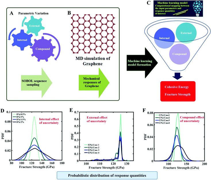
It is important to note in this context that a comprehensive Monte Carlo simulation-based probabilistic analysis is computationally exorbitant due to the involvement of thousands of MD simulations. To mitigate this problem, we exploit the emerging capabilities of machine learning, wherein the expensive MD simulations can effectively be replaced by an efficient mathematical model. In the subsequent sections, we present a concise overview of the computational methods that involve molecular dynamics simulations, machine learning algorithms, and uncertainty quantification, followed by a numerical exploration of the effects of uncertainty on the internal and external parameters of graphene along with further discussions and concluding remarks.

2. Methodology

2.1 Molecular dynamics simulations

A set of molecular dynamics simulations for the uniaxial deformation of monolayer graphene are carried out to determine the mechanical and structural characteristics of graphene. In the current analysis, we concentrate on the ultimate tensile strength and cohesive energy, as discussed in the preceding section. Here, we have elaborated the methodology for the MD simulation of pristine graphene, followed by the machine-learning-assisted uncertainty quantification in the following subsections.

For any MD simulation, implementing the proper IP plays a vital role in the prediction of mechanical responses. In the present study, MD simulations have been carried out based on the Tersoff IP. The Tersoff is a three-body potential, which refers to the potential energy between the individual atoms. The energy E between the atoms is described as

where

V_ij = f_C(r_ij)[f_R(r_ij) + b_ijf_A(r_ij)]. (2)

Here, V_ij is the potential energy of the system, while f_R and f_A are the repulsive and attractive pair potentials and f_C refers to the cut-off function. The formula extends the potential energy of all the neighboring atoms (j and k) of atom i within the cut-off radius. The parameter r_ij refers to the separation of the adjacent atoms i and j. The parameter b_ij is an empirical bond-order coefficient, where f_R and f_A can be described as

f_R = Ae^−λ₁ (3)

and

f_A = Be^−λ₂. (4)

Here, A, B, λ₁, and λ₂ are the parameters used for two-body interactions.¹⁸Table 1 presents the deterministic values of the twelve parameters of the Tersoff IP that are utilized for the current MD simulations. It can be noted that the random variation in these twelve parameters is considered as the internal sources of uncertainty in the current analysis, which will become clear at a later stage in this article.

Table 1 Internal (Tersoff IP) and external parameters (temperature and strain rate) of MD simulations considered as sources of uncertainty

Type of uncertainty source	Parameter	Deterministic value
Internal parameters (Tersoff)	γ	1.0
	A (eV)	1393.6
	B (eV)	346.74
	λ 1 (Å^−1)	3.4879
	λ 2 (Å^−1)	2.2119
	n	0.72751
	C	38 049
	β (× 10^−7)	1.5724
	D	4.3484
	H	−0.57058
	R (Å)	1.8
	D (Å)	0.15
External parameters	Temperature (K)	300
	Strain rate (ps)	0.001

---

The molecular structure of pristine graphene is developed here by utilizing an open-source platform, visual molecular dynamics (VMD).⁵⁴ Pristine graphene, of dimensions 7.2 nm (nanometers), with 2040 carbon atoms arranged in a hexagonal lattice, is considered in the present study. The data-files used for MD simulations, which contain the xyz coordinates of each atom, were generated using the topotool plugin of VMD. The MD simulations were conducted using LAMMPS,⁵⁵ an open-source code for molecular dynamics simulations. The structure of modelled graphene was subjected to periodic boundary conditions (PBCs) in each direction to eliminate the finite size effect. Prior to running the desired simulation, the structure is relaxed by minimizing the energy. We utilized a conjugate gradient method for the energy minimization, followed by a Nosé–Hoover barostat to maintain the pressure in all directions. For energy minimization and running the simulations, an integration time-step of 1 fs (femtoseconds) is used. The uniaxial tensile deformation of monolayer graphene was conducted at room temperature (∼300 K) and with a strain rate of 0.001 ps⁻¹ (per picosecond). As stated earlier, the temperature (T) and strain rate (SR) are considered as the external sources of uncertainty (refer to Table 1), which are expected to vary randomly within certain bounds in practical scenarios.

The atomistic stresses in the current study are interpreted as the virial tensor. The formulation to determine the virial stress in the LAMMPS environment is given by

The former term in the above equation consists of the virial tensor component, while the latter term consists of the kinetic energy tensor component. The superscripts α and β define the nomenclature assigned to two individual atoms in the neighborhood, while i and j provide the directional indices, m^α and v^α_i refer to the mass and velocity of the atom α, respectively. R^β_i is the location of atom β in the i direction. F^αβ_j is the force due to an atom β on atom α along the j direction. V refers to the total volume of the material system.⁴⁰ The stress outputs obtained from LAMMPS are the product of the pressure in the considered direction and the volume of the system. To obtain the directional stress components, it is essential to divide the LAMMPS derived stress values by the volume of the system. In the present study, we used the instantaneous volume to determine the directional stress component, which is given by V₀(1 + ε), where V₀ and ε stand for the original volume of the material system and the strain, respectively.⁵⁶ The stress deliverables from the LAMMPS were divided by the instantaneous volume to determine the averaged stress in the desired directions. The cohesive energy of pristine graphene, after the relaxation stage, was determined as

where E_coh, U, and N refer to the cohesive energy, the total energy of the relaxed system, and the total number of atoms in the considered system, respectively.

In this context, the importance of the time-step in general molecular dynamics simulations can be noted. However, the objective of the present study is to mainly identify the influence of parametric uncertainty (the internal and external parameters) on the fracture properties of graphene. The fracture properties of any material system are the final outcome of a continuous deformation of the structure over time. We have restricted the study to a certain timestep (1 fs) to avoid the excessive computational expense of the series of molecular dynamics simulations without affecting the output quantity of interest. A decrease in the timestep increases the number of iterations for failure of the graphene layer and makes the simulation computationally expensive.

2.2 Machine-learning model based on polynomial chaos Kriging (PCK)

Machine-learning models can form computationally efficient surrogates of expensive simulation models (such as MD simulations) for carrying out intensive iterative analyses like optimization, sensitivity analysis and uncertainty quantification.^57,58 Polynomial chaos Kriging (PCK) is a hybrid non-intrusive metamodel which combines polynomial chaos expansion (PCE) and Kriging approaches. The PCE approximates the global behavior of the computational model and Kriging manages the local variability of the responses, resulting in a better prediction capability. The mathematical form of PCK is as follows⁵⁹Here, represents the weighted sum of the orthonormal polynomials, σ² denotes the variance, and Z(x,w) contributes the zero mean. The orthonormal polynomials are given by {ψ_α(x),α ∈ A}. A⊂Ν^m is the set of selected multi indices of multivariate polynomials.

The PCK algorithm initiates with finding the optimal polynomial set of predictors utilizing the PCE framework, which ensures the polynomial set with the smallest leave-one-out (LOO) error. The universal Kriging algorithm is used once the sparse PC basis is set. At the end of the algorithm, the error is estimated using the LOO approach. The estimation of error based on LOO has the advantage over an empirical error in the sense that empirical error generally under-predicts the generalization error due to overfitting. By contrast, the error estimated using the LOO approach takes global error into account.⁶⁰ We have adopted the PCK-based hybrid machine-learning algorithm on the basis of the recent results presented in the literature, revealing the superior performance of hybrid machine-learning algorithms.⁶¹

2.3 Machine-learning-assisted Monte Carlo simulation

2.3.1 Overview of the adopted algorithm. Monte Carlo simulation (MCS) is used in the present study to perform a comprehensive probabilistic analysis for the mechanical responses of interest, wherein machine learning (ML) is integrated explicitly with the MD simulation framework for achieving computational efficiency. First, the internal and external factors that influence the desired mechanical responses of interest (fracture strength and cohesive energy in the current analysis) are recognized with the help of a set of pilot MD simulations. To this end, we integrated the PCK-based machine-learning approach with computational analysis for carrying out Monte Carlo simulations.⁵⁶

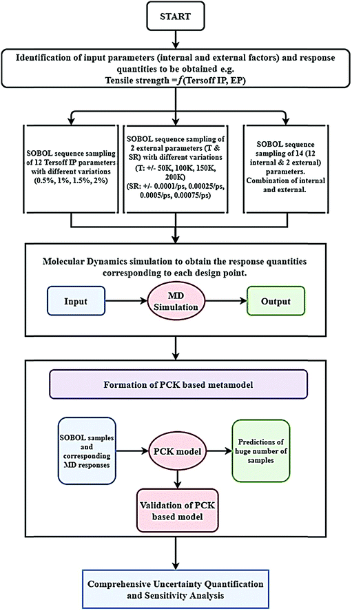
In the ML-assisted MCS approach, first the machine-learning model is formed based on an optimal set of MD simulation data, drawn from the quasi-random Sobol sequence. Subsequently, the machine- learning model is used instead of direct MD simulations for efficient prediction to obtain thousands of realizations of the Monte Carlo simulation. Before carrying out the Monte Carlo simulation, for each case (internal, external, and combined), the PCK model is formed and tested for accuracy using cross-validation based on evaluating the percentage error:

The flowchart of PCK-based machine-learning-model formation and uncertainty analysis is illustrated in Fig. 2.

Fig. 2 Flowchart of the uncertainty quantification. The figure explains formation of the machine-learning model and the subsequent uncertainty analysis of graphene.

2.3.2 Quasi-random Sobol sequence sampling. In this subsection, we provide further details of the sampling algorithm, as mentioned in the preceding subsection. The quasi-random Sobol sequence is a pseudo-random sampling technique that perturbs the considered stochastic input parameters in the desired parametric range for obtaining a predefined number of samples algorithmically. The advantage of using Sobol sequence sampling is that it captures the distribution of parameters with algorithmically generated sample points, leading to faster convergence compared with other sampling techniques.⁶³ In the present study, Sobol sequence sampling is utilized to create the sample space to perform the MD simulation and construct the hybrid machine-learning model for further uncertainty analysis.

A systematic stochastic investigation is presented here that considers the individual and compound effects of the internal and external sources of uncertainty (refer to Fig. 1 and 2). We started the investigation with a small perturbation of the IP parameters in the range of 0.5% and then increased the variation to 1%, 1.5% and 2%. Here, if θ is considered as the deterministic value of a stochastic parameter, then we define

where

Δ ∈ {0.5%,1%,1.5%,2%}

θ_i = θ_min + SP_i(θ_max − θ_min), i ∈ {1,2,3,…N} (10)

Here, Δ is the percentage variation with which the original parameters are perturbed. The range of the stochastic input parameters is defined by the difference in θ_max and θ_min. The ith realization of the perturbed parameter of the Monte Carlo simulation is determined based on eqn (10), wherein SP_i represents the Sobol parameter that lies in the random numbers drawn from the probabilistic distribution of the stochastic input parameter. In the next stage, the external parameters were perturbed within specified ranges of variabilities using different cases as shown in Table 2. It may be noted that the external parameters do not have any influence on the cohesive energy of the material. Thus, only the ultimate tensile strength is investigated for the cases involving uncertainty in the external parameters. Subsequently, the compound effect of the internal and external parameters is investigated only for the ultimate tensile strength (since the cohesive energy is not dependent on the external parameters), wherein a total of fourteen sources of uncertainties is accounted. Note that different cases arise in the compound uncertainty analysis due to the consideration of different degrees of stochasticity in the internal and external parameters, which are systematically explored in the following section.

Table 2 Cases of stochastic perturbation in the considered external parameters

Case	Temperature [T (K)]	Strain rate [SR (ps)]
Case-1	300 ± 50	0.001 ± 0.0001
Case-2	300 ± 100	0.001 ± 0.00025
Case-3	300 ± 150	0.001 ± 0.0005
Case-4	300 ± 200	0.001 ± 0.00075

---

3. Results and discussion

In the present study, the MD simulation-based deterministic analysis of graphene has been extended to the stochastic regime for carrying out a comprehensive analysis pertaining to variations in the internal parameters, external parameters and the compound effects therein. Prior to applying probabilistic methods, the output quantities of interest resulting from the MD simulation have been validated with the earlier reported results from the literature. To this end, the uniaxial deformation of monolayer graphene (7.2 × 7.2 nm²) has been conducted with a strain rate of 0.001 ps⁻¹ at a temperature of 300 K. The uniaxial deformation of graphene in its armchair direction is carried out. The fracture strength and cohesive energy of graphene are determined as a result of this deterministic simulation. Good agreement is found with the reported values published in the literature (refer to Table 3), essentially instilling the confidence required for extending the MD simulation framework to the stochastic domain. Also, four different models with dimensions of 5.2 × 5.2 nm², 7.2 × 7.2 nm², 9.2 × 9.2 nm², and 11.2 × 11.2 nm² are modeled to check the convergence of the responses as a function of the size of the graphene monolayer. The outcome of the convergence study revealed that the fracture strength of graphene has a standard deviation of 4.22 GPa, whereas the cohesive energy has the standard deviation of 0.0449 eV per atom. The results obtained by Zhang et al.⁴⁵ are in good agreement with the negligible differences in the responses obtained in the convergence study. In further analyses, a moderately sized graphene monolayer with dimensions of 7.2 × 7.2 nm² is used to keep the computational costs within acceptable bounds. In the subsequent sections involving uncertainty quantification, we will first discuss the construction and validation of the respective machine-learning models, followed by Monte Carlo simulation-based probabilistic uncertainty quantification of the response quantities of interest.

Table 3 Comparison of deterministic mechanical properties of pristine graphene obtained in the present study with the reported literature

Reference	Fracture strength (GPa)	Cohesive energy (eV per atom)
Lee et al. (AFM)^10	130 ± 10	—
Mortazavi et al. (MD, modified Tersoff)^17	132	—
Rajasekaran et al. (MD, optimized Tersoff)^21	124	—
Gupta et al. (MD, Original Tersoff)^40	195.9	—
Shin et al. (Quasi Monte Carlo)^52	—	−7.906
Dhaliwal et al. (MD, AIREBO)^35	—	−7.427
Present study (MD, Tersoff)	195.9	−7.2452

---

3.1 Uncertainty quantification of the internal parameters

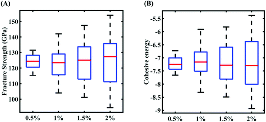
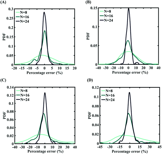
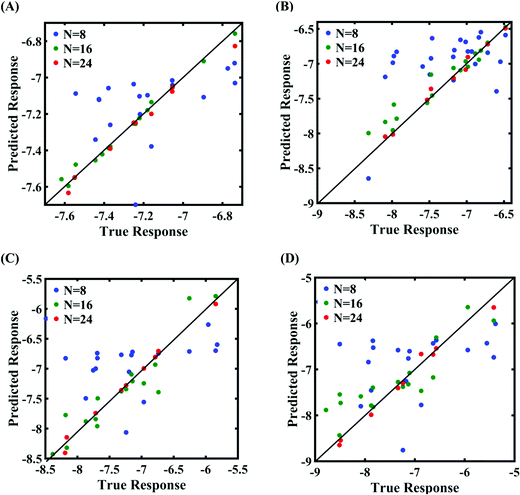
In this section, we embark on establishing machine-learning-assisted computational mapping between the uncertainties associated with the internal parameters and the level of uncertainty caused by the same in the response quantities of interest. To form the machine-learning models, Sobol sequence sampling of the parameters of the Tersoff IP (refer to Table 1) is carried out with different levels of stochastic variation (0.5%, 1%, 1.5%, and 2%) to create the design space of N = 32 samples for each case of variation. Throughout this study, the rationale for selecting the number of samples is to use as few samples as possible in order to construct a machine-learning model with an adequate performance (i.e., the prediction accuracy). Subsequently, a set of molecular simulations (in total 32 × 4 = 128 simulations) are conducted to obtain the respective fracture strength and cohesive energy for each sample. At this level, based on these 32 individual samples corresponding to each degree of stochastic variation, we obtain the bounds of the two response quantities. As a primary outcome, it is revealed from Fig. 3 that the variation in the range of fracture strength and cohesive energy gradually increases as the variation in the Tersoff IP parameters is increased.

Fig. 3 Variation in output quantities of responses subjected to the different perturbation percentages in the Tersoff IP parameters: (A) fracture strength of graphene and (B) cohesive energy of graphene.

In order to form the PCK-based machine-learning models, the MD simulation is treated as the learning source where the Tersoff IP parameters are considered as the input parameters and the responses of the MD simulations (fracture strength and cohesive energy) are considered as the output quantities. Once the PCK model is formed, it can be used to efficiently predict the output quantities of interest that correspond to any random combination of the input parameters. The available input–output dataset obtained based on MD simulations is split into training and testing sets. In general, the leave-one-out (LOO) approach can be used to test the accuracy of the machine-learning model under consideration for providing a general intuition about its performance. However, LOO is not an optimal method to validate the model as the prediction error determined using this approach tends to vary a lot in comparison with other methods. In the present study, we utilized the leave-p-out (LpO) cross-validation method, where p training points are left out at each iteration to create test data and check the performance of the machine-learning model. This validation approach has the advantage of the most optimal utilization of the set of MD simulation data. For uncertainty quantification of the internal parameters, we checked the accuracy of PCK-based metamodels by utilizing the number N of sample data (N = 8, 16, 24) as a training data set and leaving p (= 32 − N) samples for the cross-validation. Fig. 4–7 illustrate the performance and validation of PCK metamodels based on the scatter plots and error plots (using the probability density function (PDF)) for both of the considered response quantities of graphene (the fracture strength and cohesive energy), wherein different cases of variations in the Tersoff IP parameters are considered. It is noted from the figures that N = 24 training samples provide a sufficient level of accuracy in prediction for each case of stochastic variation. Moreover, the PDF (i.e., the probability distribution) for the percentage errors reveals that the probability of having a lesser error is significantly more than having a high value of error even within the bounds of the errors presented. Thus, having the required level of confidence in the prediction capability of the machine-learning models, we further investigate the probabilistic characteristics and sensitivity of the internal input parameters based on large-scale datasets, as presented in the following paragraphs.

Fig. 4 Scatter plots between the MD response and PCK metamodel with different training sample sizes (N) for the fracture strength of graphene: (A) 0.5% variation in Tersoff IP parameters, (B) 1% variation in Tersoff IP parameters, (C) 1.5% variation in Tersoff IP parameters, and (D) 2% variation in Tersoff IP parameters.

Fig. 5 Probability density function plots for percentage error of machine-learning models formed using different training sample sizes concerning the fracture strength of graphene: (A) 0.5% variation in Tersoff IP parameters (for N = 24, RMSE: 1.165), (B) 1% variation in Tersoff IP parameters (for N = 24, RMSE: 1.9932), (C) 1.5% variation in Tersoff IP parameters (for N = 24, RMSE: 4.2360), and (D) 2% variation in Tersoff IP parameters (for N = 24, RMSE: 2.5228).

Fig. 6 Scatter plots between the MD response and PCK metamodel with different training sample sizes (N) for the cohesive energy of graphene: (A) 0.5% variation in Tersoff IP parameters, (B) 1% variation in Tersoff IP parameters, (C) 1.5% variation in Tersoff IP parameters, and (D) 2% variation in Tersoff IP parameters.

Fig. 7 Probability density function plots for percentage error of machine-learning models formed using different training sample sizes concerning the cohesive energy of graphene: (A) 0.5% variation in Tersoff IP parameters (for N = 24, RMSE: 0.0308), (B) 1% variation in Tersoff IP parameters (for N = 24, RMSE: 0.0583), (C) 1.5% variation in Tersoff IP parameters (for N = 24, RMSE: 0.0713), and (D) 2% variation in Tersoff IP parameters (for N = 24, RMSE: 0.1213).

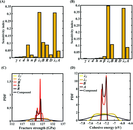
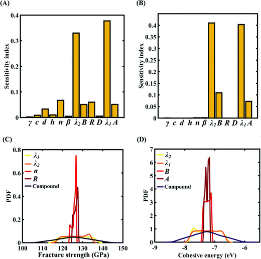
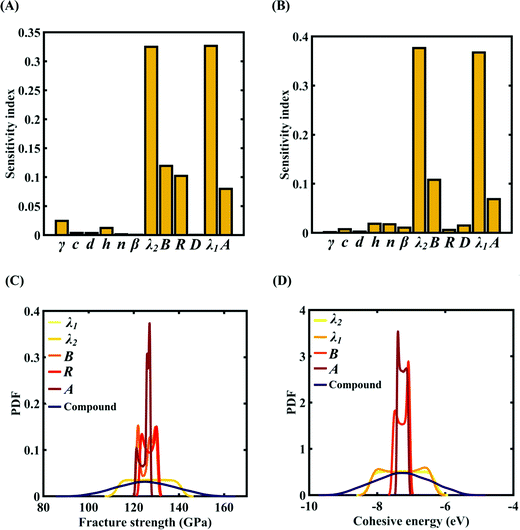
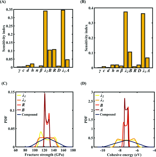
To assess the relative importance of individual Tersoff IP parameters on the response quantities, a data-driven sensitivity analysis is carried out, where 10 000 samples are generated using MCS sampling with the same range of variation as the training dataset (±0.5%, ±1%, ±1.5%, and ±2%). The relative variance of an individual input parameter is used to determine the sensitivity indices.⁶² The data-driven sensitivity analysis for all four cases of variation in Tersoff IP (refer to Fig. 8–11(A and B)) reveals that there are certain set of parameters that have a more prominent influence on the critical response variables (i.e., the fracture strength and cohesive energy). For instance, in each case of variation, the Tersoff IP parameters λ₁, λ₂, B and R were found to have more significance on the fracture strength of graphene. Similarly, the parameters λ₁, λ₂, B and A have more sensitivity on the cohesive energy of graphene.

Fig. 8 Sensitivity analysis and probabilistic characterization of the response quantities of interest using PCK-based machine-learning models considering the sample space within ±0.5% variation of the Tersoff IP parameters: (A) sensitivity analysis of the Tersoff IP parameters for the fracture strength of graphene, (B) sensitivity analysis of the Tersoff IP parameters for the cohesive energy of graphene, (C) PDF plots of the fracture strength for the individual variation in the most significant parameters of the Tersoff IP and compound variation of all the internal input parameters, and (D) PDF plots of cohesive energy for the individual variation in the most significant parameters of the Tersoff IP and compound variation of all the internal input parameters.

Fig. 9 Sensitivity analysis and probabilistic characterization of the response quantities of interest using PCK-based machine-learning models considering the sample space within ±1% variation of the Tersoff IP parameters: (A) sensitivity analysis of the Tersoff IP parameters for the fracture strength of graphene, (B) sensitivity analysis of the Tersoff IP parameters for the cohesive energy of graphene, (C) PDF plots of the fracture strength for the individual variation in the most significant parameters of the Tersoff IP and compound variation of all the internal input parameters, and (D) PDF plots of cohesive energy for the individual variation in the most significant parameters of the Tersoff IP and compound variation of all the internal input parameters.

Fig. 10 Sensitivity analysis and probabilistic characterization of the response quantities of interest using PCK-based machine-learning models considering the sample space within ±1.5% variation of the Tersoff IP parameters: (A) sensitivity analysis of the Tersoff IP parameters for the fracture strength of graphene, (B) sensitivity analysis of the Tersoff IP parameters for the cohesive energy of graphene, (C) PDF plots of the fracture strength for the individual variation in the most significant parameters of the Tersoff IP and compound variation of all the internal input parameters, and (D) PDF plots of cohesive energy for the individual variation in most the significant parameters of the Tersoff IP and compound variation of all the internal input parameters.

Fig. 11 Sensitivity analysis and probabilistic characterization of the response quantities of interest using PCK-based machine-learning models considering the sample space within ±2% variation of the Tersoff IP parameters: (A) sensitivity analysis of the Tersoff IP parameters for the fracture strength of graphene, (B) sensitivity analysis of the Tersoff IP parameters for the cohesive energy of graphene, (C) PDF plots of the fracture strength for the individual variation in the most significant parameters of the Tersoff IP and compound variation of all the internal input parameters, and (D) PDF plots of cohesive energy for the individual variation in most the significant parameters of the Tersoff IP and compound variation of all the internal input parameters.

After assessing the relative sensitivity of the Tersoff IP parameters, we exploit the machine-learning models to characterize the individual and compound probabilistic uncertainty effects of the internal input parameters (refer to Fig. 8–11(C and D)). In the case of the individual effects, we focus on the most sensitive Tersoff IP parameters for probabilistic characterization. It is noted that the response bounds corresponding to different individual stochastic effects follow the respective sensitivities, while response bounds corresponding to the compound effect of all the Tersoff IP parameters are the highest for all the considered cases. In this context, it may be noted that the probabilistic descriptions are plotted corresponding to 10 000 realizations of (machine-learning-assisted-) Monte Carlo simulation in each case, while only 24 actual MD simulations are required to perform this data-intensive analysis. Thus, we achieve a computational efficiency of more than 400 times in terms of MD simulation.

3.2 Uncertainty quantification of the external parameters

In this subsection, we focus on the effect of uncertainty concerning the external parameters such as the temperature and strain rate. Since cohesive energy is an inherent property of the material, it is not affected by the external parameters. As a consequence, this subsection is restricted to the investigation of stochastic fracture strength only. To assess the uncertainty associated with the external parameters, the parameters are perturbed with different levels of stochastic variation within the bounds indicated in Table 2. Similar to the cases of variation in the internal parameters as explained in Subsection 3.1, four different datasets (with N = 64 samples in each case) are constructed via Sobol sequence sampling considering the stochastic variations illustrated in Table 2. The MD simulations (64 × 4 = 256) are performed to determine the output quantities of interest for each instance of the sample space. A preliminary analysis concerning the range of variation in the fracture strength corresponding to different cases of variations in the external parameters is presented in Fig. 12. It can be noticed that the variation in the response quantities increases with the increasing perturbation bound of the external input parameters. However, we note that there are more outliers in the response dataset, indicating a more complex and nonlinear nature of the input–output relationship.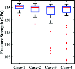

Fig. 12 Bounds of stochastic variation in the fracture strength. The range of fracture strength values under different degrees of stochastic variation in the external parameters (temperature and strain rate) is plotted. Here, the degrees of stochastic variation are presented as different cases, as defined in Table 2. It may be noted in this context that the other response quantity of interest, the cohesive energy, is independent of the stochastic external parameters. The red dots in the plot refer to the outliers available in the deterministic results. It can be noticed here that with the increase in the range of temperature and strain rate the number of outliers in the results increases.

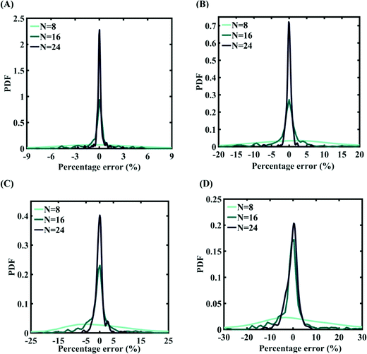
Machine-learning models are formed similar to the case of internal parameters, as presented in the preceding section. However, for the case of uncertainty in the external parameters, despite having only two input variables (strain rate and temperature), it is found that more MD simulations are required to achieve an adequate level of accuracy due to the more complex and nonlinear nature of the input–output relationship. Results concerning the prediction accuracy are presented in Fig. 13 and 14 using scatter plots and probability density function plots of error. Different sample sizes (N = 16, 32, and 48) are utilized to train the model, and the rest of the samples (p = 64 − N = 48, 32, and 16) are used for cross-validation following the LpO approach. It is noted from the figures that N = 48 training samples provide a sufficient level of accuracy in prediction. Moreover, the probability density function for the percentage errors reveals that the probability of having a lesser error is significantly more than having a high value of error even within the bounds of errors presented. Thus, having the required level of confidence in the prediction capability of the machine-learning models, we further investigate the probabilistic characteristics and sensitivity of the external input parameters based on large-scale datasets, as presented in the following paragraphs.

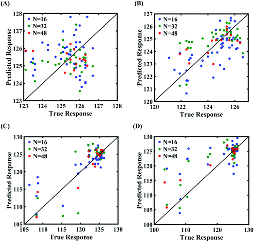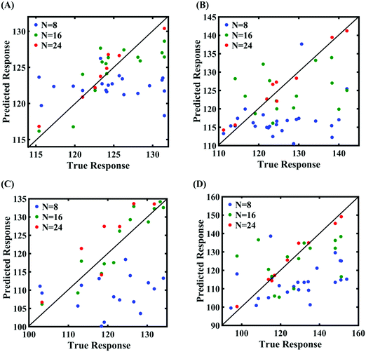
Fig. 13 Scatter plots between the MD response and the PCK metamodel with different training sample sizes (N) for the fracture strength of graphene: (A) 300 ± 50 K, 0.001 ± 0.0001 ps⁻¹ variation in temperature and strain rate, (B) 300 ± 100 K, 0.001 ± 0.00025 ps⁻¹ variation in temperature and strain rate, (C) 300 ± 150 K, 0.001 ± 0.0005 ps⁻¹ variation in temperature and strain rate, and (D) 300 ± 200 K, 0.001 ± 0.00075 ps⁻¹ variation in temperature and strain rate (refer to Table 2 for further details regarding the considered stochastic input bounds for the external parameters).

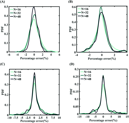Fig. 14 Probability density function plots for the percentage error of machine-learning models formed using different training sample sizes concerning the fracture strength of graphene: (A) Case-1: 300 ± 50 K and 0.001 ± 0.0001 ps⁻¹ variation in temperature and strain rate (for N = 48, RMSE: 1.5198), (B) Case-2: 300 ± 100 K and 0.001 ± 0.00025 ps⁻¹ variation in temperature and strain rate (for N = 48, RMSE: 1.5417), (C) Case-3: 300 ± 150 K and 0.001 ± 0.0005 ps⁻¹ variation in temperature and strain rate (for N = 48, RMSE: 2.215), and (D) Case-4: 300 ± 200 K and 0.001 ± 0.00075 ps⁻¹ variation in temperature and strain rate (for N = 48, RMSE: 3.3227) (refer to Table 2 for further details of the considered stochastic input bounds for the external parameters).

To assess the relative importance of individual external parameters on the fracture strength, a data-driven sensitivity analysis is carried out, where 10 000 samples are generated using SOBOL sequence sampling with the same range of variation as the training dataset as given in Table 2. The relative variance of an individual input parameter is used to determine the sensitivity indices. The data-driven sensitivity analysis for all four cases of variation (refer to Fig. 15) reveals that temperature is more sensitive than strain rate. After assessing the relative sensitivity of strain rate and temperature, we exploit the machine-learning models to characterize the individual and compound probabilistic uncertainty effects of the external input parameters (refer to Fig. 16). It is noted that the response bounds corresponding to different individual stochastic effects follow the respective sensitivities, while response bounds corresponding to the compound effect are the highest for all the considered cases. Similar to the case of uncertainty in the internal parameters, it may be noted that the probabilistic descriptions are plotted corresponding to 10 000 realizations of (machine-learning-assisted-) Monte Carlo simulation in each case, while only 48 actual MD simulations are required to perform this data-intensive analysis. Thus, for the case of external uncertainty quantification, we achieve a computational efficiency of more than 200 times in terms of MD simulation.

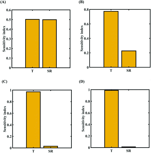Fig. 15 Data-driven sensitivity analysis of external parameters corresponding to the fracture strength of graphene using PCK-based machine-learning models (refer to Table 2 for cases of variation in the external parameters): (A) Case-1: 300 ± 50 K and 0.001 ± 0.0001 ps⁻¹ variation in temperature and strain rate, (B) Case-2: 300 ± 100 K and 0.001 ± 0.00025 ps⁻¹ variation in temperature and strain rate, (C) Case-3: 300 ± 150 K and 0.001 ± 0.0005 ps⁻¹ variation in temperature and strain rate, and (D) Case-4: 300 ± 200 K and 0.001 ± 0.00075 ps⁻¹ variation in temperature and strain rate.

Fig. 16 Probability density function (PDF) plots of the fracture strength of graphene with respect to the variation in individual parameters and compound variation: (A) Case-1: 300 ± 50 K and 0.001 ± 0.0001 ps⁻¹ variation in temperature and strain rate, (B) Case-2: 300 ± 100 K and 0.001 ± 0.00025 ps⁻¹ variation in temperature and strain rate, (C) Case-3: 300 ± 150 K and 0.001 ± 0.0005 ps⁻¹ variation in temperature and strain rate, and (D) Case-4: 300 ± 200 K and 0.001 ± 0.00075 ps⁻¹ variation in temperature and strain rate. The insets illustrated in the (C) and (D) demonstrate the variation in the fracture strength of the graphene with respect to the individual stochastic variation in temperature (T) and strain rate (SR).

3.3 Uncertainty quantification of the compound effect of internal and external parameters

We have investigated the effect of uncertainty in the internal and external parameters separately in the two preceding subsections. However, to quantify the effect of uncertainty in a more realistic and practically relevant framework, it is essential to account for the effect of uncertainty in the internal and external parameters simultaneously. Keeping in mind that the cohesive energy is not influenced by external uncertainty, we focus on the fracture strength while quantifying the compound effect of internal and external uncertainty. An analysis space of the fourteen input parameters (twelve Tersoff IP parameters and two external parameters) is considered with different degrees of uncertainty in the internal and external parameters as shown in Table 4. At this level, based on 64 samples corresponding to each degree of stochastic variation, we obtain the bounds of the fracture strength. As a primary outcome, it is revealed from Fig. 17 that the variation in the range of fracture strength gradually increases as the variation in the internal and external parameters is increased.

Table 4 Compound cases of stochastic perturbation (Case-A to Case-D) considering the internal parameters (IPs) and external parameters (EPs). Different individual cases (Case-1 to Case-4) of the EP are depicted in Table 2

Case	Compound effect of stochastic Perturbation
Case-A	IP@ ±0.5%	EP@Case-1
Case-B	IP@ ±1%	EP@Case-2
Case-C	IP@ ±1.5%	EP@Case-3
Case-D	IP@ ±2%	EP@Case-4

---

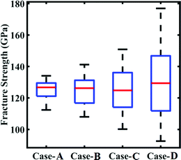Fig. 17 Bounds of stochastic variation in the fracture strength under the influence of compound uncertainty. The range of fracture strength under different degrees of stochastic variation in the internal and external parameters (refer to Table 4) is plotted.

Machine-learning models are formed for the fracture strength, similar to the earlier cases, as presented in Subsections 3.1 and 3.2. Results concerning the prediction accuracy are presented in Fig. 18 and 19 using scatter plots and probability density function plots of error, respectively. Different sample sizes (N) are utilized to train the model, and the rest of the samples are used for cross-validation following the LpO approach. It is noted from the figures that N = 48 training samples provide a sufficient level of accuracy in prediction for cases A and B (refer to Table 4). However, 48 samples were not found sufficient to construct the model with an acceptable predictive accuracy (% error ≈ ±20%) for case C and case D. To this end, we gradually increased the sample size up to 96 samples until the errors were minimized to acceptable limits (refer to Fig. 19(C) and (D)). Similar to the earlier cases, the probability density function for the percentage errors reveals that the probability of having a lesser error is significantly more than having a high value of error, even within the bounds of the errors presented. Thus, having the required level of confidence in the prediction capability of the machine-learning models, we further investigate the probabilistic characteristics and sensitivity of the compound effect of the internal and external input parameters based on large-scale datasets, as presented in the following paragraphs.

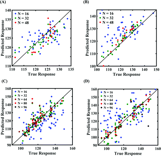Fig. 18 Scatter plots between the MD response and the PCK metamodel with different training sample sizes (N) for the fracture strength of graphene: (A) compound variation of Case- A, (B) compound variation of Case-B, (C) compound variation of Case-C, and (D) compound variation of Case-D (refer to Table 4 for further details regarding the considered stochastic input bounds for the compound variation cases).

Fig. 19 Probability density function plots for the percentage error of machine-learning models formed using different training sample sizes concerning the fracture strength of graphene: (A) compound variation of Case-A (for N = 48, RMSE: 1.055), (B) compound variation of Case-B (for N = 48, RMSE: 0.00075), (C) compound variation of Case-C (for N = 48, RMSE: 0.6745), and (D) compound variation of Case-D (for N = 48, RMSE: 1.9588) (refer to Table 4 for further details regarding the considered stochastic input bounds for the compound variation cases).

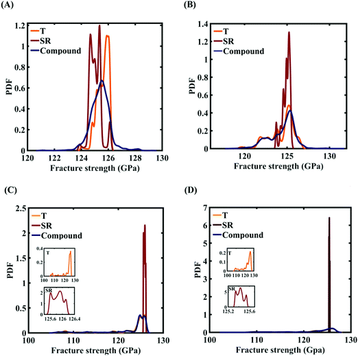
To assess the relative importance of individual internal and external parameters on the fracture strength, a data-driven sensitivity analysis is carried out, where the 10 000 samples are generated using Sobol sequence sampling with the same range of variation as for the training dataset as given in Table 4. The relative variance of an individual input parameter is used to determine the sensitivity indices. The data-driven sensitivity analysis for all four cases of variation (refer to Fig. 20) reveals that λ₁ and λ₂ are the most sensitive parameters among all the internal and external input parameters. It can also be noticed that the compound sensitivity of all the internal parameters is significantly higher than the compound sensitivity of all the external parameters. After assessing the relative sensitivity of the internal and external input parameters, we exploit the machine-learning models to characterize the individual (for the most sensitive parameters) and compound probabilistic uncertainty effects (refer to Fig. 21). It is noted that the response bounds corresponding to the different individual stochastic effects follow the respective sensitivities, while response bounds corresponding to the compound effect are the highest for all the considered cases. It may be noted in this context that the probabilistic descriptions are plotted corresponding to 10 000 realizations of (machine-learning-assisted-) Monte Carlo simulation in each case, while only 48 (or 96) actual MD simulations are required to perform this data-intensive analysis. Thus, we achieve a computational efficiency of more than 200 (100 for case C and case D) times here in terms of the expensive MD simulations.

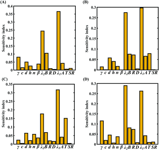Fig. 20 Data-driven sensitivity analysis of internal and external parameters corresponding to the fracture strength of graphene using PCK-based machine-learning models: (A) Case-A, (B) Case-B, (C) Case-C, and (D) Case-D (refer to Table 4 for detailed information regarding the cases of variation).

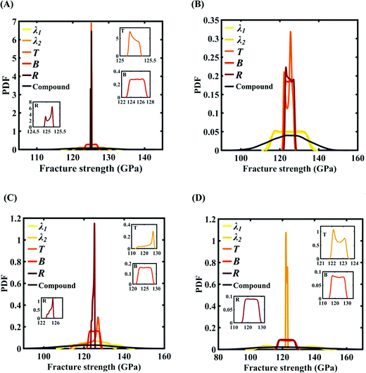Fig. 21 Probability density function (PDF) plots for the fracture strength of graphene with respect to the variation in individual parameters (for the five most sensitive parameters) and compound variation: (A) Case-A, (B) Case-B, (C) Case-C, and (D) Case-D (refer to Table 4 for descriptions of all the cases). The influence of the individual stochastic variation in the parameters R, B, and T on the fracture strength of graphene is illustrated in the insets provided in (A), (C), and (D).

To summarize the numerical results presented in this section, we would like to highlight to the readers that we have addressed the effects of both internal and external uncertainty. Moreover, as a machine-learning-based approach is adopted, it is crucially important to validate the prediction capability of the machine-learning models for both internal and external uncertainties. Subsequently, results on uncertainty quantification and sensitivity analysis are presented in this article. Thus, we would like to emphasize the vast scope of this paper that warrants plotting multiple numerical results (as presented in this section).

1. Three forms of analyses are presented considering internal uncertainty, external uncertainty and the compound effect of these uncertainties. Along with these, an in-depth deterministic analysis is presented to portray the fundamental physics of the problem.

2. For each of the above three cases, two different response quantities of interest (the fracture strength and cohesive energy) are investigated.

3. We have adopted a machine-learning-assisted molecular dynamics simulation approach in this investigation. Validation and convergence studies of output parameters of interest are critically important before exploiting the machine-learning models for further predictions and analyses. Unless all the considered cases are validated, enough confidence in the subsequent uncertainty quantification cannot be obtained. Interestingly, all these results differ significantly from each other depending on the number of input parameters and degree of complexity in the input–output mapping. The plots shown in Fig. 4–7 are associated with the four different ML models trained with the four different sample spaces (N = 32 samples for each), which are constructed by perturbing the Tersoff IP parameters with 0.5%, 1%, 1.5% and 2% variation. Similarly, Fig. 13 and 14 are associated with the four different ML models trained with the four different sample spaces (N = 64 samples for each), which are constructed by perturbing the external parameters (the temperature and strain rate) with the variations shown in Table 2. Lastly, for the cases of compound variation, four different ML models are trained with the four different sample spaces, which are constructed by implementing variations in both the internal and external parameters as shown in Table 4.

4. After validating the machine-learning-based framework extensively, we present uncertainty quantification and sensitivity analyses for internal uncertainty, external uncertainty and the compound effect of these uncertainties. In this context, we have considered different degrees of uncertainty for a comprehensive understanding. In total, 712 MD simulations are performed in the present study. The simulations are performed in three batches (variation in the internal parameters (128 simulations), variation in the external parameters (256 simulations), and combined variation (328 simulations)). The wall time of one simulation in one batch is 24 minutes, and the wall time for individual simulations in the second batch varies from 24 minutes to 55 minutes (as the strain rate is varying and time of fracture of graphene varies accordingly), and wall time of individual simulations in the third batch varies similarly as for the second batch. Note that we have carried out the Monte Carlo simulations based on tens of thousands of simulations depending on these MD simulations by adopting the ML-assisted approach.

Conclusions and perspective

In this article, we have systematically investigated the effect of uncertainties associated with the internal parameters (the Tersoff IP parameters) and external parameters (the temperature and strain rate), both individually and via their compound effect on the mechanical properties of graphene. The Tersoff potential is extensively utilized to perform MD simulations of graphene, where the results significantly depend on the inter-atomic potential (IP) used for the specific analysis. These IP values are calibrated using the experimental data or the data received from ab initio methods to mimic certain properties of the system under consideration. When the simulations are conducted for the observations beyond the calibrated envelope of these IPs, the validity of the predicted results is questionable. In general, there is always a degree of uncertainty associated with the values of inter-atomic potentials, which could significantly influence the outcome of the MD simulations. Moreover, there are several other stochastic external factors, like the temperature and strain rate, that affect the predicted MD responses of graphene. Here we have quantified the effect of such internal and external uncertainties following a Monte Carlo simulation-based probabilistic study. In establishing the complete probabilistic descriptions of the response quantities that correspond to the different levels of source uncertainties, we show that a coupled machine-learning-based approach could lead to a significant level of computational efficiency (∼200 to 400 times). In this context, it may be noted that the input–output mapping in the case of the external parameters is more complex compared with that of the internal parameters.

The study reveals that internal parameters are more sensitive compared with the external parameters in general. Among the inter-atomic parameters, λ₁ and λ₂ are found to be the most sensitive, while temperature is more sensitive than the strain rate among the external parameters. Among the output system responses, the cohesive energy is noted to be dependent only on the inter-atomic potential parameters, while the fracture strength depends on both the internal and external input parameters. The stochastic bounds that correspond to the effect of individual uncertainties of the input parameters follow the respective sensitivities. Stochastic bounds for the compound cases are found to be significantly higher compared with the individual effects. The results show that the probabilistic descriptions are significantly more skewed towards the mean values, leading to a generalized Gaussian nature.

The novelty and scientific contributions of this article lie in developing a machine-learning-assisted molecular dynamics approach that leads to deep computational insight into the mechanical behaviour of graphene using large-scale, yet efficient, simulations that involve the individual and compound effects of the critical internal and external factors. The results of this investigation reveal that the mechanical properties of graphene can significantly deviate under the compound effect of source-uncertainties. The numerically quantifiable outcomes of this study will improve and bring new perspectives to the inclusive mechanical design of various graphene-based devices and systems. Moreover, the proposed simulation approaches can be extended further to other 2D materials for efficient, large-scale, computational characterization including the effect of inherent uncertainties.

Conflicts of interest

The authors declare no conflicts of interest.

Acknowledgements

KKG is grateful for the financial support from MoE, India during the research work. TM acknowledges the initiation grants received from IIT Kanpur.

References

1. M. D. Dai, C. W. Kim and K. Eom, Nonlinear vibration behavior of graphene resonators and their applications in sensitive mass detection, Nanoscale Res. Lett., 2012, 7(1), 499.
2. T. Kuila, S. Bose, P. Khanra, A. K. Mishra, N. H. Kim and J. H. Lee, Recent advances in graphene-based biosensors, Biosens. Bioelectron., 2011, 26(12), 4637–4648.
3. S. Stankovich, D. A. Dikin, G. H. Dommett, K. M. Kohlhaas, E. J. Zimney, E. A. Stach and R. S. Ruoff, Graphene-based composite materials, Nature, 2006, 442(7100), 282–286.
4. V. B. Mohan, K. T. Lau, D. Hui and D. Bhattacharyya, Graphene-based materials and their composites: a review on production, applications and product limitations, Composites, Part B, 2018, 142, 200–220.
5. G. Wang, B. Wang, X. Wang, J. Park, S. Dou, H. Ahn and K. Kim, Sn/graphene nanocomposite with 3D architecture for enhanced reversible lithium storage in lithium ion batteries, J. Mater. Chem., 2009, 19(44), 8378–8384.
6. T. Mukhopadhyay, A. Mahata, S. Naskar and S. Adhikari, Probing the Effective Young's Modulus of ‘Magic Angle’ Inspired Multi-Functional Twisted Nano- Heterostructures, Adv. Theory Simul., 2020, 3(10), 2000129.
7. M. A. Amani, F. Ebrahimi, A. Dabbagh, A. Rastgoo and M. M. Nasiri, A machine learning-based model for the estimation of the temperature-dependent moduli of graphene oxide reinforced nanocomposites and its application in a thermally affected buckling analysis, Engineering with Computers, 2021, 37(3), 2245–2255.
8. Y. Chandra, S. Adhikari and E. S. Flores, Advances in finite element modelling of graphene and associated nanostructures, Mater. Sci. Eng., R, 2020, 140, 100544.
9. V. Khanna, V. Kumar and S. A. Bansal, Mechanical Properties of Aluminium- Graphene/Carbon Nanotubes (CNTs) Metal Matrix Composites: Advancement, Opportunities and Perspective, Mater. Res. Bull., 2021, 138, 111224.
10. C. Lee, X. Wei, J. W. Kysar and J. Hone, Measurement of the elastic properties and intrinsic strength of monolayer graphene, Science, 2008, 321(5887), 385–388.
11. B. Mortazavi and G. Cuniberti, Atomistic modeling of mechanical properties of polycrystalline graphene, Nanotechnology, 2014, 25(21), 215704.
12. K. K. Gupta and S. Dey ( 2019). Effect of Temperature on the Fracture Strength of Perfect and Defective MonoLayered Graphene. Advances in Computational Methods in Manufacturing, Springer, Singapore, pp. 793–804.
13. K. K. Gupta, A. Roy and S. Dey ( 2020). Comparative Study of Various Defects in Monolayer Graphene Using Molecular Dynamics Simulation. Advances in Applied Mechanical Engineering, Springer, Singapore, pp. 539–546.
14. K. Saumya, K. K. Gupta, A. Roy and S. Dey, Effect of spatial distribution of nanopores on mechanical properties of mono layer graphene, IOP Conf. Ser.: Mater. Sci. Eng., IOP Publishing, 2020, 8721, 012187.
15. V. K. Majeti, A. Roy, K. K. Gupta and S. Dey, Effect of silicon dopant on mechanical properties of monolayer graphene, IOP Conf. Ser.: Mater. Sci. Eng., IOP Publishing, 2020, 8721, 012188.
16. J. L. Tsai and J. F. Tu, Characterizing mechanical properties of graphite using molecular dynamics simulation, Mater. Des., 2010, 31(1), 194–199.
17. B. Mortazavi, Z. Fan, L. F. C. Pereira, A. Harju and T. Rabczuk, Amorphized graphene: a stiff material with low thermal conductivity, Carbon, 2016, 103, 318–326.
18. J. Tersoff, New empirical approach for the structure and energy of covalent systems, Phys. Rev. B: Condens. Matter Mater. Phys., 1988, 37(12), 6991.
19. R. Ansari, S. Ajori and B. Motevalli, Mechanical properties of defective single- layered graphene sheets via molecular dynamics simulation, Superlattices Microstruct., 2012, 51(2), 274–289.
20. Z. Ni, H. Bu, M. Zou, H. Yi, K. Bi and Y. Chen, Anisotropic mechanical properties of graphene sheets from molecular dynamics, Phys. B, 2010, 405(5), 1301–1306.
21. G. Rajasekaran, R. Kumar and A. Parashar, Tersoff potential with improved accuracy for simulating graphene in molecular dynamics environment, Mater. Res. Express, 2016, 3(3), 035011.
22. L. Lindsay and D. A. Broido, Optimized Tersoff and Brenner empirical potential parameters for lattice dynamics and phonon thermal transport in carbon nanotubes and graphene, Phys. Rev. B: Condens. Matter Mater. Phys., 2010, 81(20), 205441.
23. Y. Wang, Uncertainty in materials modeling, simulation, and development for ICME, Proc. 2015 Mater. Sci. Technol., 2015.
24. P. N. Patrone and A. Dienstfrey, Uncertainty quantification for molecular dynamics, Rev. Comput. Chem., 2018, 31, 115–169.
25. X. Zhou and S. M. Foiles, Uncertainty quantification and reduction of molecular dynamics models, Uncertainty Quantification and Model Calibration, 2017, 89.
26. Z. Wang, S. Safarkhani, G. Lin and X. Ruan, Uncertainty quantification of thermal conductivities from equilibrium molecular dynamics simulations, Int. J. Heat Mass Transfer, 2017, 112, 267–278.
27. P. Angelikopoulos, C. Papadimitriou and P. Koumoutsakos, Bayesian uncertainty quantification and propagation in molecular dynamics simulations: a high performance computing framework, J. Chem. Phys., 2012, 137(14), 144103.
28. M. J. Zimoń, R. Sawko, D. R. Emerson and C. Thompson, Uncertainty Quantification at the Molecular–Continuum Model Interface, Fluids, 2017, 2(1), 12.
29. R. A. Messerly, T. A. Knotts IV and W. V. Wilding, Uncertainty quantification and propagation of errors of the Lennard-Jones 12-6 parameters for n-alkanes, J. Chem. Phys., 2017, 146(19), 194110.
30. A. Mahata and T. Mukhopadhyay, Probing the chirality-dependent elastic properties and crack propagation behavior of single and bilayer stanene, Phys. Chem. Chem. Phys., 2018, 20(35), 22768–22782.
31. T. Mukhopadhyay, A. Mahata, S. Adhikari and M. A. Zaeem, Probing the shear modulus of two-dimensional multiplanar nanostructures and heterostructures, Nanoscale, 2018, 10(11), 5280–5294.
32. T. Mukhopadhyay, A. Mahata, S. Adhikari and M. A. Zaeem, Effective mechanical properties of multilayer nano-heterostructures, Sci. Rep., 2017, 7(1), 1–13.
33. T. Mukhopadhyay, A. Mahata, S. Adhikari and M. A. Zaeem, Effective elastic properties of two dimensional multiplanar hexagonal nanostructures, 2D Mater., 2017, 4(2), 025006.
34. G. Dhaliwal, P. B. Nair and C. V. Singh, Uncertainty and sensitivity analysis of mechanical and thermal properties computed through Embedded Atom Method potential, Comput. Mater. Sci., 2019, 166, 30–41.
35. G. Dhaliwal, P. B. Nair and C. V. Singh, Uncertainty analysis and estimation of robust AIREBO parameters for graphene, Carbon, 2019, 142, 300–310.
36. A. Agius Anastasi, K. Ritos, G. Cassar and M. K. Borg, Mechanical properties of pristine and nanoporous graphene, Mol. Simul., 2016, 42(18), 1502–1511.
37. Y. Y. Zhang and Y. Gu, Mechanical properties of graphene: Effects of layer number, temperature and isotope, Comput. Mater. Sci., 2013, 71, 197–200.
38. M. A. N. Dewapriya, R. K. N. D. Rajapakse and A. S. Phani, Atomistic and continuum modelling of temperature-dependent fracture of graphene, Int. J. Fract., 2014, 187(2), 199–212.
39. M. A. N. Dewapriya and R. K. N. D. Rajapakse, Molecular dynamics simulations and continuum modeling of temperature and strain rate dependent fracture strength of graphene with vacancy defects, J. Appl. Mech., 2014, 81(8), 081010.
40. K. K. Gupta, T. Mukhopadhyay, A. Roy and S. Dey, Probing the compound effect of spatially varying intrinsic defects and doping on mechanical properties of hybrid graphene monolayers, J. Mater. Sci. Technol., 2020, 50, 44–58.
41. T. Mukhopadhyay, A. Mahata, S. Dey and S. Adhikari, Probabilistic analysis and design of HCP nanowires: an efficient surrogate based molecular dynamics simulation approach, J. Mater. Sci. Technol., 2016, 32(12), 1345–1351.
42. A. Mahata, T. Mukhopadhyay and S. Adhikari, A polynomial chaos expansion based molecular dynamics study for probabilistic strength analysis of nano-twinned copper, Mater. Res. Express, 2016, 3(3), 036501.
43. H. Yang, et al., Machine learning and artificial neural network prediction of interfacial thermal resistance between graphene and hexagonal boron nitride, Nanoscale, 2018, 10.40, 19092–19099.
44. X. Wang, D. Han, Y. Hong, H. Sun, J. Zhang and J. Zhang, Machine learning enabled prediction of mechanical properties of tungsten disulfide monolayer, ACS Omega, 2019, 4(6), 10121–10128.
45. Z. Zhang, Y. Hong, B. Hou, Z. Zhang, M. Negahban and J. Zhang, Accelerated discoveries of mechanical properties of graphene using machine learning and high- throughput computation, Carbon, 2019, 148, 115–123.
46. J. Shi, L. Chu and R. Braun, A Kriging Surrogate Model for Uncertainty Analysis of Graphene Based on a Finite Element Method, Int. J. Mol. Sci., 2019, 20(9), 2355.
47. K. K. Gupta, T. Mukhopadhyay, A. Roy, L. Roy and S. Dey, Sparse machine learning assisted deep computational insights on the mechanical properties of graphene with intrinsic defects and doping, J. Phys. Chem. Solids, 2021, 155, 110111.
48. M. Y. Shen, T. Y. Chang, T. H. Hsieh, Y. L. Li, C. L. Chiang, H. Yang and M. C. Yip, Mechanical properties and tensile fatigue of graphene nanoplatelets reinforced polymer nanocomposites, J. Nanomater., 2013, 2013.
49. H. Kashani, Y. Ito, J. Han, P. Liu and M. Chen, Extraordinary tensile strength and ductility of scalable nanoporous graphene, Sci. Adv., 2019, 5(2), eaat6951.
50. Y. Liu, B. Xie, Z. Zhang, Q. Zheng and Z. Xu, Mechanical properties of graphene papers, J. Mech. Phys. Solids, 2012, 60(4), 591–605.
51. M. Q. Le, Cohesive energy in graphene/MoS₂ heterostructures, Meccanica, 2017, 52(1–2), 307–315.
52. H. Shin, S. Kang, J. Koo, H. Lee, J. Kim and Y. Kwon, Cohesion energetics of carbon allotropes: Quantum Monte Carlo study, J. Chem. Phys., 2014, 140(11), 114702.
53. S. J. Clark (2003). Cohesive energies. Retrieved from: http://cmt.dur.ac.uk/sjc/thesis_ppr/node50.html.
54. W. Humphrey, A. Dalke and K. Schulten, VMD: visual molecular dynamics, J. Mol. Graphics, 1996, 14(1), 33–38.
55. S. Plimpton, Fast parallel algorithms for short-range molecular dynamics, J. Comput. Phys., 1995, 117(1), 1–19.
56. A. P. Thompson, S. J. Plimpton and W. Mattson, General formulation of pressure and stress tensor for arbitrary many-body interaction potentials under periodic boundary conditions, J. Chem. Phys., 2009, 131(15), 154107.
57. N. Ganesh, P. Dutta, M. Ramachandran, A. K. Bhoi and K. Kalita, Robust metamodels for accurate quantitative estimation of turbulent flow in pipe bends, Eng. Computers, 2019, 36, 1041–1058.
58. Vaishali, T. Mukhopadhyay, R. R. Kumar and S. Dey, Probing the multi-physical probabilistic dynamics of a novel functional class of hybrid composite shells, Compos. Struct., 2021, 262, 113294.
59. R. Schobi, B. Sudret and J. Wiart, Polynomial-chaos-based Kriging, Int. J. Uncertainty Quantification, 2015, 5(2), 171–193.
60. R. Schöbi, P. Kersaudy, B. Sudret and J. Wiart (2014). Combining polynomial chaos expansions and kriging.
61. T. Mukhopadhyay, S. Naskar, S. Chakraborty, P. K. Karsh, R. Choudhury and S. Dey, Stochastic Oblique Impact on Composite Laminates: A Concise Review and Characterization of the Essence of Hybrid Machine Learning Algorithms, Archives Comput. Methods Eng., 2020, 1–30.
62. T. Mukhopadhyay, P. K. Karsh, B. Basu and S. Dey, Machine learning based stochastic dynamic analysis of functionally graded shells, Compos. Struct., 2020, 237, 111870.
63. T. Mukhopadhyay, A multivariate adaptive regression splines based damage identification methodology for web core composite bridges including the effect of noise, J. Sandwich Struct. Mater., 2018, 20(7), 885–903.
64. M. C. Trinh and T. Mukhopadhyay, Semi-analytical atomic-level uncertainty quantification for the elastic properties of 2D materials, Mater. Today Nano, 2021, 15, 100126.

---