New formulation of the theory of thermoelectric generators operating under constant heat flux
Received
5th October 2021
, Accepted 22nd November 2021
First published on 22nd November 2021
Abstract
The current theory of thermoelectric generators can only deal with situations where a thermoelectric generator operates under a constant temperature difference. In this paper, a new theoretical formulation is reported that can be applied to situations where a thermoelectric generator operates under constant heat flux, completing the thermoelectric generator theory that has been absent for more than half a century. Central to the development of this new theory is a thermoelectric relationship that links the temperature difference across a thermoelectric generator in an open circuit to that in a closed circuit, enabling new formulation. This new theory offers the capacity to calculate the maximum power output and maximum conversion efficiency of a thermoelectric generator that operates under a constant heat flux, which represents the typical characteristics of the majority of heat sources and is anticipated to have a significant impact on the design and optimization of many practical thermoelectric generators. Moreover, the theory lays the foundation for a deep understanding of the unique characteristics of thermoelectric I–V curves and opens up a new way to investigate and evaluate the thermoelectric properties and performances using the I–V curves. Other foreseeable outcomes due to this new theory include the development of a novel thermoelectric characterisation technique based on thermoelectric I–V curves, a variable thermal resistance for heat regulation and exploring the possibility of improving the performance of thermoelectric generators by pulse mode operation.
Broader context
Thermoelectric generators produce electricity by scavenging waste heat from various thermal resources. They have the potential to play a role in decarbonisation of electricity and heat and moving towards a net-zero world. To assess the viability of thermoelectric power systems, a complete theoretical model is crucial. The current theory of thermoelectric generators was developed in the 1940s, which has played an important role in developing modern thermoelectrics. However, the current theory has a drawback: it can only deal with systems operating under a constant temperature difference. For systems operating under constant heat flux, the theory becomes ineffective. Since many heat sources exhibit the feature of constant heat flux, there is an increasing demand for a theory that can deal with the operation under constant heat flux. Theoretical complexity associated with this request has been a main obstacle to the progress. The situation changed recently due to advances in two aspects: dramatically increased computing power and discovery of a key thermoelectric relationship, enabling the completion of the remaining part of the theory that has been absent for more than half a century. With the addition of this work, the theory of thermoelectric generators is now able to deal with both types of heat sources.
|
1. Introduction
The theory of thermoelectric generators operating under a constant temperature difference is well established and has played an important role in the development of thermoelectrics.1 It provides a theoretical basis for determining the performances of thermoelectric generators such as the power output and conversion efficiency. It has been widely employed for the design and optimization of thermoelectric generators.2,3 An improved model that takes into account the electrical and thermal contact resistances provides further capability for device geometry optimization.4 Based on these available theoretical frameworks, practical thermoelectric generators can be conveniently designed with their performances predicted to a sufficient accuracy. The only drawback is the requirement of prerequisite knowledge on the temperature difference across a thermoelectric generator, which also needs to be maintained constant during the operation. The theoretical procedure becomes hugely inconvenient if the temperature difference across a thermoelectric generator cannot be maintained constant.
With increasing interest in thermoelectric energy harvesting using various heat sources,5–8 it is becoming apparent that not all heat sources can maintain a constant temperature. A typical example is the thermal energy collected from solar irradiation with an absorber. When it is used to power a thermoelectric generator, the temperature of the heat source (thermal absorber) changes depending on the properties and geometry of the thermoelectric generator. In general, heat sources can be broadly divided into two types –heat sources with constant temperature and heat sources with constant heat flux (analogous to constant voltage sources and constant current sources, respectively). Thermoelectric generators behave differently upon application of different types of heat sources. For example, if the temperature difference across a thermoelectric generator can be held constant by a heat source, the heat flux through the thermoelectric generator must increase when the load resistance is reduced. On the other hand, if a heat source can maintain a constant heat flux through the thermoelectric generator, its temperature difference must decrease if the load resistance is reduced (see Section 6.1 for details). The theoretical framework for dealing with the operation under constant temperature has long been established. However, the theory for dealing with constant heat flux is still absent. The work reported in this paper was the result of an attempt to address this challenge.
2. Established theory for operation under a constant temperature difference
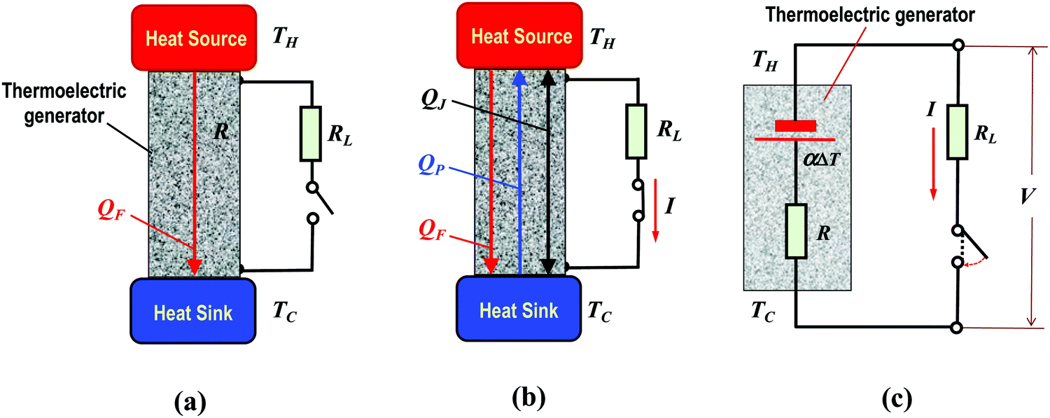
In order to understand the motivation for the reformulation of the thermoelectric theory, a brief review of the established theory of thermoelectric generators is needed. Fig. 1 shows the schematic diagram of a simplistic thermoelectric generator and its equivalent circuit. Based on this model and neglecting the electrical and thermal contact resistances at interfaces, the power output and conversion efficiency of a thermoelectric generator is given by1| |  | (1) |
| |  | (2) |
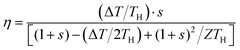
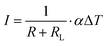
where s (=RL/R) is the ratio of the load resistance (RL) to the internal resistance of the thermoelectric generator (R); α is the Seebeck coefficient; Z (=α2σ/λ) is the figure-of-merit of the thermoelectric material; σ is the electrical conductivity and λ is the thermal conductivity; TH and TC are the temperatures at the hot and cold sides, respectively; ΔT (=TH–TC) is the temperature difference across the thermoelectric device. It can be seen that the power output and conversion efficiency are dependent on the resistance ratio s. For a given temperature difference, the maximum power output and the maximum conversion efficiency can be obtained corresponding to the optimal values of s = 1 and  , respectively1
| | 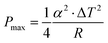 | (3) |
| | 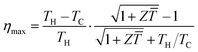 | (4) |
where ![[T with combining macron]](https://www.rsc.org/images/entities/i_char_0054_0304.gif) = (TH + TC)/2 is the average temperature across the thermoelectric generator. Eqn (4) has been widely used to estimate the efficiency of thermoelectric generators for given operating temperatures. More significantly, eqn (4) shows the importance of the material property Z for achieving high conversion efficiency. It provides a theoretical basis and a key motivation for thermoelectric material research.
= (TH + TC)/2 is the average temperature across the thermoelectric generator. Eqn (4) has been widely used to estimate the efficiency of thermoelectric generators for given operating temperatures. More significantly, eqn (4) shows the importance of the material property Z for achieving high conversion efficiency. It provides a theoretical basis and a key motivation for thermoelectric material research.
 |
| | Fig. 1 Schematics of a basic thermoelectric generating system delivering electrical power to an external resistor when the switch is closed. (a) Simplified model in an open circuit: the heat flow is due to heat conduction (i.e., Fourier heat QF) only and no electrical power delivered to the external load; (b) simplified module in a closed circuit, delivering electrical power to the external load. The heat flow consists of the Fourier heat QF (from the hot to cold side), the Peltier heat QP (from the cold to hot side), and the Joule heat QJ (flowing into both sides); (c) equivalent electric circuit of the simplified model. | |
It is to be noted that eqn (4) is obtained from eqn (2) based on an assumption that the temperature difference across the thermoelectric generator is constant (e.g., using a constant-temperature heat source), where the ratio s has no effect on the temperature. However, if the heat source is not a constant-temperature heat source, the temperature difference across the thermoelectric generator can be affected by the ratio s. A decrease in s will result in a decrease in the temperature difference across the thermoelectric module and consequently, eqn (4) becomes invalid. In addition, eqn (4) indicates that the Carnot efficiency can be reached using a thermoelectric generator if its thermoelectric figure-of-merit Z approaches infinity. Although this is correct in principle, it is impossible to achieve in practice as will be discussed later.
3. ΔTo–ΔT Relationship
Central to the new theory of thermoelectric generators for operation under constant heat flux is a relationship that links the temperature difference across a thermoelectric generator in an open circuit to that in a closed circuit.9,10 The relationship can be established by considering the heat flow in open and closed circuits, respectively, while maintaining a constant heat flux through a thermoelectric generator. In an open circuit, the heat flux through the thermoelectric generator, ![[Q with combining dot above]](https://www.rsc.org/images/entities/i_char_0051_0307.gif) o, is due to the heat conduction (Fourier heat) only, which can be expressed as,
o, is due to the heat conduction (Fourier heat) only, which can be expressed as,| | | o = KΔTo | (5) |
where K (=λA/l) is the thermal conductance of the thermoelectric generator, A and l are the cross-sectional area and length of the thermoelement, respectively. ΔTo (=THo–TCo) is the temperature difference across the thermoelectric generator in the open circuit (where THo and TCo are the hot and cold side temperatures of the thermoelectric generator in the open circuit, respectively). It is to be noted that all thermal and electrical contact resistances at various interfaces are neglected in this and thereafter formulations in the same way as the established theory did.1 This will enable direct comparison with the established theory and focus on the main physics aspect. However, for accurate engineering calculations, the thermal and electrical contact resistances of the interfaces need to be considered.
When the thermoelectric generator is connected to an external load RL (as shown in Fig. 1 with the switch closed), the heat flux through the thermoelectric generator now consists of Fourier heat, Peltier heat and Joule heat, which can be expressed in a compact form,11
| | | c = (1 + ZTm) K·ΔT | (6) |
where Δ
T is the temperature difference across the thermoelectric generator in a closed circuit and
Tm is given by
| | 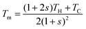 | (7) |
Tm has the unit of temperature. It is affected by the ratio
s and the hot and cold side temperatures.
Eqn (6) indicates that the heat flow through a thermoelectric generator will change with the ratio
s (by changing the external load resistance) if the temperature difference across the thermoelectric generator remains unchanged, or if the heat flow is kept constant, the temperature difference across the thermoelectric generator will change with the ratio
s. The term
ZTm in the equation represents the contribution of the Peltier heat to the total heat flow through the thermoelectric generator, in which
Z is the property of the thermoelectric generator and
Tm is associated with the operating condition, which is a function of
TH,
TC and
s.
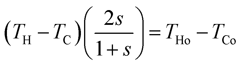
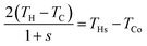
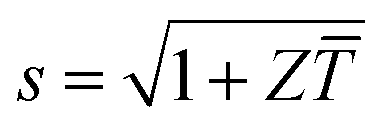
For a thermoelectric generator operating under a constant heat flux and assuming no heat loss from the system, the heat flux through the thermoelectric generator will remain the same for the open circuit and closed circuit (i.e., o = c). As a result, a relationship between ΔT and ΔTo can be established as
Eqn (8) indicates that the temperature difference across a thermoelectric generator will be reduced by a factor of (1 +
ZTm) as the circuit changes from open circuit to closed circuit.
Fig. 2 shows the temperature difference across a thermoelectric generator as a function of
s for different
Z values. It can be seen that the temperature difference across a thermoelectric generator decreases with
s, reaching a minimum value of Δ
Ts in a short circuit (
i.e.,
s = 0) and Δ
Ts becomes smaller with the increasing
Z. This is due to the fact that under a constant heat flux, the contribution to the heat flow due to the Fourier heat decreases while the contribution due to the Peltier heat increases with the increasing current as a result of reducing the external load resistance.
Eqn (8) reveals an inevitable consequence of the Peltier effect on thermoelectric power generation. Using this relation, it is possible to determine the actual temperature difference across a thermoelectric generator for a given material (
Z) and operating conditions (
s and Δ
To). This relation plays an important role in developing the theory of thermoelectric generators operating under a constant heat flux and lays the foundation for a deep understanding of the thermoelectric behaviour discussed below.
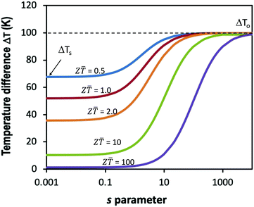 |
| | Fig. 2 Temperature difference across a thermoelectric generator as a function of ratio s for operation under constant heat flux. It is assumed that the cold side temperature of the thermoelectric generator is maintained at 300 K and the hot side temperature in the open circuit is 400 K. Z is the thermoelectric figure-of-merit ranging from 0.5 to 100. | |
4. Thermoelectric I–V curves
The I–V curve is a useful plot for many electronic devices (e.g., diodes and transistors), which reveals the key characteristics of the devices.12 The I–V curve is also extensively employed for determining the performance of solar cells.13 However, the I–V curves appear to have very limited application in thermoelectrics, which are mainly used to determine the power output of generators and in some cases were applied inappropriately leading to incorrect results. This is due to the fact that the thermal behaviour of a thermoelectric generator can be affected by I–V measurements due to the Peltier effect and in turn, it changes the profile of the I–V curve. Using eqn (8), this problem can now be understood, and correct applications can be formulated.
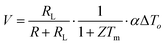
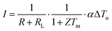
Based on the equivalent circuit of the thermoelectric generator shown in Fig. 1(b), the voltage across the load and the current flowing through the circuit can be expressed as
| | 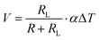 | (9) |
| |  | (10) |
For a thermoelectric generator operating under a constant temperature difference, Δ
To, its Seebeck coefficient,
α, and internal resistance,
R, will remain unchanged when changing the load resistance,
RL. A linear relationship between
V and
I is obtained as
However, if the thermoelectric generator operates under constant heat flux, a change in the load resistance,
RL, will result in a change in the temperature difference across the generator, which is governed by
eqn (8). In this case, the voltage and current can be expressed as
| |  | (12) |
| |  | (13) |
The relationship between
V and
I is given by
| | 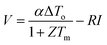 | (14) |
It can be observed that
eqn (14) shows approximately a linear relationship between
V and
I if
Z and Δ
To are not too large. For example, the coefficient of determination (a measure of linearity) is 0.9993 for a generator with
Z = 1 operating under Δ
To = 100 K, while it is 0.94797 for a generator with
Z = 10 operating under Δ
To = 1000 K (an example of the extreme case), indicating the validity of linear relationship in most cases.
The term that represents the open circuit voltage (αΔTo) in eqn (11) is reduced by a factor of (1 +ZTm) in eqn (14). This indicates that the thermoelectric I–V curve will be affected by the thermal response of a thermoelectric generator and consequently affected by the sweep rate of the I–V tracer. Fig. 3 shows the I–V curves obtained by fast and slow sweep rates, respectively, for a thermoelectric generator with Z = 1 operating under ΔTo = 100 K. Since the electrical response of a thermoelectric generator is at least an order of magnitude faster than the thermal response due to a large thermal inertia, the I–V curves obtained using a fast sweep rate (less than one second) is almost the same as if the thermoelectric generator operates under a constant temperature difference, which is governed by eqn (11) (blue line in Fig. 3). However, if a very slow sweep rate (e.g., 30 min per point) is used, the thermoelectric generator has an opportunity to reach the respective thermal steady-states corresponding to each of the set values of the load resistance, RL. As a result, a different I–V curve is obtained which is governed by eqn (14) (red line in Fig. 3).
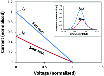 |
| | Fig. 3 Thermoelectric I–V curves for operating under a constant temperature difference (fast scan) and constant heat flux (slow scan), respectively. The inset shows the corresponding power outputs. | |
Since the slope of the I–V curve using a fast sweep rate is bigger than that using a slow sweep rate, the power output obtained from a fast sweep rate is significantly larger than that using a slow sweep rate as shown by the inset of Fig. 3. In essence, the maximum power output determined from an I–V curve of fast sweeping represents the case when a thermoelectric generator operates under a constant temperature difference (ΔT = 100 K in this example). However, due to the slow thermal response, the thermoelectric generator is unable to reach the corresponding thermal steady-state within the same timescale of I–V tracing. The heat flow through the thermoelectric generator determined in this way is equal to o (=KΔTo), not the corresponding thermal state c (=(1 + ZTm)KΔTo). As a result, the conversion efficiency determined in this manner is significantly overestimated. In order to obtain correct measurements, the thermoelectric generator needs to be connected to a matching load and wait until the thermal steady-state has been reached while maintaining the temperature difference across the thermoelectric generator constant. An alternative approach is to use the I–V curves of slow sweeping described below.
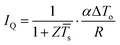
The I–V curves obtained from slow sweeping represent the case when a thermoelectric generator operates under constant heat flux. In this process, each set of the I–V data is measured after the thermoelectric generator has reached the corresponding steady-states. The maximum power output determined from this I–V curve corresponds to actual heat flow through the thermoelectric generator, which is also the heat flow under initial conditions because of the operation under a constant heat flow. Consequently, the conversion efficiency of the thermoelectric generator can be calculated directly using Pmax/Qo if slow sweeping is used. However, it is to be noted that the temperature difference across the thermoelectric generator in this case is smaller than ΔTo because the temperature difference will decrease in a closed circuit.
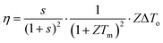
The open circuit voltage and short circuit current are the two characteristic parameters of the I–V curves. For a thermoelectric generator under given conditions, the open circuit voltage, Vo, is always the same regardless of whether the I–V curve is obtained by a fast or slow sweep. However, the short-circuit currents are significantly different for operation under a constant temperature difference and constant heat flux, which can be determined using eqn (10) and (13), respectively,
| |  | (15) |
| |  | (16) |
where
s = (
THs +
TC)/2 is the average temperature of the thermoelectric generator when the generator has reached a thermal steady-state corresponding to the electrical short circuit.
THs is the hot side temperature of the thermoelectric generator at the short circuit.
It is interesting to note that the good linearity of the I–V curves of thermoelectric generators is a crucial requirement for developing a novel measurement technique (see Section 6.3) but can also be viewed as a drawback. Using the definition of the “fill factor” of solar cells,13 one can determine the fill factor of thermoelectric generators, which is approximately 0.25 for all thermoelectric generators due to the straight line of their I–V curves. This value is less than 1/3 of the fill factor of typical solar cells. Furthermore, the thermoelectric fill factor is a constant that cannot be further increased if the I–V curves remain in a straight line. For the same open-circuit voltage and short-circuit current, the maximum power output produced by the thermoelectric process is significantly lower than that produced by the photovoltaic process. This raises the question if the thermoelectric process is inherently less efficient than the photovoltaic process, is there any thermoelectric process that produces an I–V curve similar to that of a photovoltaic device?
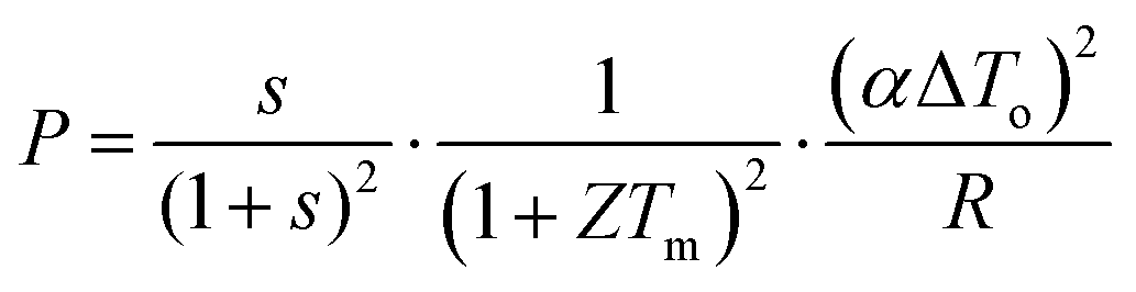
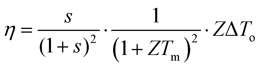
5. Power output and conversion efficiency
The performance of thermoelectric generators is evaluated by their power output and conversion efficiency. Using eqn (8), the theoretical procedure to calculate the power output and conversion efficiency of a thermoelectric generator that operates under constant heat flux can now be developed. Together with eqn (5), (12) and (13), the power output (P = I·V) and conversion efficiency (η = P/o) of a thermoelectric generator can be expressed as| | 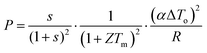 | (17) |
| |  | (18) |
In general, the temperature difference across the thermoelectric generator in an open-circuit (ΔTo) can be determined from the given heat input (o) and the thermal conductance of the thermoelectric generator (K) using eqn (5). If s and Tm are known, the P and η of the thermoelectric generator can be calculated using eqn (17) and (18). However, in most practical applications, we only need to determine the maximum power output, Pmax, and maximum conversion efficiency, ηmax. To achieve this, attempts were made to derive analytical expressions similar to eqn (3) and (4). However, it appears that there are no simple analytical solutions available for Pmax and ηmax in the case of constant heat flux and consequently, a numerical method has to be employed.
5.1 Numerical method (accurate approach)
The numerical method involves initially determining a set of s and Tm, followed by calculating all the corresponding values for P and η using eqn (17) and (18), and then identifying the Pmax and ηmax numerically or graphically. In order to determine Tm for a given s using eqn (7), we need to determine the hot side temperature of the thermoelectric generator, which can be done by rewriting eqn (8) as| | 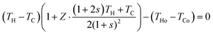 | (19) |
In the design of thermoelectric generators, the materials property (Z) and initial operating temperatures (THo and TCo) are usually known. In addition, it is a general practice to maintain the temperature at the cold side of the thermoelectric generator constant, i.e., TC = TCo. In this case, the corresponding value to a given s can be determined by finding the positive solution to eqn (19) and the corresponding Tm can be calculated using eqn (7). Table 1 lists the calculated Tm for a set of s parameters, together with TH and η. The data were calculated by assuming that THo = 400 K, TCo = 300 K and Z = 1. Using modern computational software such as MATLAB, the whole procedure can be programed and large sets of data can be calculated automatically. Fig. 4 shows the calculated conversion efficiency as a function of s for different Z values. Using this graph, the maximum efficiency and the corresponding optimal s can be determined. For example, in the case of Z = 1, the maximum conversion efficiency of 0.0351 is obtained at s = 1.9 (optimal s). Since the power output depends on s and Tm in the same manner as the conversion efficiency (see eqn (17) and (18)), the maximum power output is also obtained at the same optimal s. This differs from the operation under a constant temperature difference, where the maximum power output is obtained at s = 1 and the maximum conversion efficiency is obtained at  .
.
Table 1 Selected data of calculated TH, Tm and η for given s using the numerical procedure described. The data were calculated by assuming THo = 400 K, TCo = 300 K, and Z = 1. The calculation was performed using MATLAB
|
s
|
0.001 |
0.01 |
0.1 |
1 |
1.9 |
5 |
10 |
100 |
1000 |
|
T
H
|
351.78 |
351.98 |
353.87 |
366.65 |
373.74 |
384.74 |
390.86 |
398.88 |
399.91 |
|
T
m
|
325.59 |
323.02 |
299.44 |
174.99 |
124.49 |
62.947 |
35.157 |
3.9445 |
0.3995 |
|
η
|
0.0001 |
0.0008 |
0.0069 |
0.0318 |
0.0351 |
0.0285 |
0.0195 |
0.0027 |
0.0003 |
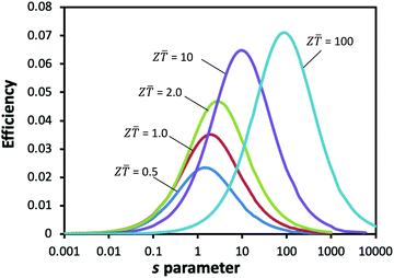 |
| | Fig. 4 The conversion efficiency of the thermoelectric generator as a function of s parameter for different Z values. The optimal values of s parameter to obtain the maximum conversion efficiency can be determined graphically. The temperature at the hot and cold sides of the thermoelectric generator in the open-circuit is assumed to be 400 K and 300 K, respectively. | |
Compared to the analytical approach, the numerical method appears to be more complex. However, with modern computing, the calculation can be performed quickly and conveniently once the code is written. The only drawback is the lack of direct physical intuition. The results can be better understood with reference to Fig. 2. When a thermoelectric generator operates under constant heat flux, the temperature difference across the generator varies with s (by changing the external load resistance, RL). In order to generate a large voltage, the temperature difference across the thermoelectric generator should be large, which corresponds to requesting a large s value. On the other hand, in order to produce a large current, a small s value is required which results in a smaller temperature difference. As a result, the maximum power output (also maximum conversion efficiency) is achieved by optimising the temperature difference across the thermoelectric generator through trade-off between the voltage and current. It can be seen from Table 1 that the hot side temperature at the optimal point is 373.74 K for Z = 1, which is approximately the middle point between the open-circuit (400 K) and short-circuit (351 K). Clearly, the optimisation process is very different from the operation under the constant temperature difference, where the optimisation is a trade-off between the power output and heat flux.
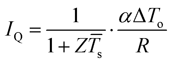
5.2 Analytical method (approximate approach)
Although the accurate calculation of Pmax and ηmax is only possible using the numerical method, an approximate analytical approach can be developed based on the linear relation between the voltage and current of thermoelectric generators. For a device with a perfect linear I–V characteristic, its maximum power output is always obtained at the middle point of the I–V curve (i.e., corresponding to Vo/2 and IQ/2) as shown in Fig. 5. In this case, an equation can be derived based on the condition V = Vo/2 using eqn (8), (12) and Vo = αΔTo,| |  | (20) |
In most power generation applications, THo and TCo are usually given and the Z value is known. In addition, the cold side of the thermoelectric generator can be maintained constant, i.e., TC = TCo. In this case, an optimal sV and the corresponding TH can be determined by simultaneously solving eqn (19) and (20). Then, the maximum power output and maximum conversion efficiency can be calculated using eqn (17) and (18).
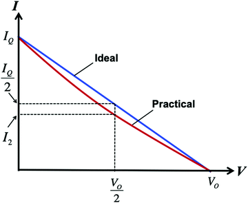 |
| | Fig. 5 Schematic thermoelectric I–V curves. The blue-line represents an ideal I–V curve that is a perfect straight line. The red-line represents a practical I–V curve that is slightly curved. In the ideal case (blue), the middle point on the voltage axis corresponds to the middle point on the current axis because of the perfect straight line. In the practical case (red), the middle point on the voltage axis no longer corresponds to the middle point on the voltage axis. | |
It is to be noted that the calculation procedure described above is only valid for a perfectly linear I–V curve. As mentioned earlier in Section 4, the thermoelectric I–V curves are, in general, only approximately linear. As a result, an error will occur due to non-linearity as shown in Fig. 5. However, it is found that the accuracy of this method can be significantly improved by using an averaging procedure. Similar to using the condition V = Vo/2, we can also use the condition I = IQ/2. Based on this condition, together with eqn (13) and (16), an equation can be derived as follows
| |  | (21) |
where
THs is the hot side temperature of the thermoelectric generator in the short-circuit, which is usually unknown but can be calculated by solving the equation below
| |  | (22) |
Eqn (22) is a special case of
eqn (19) in the short circuit (
i.e., when
s = 0). Once
THs is determined using
eqn (22), an optimal
sI and corresponding
TH can be determined by solving
eqn (19) and (21) simultaneously. Then, an average optimal value can be obtained by
![[s with combining macron]](https://www.rsc.org/images/entities/i_char_0073_0304.gif)
= (
sV +
sI)/2.
Fig. 6 shows the maximum conversion efficiency and the hot side temperature as a function of the thermoelectric figure-of-merit,
Z, for a thermoelectric generator operating under a constant heat flux with its initial open-circuit temperature difference of Δ
To = 100 K (
i.e.,
THo = 400 K and
TCo = 300 K). The data were calculated using the approximate method described above. For a thermoelectric generator with
Z = 1, the calculated
ηmax and
TH are 0.03514 and 373.9 K, respectively, which shows an excellent agreement with the results from the numerical method as shown in
Table 1. It can be shown that the deviation in the maximum conversion efficiency between the numerical method and the approximate method is typically less than 2% even for the extreme case scenario of
Z = 10 and Δ
To = 1000 K. Using the analytical method, the computational requirement for determining the maximum conversion efficiency is significantly reduced without noticeable compromise in accuracy.
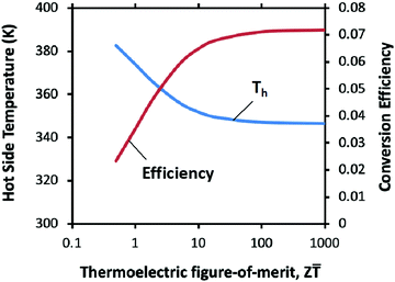 |
| | Fig. 6 The maximum conversion efficiency and corresponding hot side temperature as a function of thermoelectric figure-of-merit, Z, for a thermoelectric generator operating under a constant heat flux with its initial open-circuit temperature difference of ΔTo = 100 K (i.e., THo= 400 K and TCo = 300 K). The efficiency improvement beyond Z > 10 is less significant. | |
6. Potential applications
The new formulation provides a theoretical tool for the design, optimisation and evaluation of thermoelectric generators that operate under constant heat flux. Moreover, it offers a new perspective on investigating the response of thermoelectric generators when operating under constant heat flux and lays the foundation for potential new applications. As can be seen from the discussion above, the characteristics of heat sources have a profound influence on the operation of thermoelectric generators. An appropriate design and application of thermoelectric generators require good knowledge and understanding of the characteristics of heat sources.
6.1 Heat sources
The characteristics of heat sources have a significant impact on the design and performances of thermoelectric generators that have frequently been overlooked. An initial step in the design of thermoelectric generators should identify the characteristics of heat sources. In general, heat sources can be divided into a “constant-temperature” heat source and a “constant-flux” heat source (similar to the concept of the constant voltage source and constant current source). An ideal constant-temperature heat source has the ability to maintain the temperature of the heat source unchanged while the heat flux varies with the thermal conductance of a thermal load. On the other hand, an ideal constant-flux heat source has the ability to maintain the heat flux unchanged while its temperature can vary. In the real world, it is likely that both the temperature and heat flux of a heat source will change. However, in most cases, either the temperature of a heat source changes much quickly than the heat flux or vice versa, enabling approximation to one type or the other. For example, the hot water circulating through a heat exchanger can be approximated as a constant-temperature heat source. The hot water carries a large amount of thermal energy due to its high specific heat capacity and continuous water circulation. This allows the heat flux to vary without significantly affecting its temperature. On the other hand, a solar thermal absorber can be viewed as a constant-flux heat source. The amount of thermal energy collected by the absorber is fixed. If radiative heat loss is negligible, the heat flux through a thermal load will be equal to the absorbed energy and hence remains constant, while the temperature is likely to change with the thermal conductance of a thermal load (another similar case is the radioisotope heat source, which has been employed in thermoelectric space power systems). An implication for real-life application is that heat losses due to heat convection and radiation will also change with the thermal load when operating under constant heat flux. However, the new formulation will be valid if the heat flux through the thermoelectric generator is kept constant.
The thermal energy extracted from hot fluid such as vehicle exhaust is an interesting case that can change from one type to another. The thermal energy is extracted through a heat exchanger and the effectiveness of the heat exchanger determines the characteristics of the heat source. If the heat exchanger extracts thermal energy at a rate that is significantly higher than the heat flux required by a thermal load, it behaves like a constant-temperature heat source. Otherwise, it will be a constant-flux heat source. In general, when a steady state is reached between the heat source and its thermal load, we have H = G + L (where H is the rate of heat production by a heat source, G is the heat flux through a thermal load and L is the rate of heat losses). If G ≪ H, the system is likely to operate in a constant temperature mode. If G ≈ H, the system is likely to operate in a constant heat flux mode. Clearly, for efficient use of thermal energy, a thermoelectric generator should be designed to operate in a constant heat flux mode.
6.2 Design and optimisation
The new formulation is developed to assist the evaluation of the performance of thermoelectric generators for design and optimisation. Fig. 7 shows the maximum conversion efficiency of a thermoelectric generator as a function of Z for different operating temperatures. Fig. 7(a) is calculated using the new formulation, which represents the situations when the thermoelectric generator operates under constant heat flux. Fig. 7(b) is calculated using the established theory, which represents the situations when the thermoelectric generator operates under a constant temperature difference. Comparing Fig. 7(a) with (b), it appears that a thermoelectric generator that operates under a constant temperature difference is much more efficient than that under constant heat flux. However, such a comparison is flawed because these two operating modes are not directly comparable. Although the initial temperature differences (ΔTo) across a thermoelectric generator are the same for both operating modes, the actual temperature differences (ΔT) across the thermoelectric generator when operating at their respective maximum efficiency points are considerably different. In the case of constant temperature difference, the temperature difference corresponding to its maximum efficiency point is the same as that in an open circuit (i.e., ΔT = ΔTo). However, it is considerably lower in the case of constant heat flux (i.e., ΔT ≪ ΔTo) as shown in Table 2. This is due to the fact that different types of heat sources react to the occurrence of the Peltier effect differently. In an open circuit, there is no electrical current flowing through the thermoelectric generator and hence no Peltier heat. However, the Peltier heat will appear when the thermoelectric generator is in a closed circuit. Since the heat flux cannot change when operating under a constant heat flux, the presence of the Peltier heat must be accompanied by a decrease in the Fourier heat, which leads to a reduction in the temperature difference across the thermoelectric generator. This is very different from the case of operation under a constant temperature difference, where the Peltier heat is topped up by the heat source while the Fourier heat remains constant and consequently, the temperature difference remains unchanged. Clearly, the comparison between these two cases becomes irrelevant because both the temperature difference and heat flux are very different when they reach their respective maximum efficiency points, even though the temperature difference and heat flux for both cases are exactly the same in open circuits.
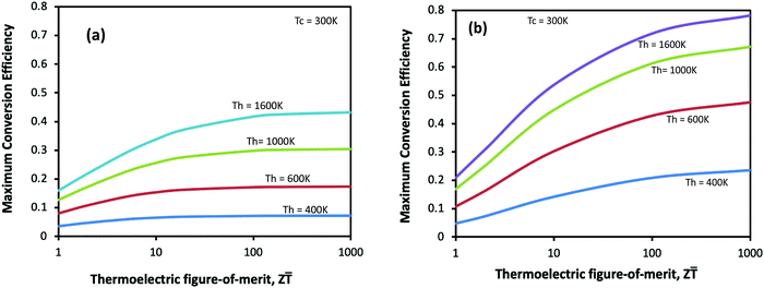 |
| | Fig. 7 The maximum conversion efficiency as a function of Z for different operating temperatures. (a) The data were calculated using the new theory developed in this work, which assumes that the thermoelectric generator operates under a constant heat flux. (b) The data were calculated using the established theory, which assumes that the thermoelectric generator operates under a constant temperature difference. The efficiency improvement beyond Z > 10 is less significant in the case of operation under constant heat flux. | |
Table 2 The hot side temperatures and temperature differences across a thermoelectric generator in an open circuit (THo and ΔTo) and in a closed circuit (TH and ΔT) under a constant heat flux for the cold side temperature maintained at 300 K and the thermoelectric figure-of-merit of ZT = 1. The corresponding maximum conversion efficiency is also included
|
T
Ho (K) |
T
H (K) |
ΔTo (K) |
ΔT (K) |
η
max
|
| 400 |
373.9 |
100 |
73.9 |
0.0351 |
| 600 |
518.3 |
300 |
218.3 |
0.0804 |
| 1000 |
802.1 |
700 |
502.1 |
0.1277 |
| 1600 |
1224.4 |
1300 |
924.4 |
0.1606 |
Let us consider an extreme case that may never be achievable in practice but has an important theoretical significance. The condition and implication of a thermoelectric generator to approach the ultimate limit of the conversion efficiency are different for these two cases. Eqn (4) indicates that the maximum efficiency of a thermoelectric generator that operates under a constant temperature difference is able to approach the Carnot efficiency if the Z value approaches infinity. However, there is a hidden factor in this equation. In order to reach the Carnot efficiency, it requires Z to approach infinity while maintaining the temperature difference unchanged. This, in turn, requires the heat flux through the thermoelectric generator to approach infinity as indicated by eqn (6). Obviously, this is impossible in practice. Towards this ultimate limit, eqn (4) predicts the best prospect that is only attainable in principle, but it is unlikely to be achievable in practice. On the other hand, the new formulation is built on an assumption that the input heat power is fixed. The process does not involve unreasonable requirements and hence the ultimate limit of the conversion efficiency predicted using this new formulation is more attainable realistically. In order to change from an open circuit to a maximum power point when operating under a constant temperature, a thermoelectric generator has to obtain a significant amount of extra energy from the heat source to increase the heat flux while maintaining a constant temperature difference. When operating under constant heat flux, on the other hand, the thermoelectric generator does not require any top-up of energy input from the heat source. Instead, the transition from an open circuit to the maximum power point state is achieved by reducing its temperature difference across the hot and cold sides.
It is intriguing to note that although the conversion efficiency appears to be higher under a constant temperature difference, it could be more efficient by designing a thermoelectric generator under constant heat flux. This argument can be understood by considering an imaginary case where a thermoelectric generator is driven by an “ideal heat source” that can change from a constant temperature mode to a constant heat flux mode. Assuming that the thermoelectric generator operates initially under a constant temperature difference (ΔTo1), when reaching the maximum efficiency point, the heat flux through the thermoelectric generator will be increased due to the appearance of the Peltier heat, which is topped up by the heat source. The total heat flux in this case can be calculated using eqn (6). Imagine that the heat source is now changed to the constant heat flux mode and the thermoelectric generator returns to the open circuit, its temperature difference will increase to ΔTo2, which will be larger than ΔTo1. It can be shown that when the thermoelectric generator makes the transition from an open circuit to the maximum power point based on ΔTo2 under a constant heat flux mode, the conversion efficiency of the thermoelectric generator is slightly higher than that based on the “equivalent” constant temperature difference mode because the optimal s is different for these two cases.
Another important implication of the new formulation in the design of a thermoelectric generator can be seen in Table 2. If a thermoelectric generator is driven by a heat source of constant heat flux, the hot side temperature of the thermoelectric generator at the maximum conversion efficiency point (TH) is much lower than that in the open circuit (THo). This behaviour could lead to potential damage to a thermoelectric generator if designers are not aware of this behaviour. For example, if a thermoelectric generator is designed to operate at 802 K with a matched load to obtain the maximum efficiency, its hot side temperature will increase to 1000 K if the load is disconnected from the thermoelectric generator, leading to overheating and consequently, damage to the hot side of the thermoelectric generator (see Table 2).
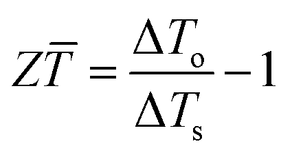
6.3 New ZT measurement method
Considering the two special cases of operation in the open circuit (RL = ∞) and short circuit (RL = 0), eqn (8) can be rearranged as,| |  | (23) |
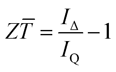
This indicates that the thermoelectric figure-of-merit, Z, can be determined by measuring the temperature differences ΔTo and ΔTs, respectively. Furthermore, an equivalent relationship can be derived from eqn (15) and (16),14| |  | (24) |
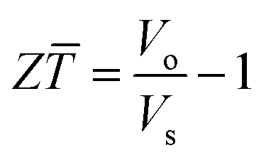
Eqn (24) indicates that Z can also be determined if IΔ and IQ are known. The advantage of using eqn (24) is that IΔ and IQ can be conveniently determined from the I–V curves shown in Fig. 8, where IΔ is the intercept on the I-axis of the I–V curve obtained using a fast sweep rate and IQ is the intercept on the I-axis of the I–V curve obtained using a slow sweep rate. However, eqn (24) is derived based on an assumption that the resistance of thermoelectric materials remains unchanged. This is usually valid if the temperature difference across the thermoelectric device is small (<50 K). If the temperature difference is large, this assumption is no longer valid. In this case, a third I–V curve can be acquired by another fast sweep once the IQ is reached after the slow sweep of the second I–V curve. As shown in Fig. 8, the voltage corresponding to the open-circuit, Vo, and the short-circuit, Vs, can be determined from these I–V curves and the thermoelectric figure-of-merit, Z, can be determined using,| |  | (25) |
Eqn (25) does not require the above assumption and is valid even if the resistance changes. The accuracy of this measurement method relies on the ability to meet two conditions: (1) maintaining a constant thermal input and (2) achieving a short circuit. These requirements can be easily met using a thermoelectric module because of the favourable geometry and large internal resistance. However, it becomes very challenging when it is used to characterise a single piece of thermoelectric material due to the conflicting requirements on the sample geometry to achieve large resistance and minimum heat loss of the sample.
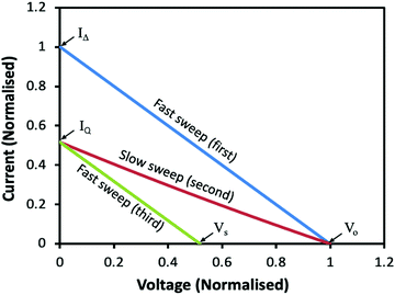 |
| | Fig. 8
I–V curves of a thermoelectric generator obtained by (a) fast sweep (blue), (b) slow sweep (red) and (c) fast sweep starting from IQ (green). | |
The dimensionless thermoelectric figure-of-merit, Z, is the most important parameter in thermoelectric research, which determines the conversion efficiency of thermoelectric devices (generator or refrigerator) under a given operating condition. Several measurement techniques are already available.15 However, all current techniques can only measure Z under a small temperature difference (usually < 20 K). A unique aspect of this method is the capability of Z measurement under a large temperature difference. This feature offers the possibility for the characterisation of complex thermoelectric structures such as segmented and functionally graded materials. In addition, it enables the study of the impact of other transport phenomena that only become significant under large temperature difference, such as the Thompson effect (which only exists when there is an electrical current flowing through the material and becomes significant under a large temperature difference). The development of this technique can have a profound impact on thermoelectric technology.
6.4 Variable thermal resistance
The ability to control heat flow between two thermal bodies has useful applications in thermal engineering. This requires the ability to change the thermal conductance of the material between two thermal bodies. Eqn (6) provides the underlying principle for such a possibility by using thermoelectric materials. Based on eqn (6), we can define the effective thermal conductance of a thermoelectric material asIt can be seen from eqn (7) that ZTm can vary between 0 and Z by changing the external electrical resistance, RL. Currently, the Z value for commercially available materials is approximately 1. This indicates that the technology is already available to develop variable thermal resistance that has the capability to regulate heat conduction by a factor of 2. The range of variation can be further increased if high Z materials can be developed in the future. The advantage of this method is that the variation of thermal resistance is controlled by changing the electrical resistance of an external resistor, which can be achieved conveniently. Although the change of effective thermal conductance is associated with the Peltier heat, no external electrical power is needed because the Peltier heat in this case is produced by the self-generated electrical current when the thermoelectric material is subjected to a temperature difference.
6.5 Pulse mode operation
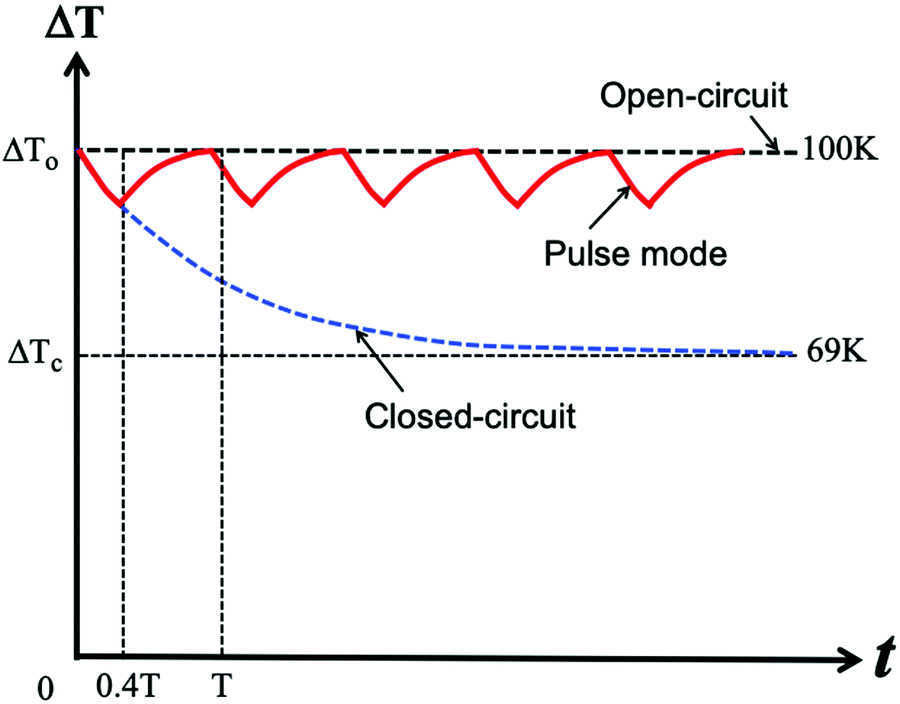
The Kelvin relation describes the fundamental connection between the Seebeck effect and the Peltier effect. The advantages and benefits of this relation are well known.1–4 However, the Kelvin relation also imposes an adverse influence on the performance of thermoelectric generators. Due to the Peltier effect, the temperature difference across a thermoelectric generator in a closed circuit will be reduced and consequently, a decrease in the power output. The larger the Z value, the more significant the reduction (see Fig. 2). Clearly, minimising the influence of the Peltier effect during thermoelectric generation would help to improve the performance of a thermoelectric generator. A possible way is to operate the thermoelectric generator in a pulsed mode. The essence of the idea lies in the exploitation of the different response rates of electrical and thermal processes, which can be explained in Fig. 9. For a thermoelectric generator operating in a continuous mode with the matched load (in order to deliver the maximum efficiency), the temperature difference across the thermoelectric generator will be reduced from original ΔTo = 100 K to ΔT = 74 K when reaching the steady state. This will result in a significant reduction in the power output because the power is proportional to the square of the temperature difference. However, the temperature difference across a thermoelectric generator could be maintained in the vicinity of the original ΔTo by the pulse mode operation, in which a small drop in temperature during the switch-on period can be compensated by the increase during the switch-off period as shown in Fig. 9. Although there will be heat loss during switch-off, it is possible that the power generated during the switch-on period under a large temperature difference can over-compensate the loss due to a small temperature difference in the continuous mode. Such a possibility has been demonstrated based on quantitative analysis using eqn (8).14 The results indicate that the benefit is not significant unless the Z value becomes large. This is due to the fact that the significant reduction in temperature difference occurs at large Z and the heat loss during the switch-off period is relatively small compared to the Peltier heat.
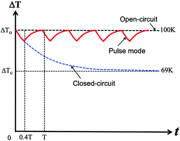 |
| | Fig. 9 Schematic temperature profile of a thermoelectric generator operating under constant heat flux in two different modes. The dashed line (blue) shows the temperature profile when operating under a steady state. The solid line (red) represents the temperature profile when the generator operates in a pulsed mode. | |
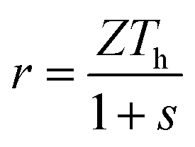
When a thermoelectric generator operates at its maximum efficiency point, the heat flux through the thermoelectric generator consists mainly of the Peltier heat and the Fourier heat (the Joule heat is usually much smaller compared to the above two). The ratio of the Peltier heat to the Fourier heat can be expressed as
| |  | (27) |
Table 3 shows the dependence of the ratio,
r, on the thermoelectric figure-of-merit,
Z, for a thermoelectric generator operates at its maximum efficiency point under the initial temperature of Δ
To = 100 K. It can be seen from
Table 3 that the hot side temperature,
Th, decreases while
r increases with the increasing
Z, indicating that the benefit of the pulse mode operation is more significant for thermoelectric generators with a large
Z. This conclusion might not have a direct practical benefit at the moment; however, it provides proof of principle that the adverse influence of the Peltier effect on a thermoelectric generator can be “decoupled”.
Table 3 The ratio of the Peltier heat to the Fourier heat, r, listed against the thermoelectric figure-of-merit, Z, for the generator operating at its maximum conversion efficiency point. The data were calculated assuming that the temperature difference in an open-circuit temperature is ΔTo = 100 K and the cold side temperature of the generator remains constant at 300 K
|
Z
|
1 |
2 |
5 |
10 |
100 |
1000 |
|
Z
|
0.00286 |
0.00571 |
0.01429 |
0.02857 |
0.28571 |
2.85714 |
|
s
|
1.935 |
2.823 |
5.453 |
9.800 |
87.87 |
868.5 |
|
T
h
|
373.9 |
365.2 |
356.1 |
351.8 |
347.0 |
346.5 |
|
r
|
0.364 |
0.545 |
0.789 |
0.930 |
1.116 |
1.139 |
7. Conclusions
The new formulation described in this work provides a theoretical framework for calculating the power output and conversion efficiency of thermoelectric generators that operate under constant heat flux. It expanded the capability of the current theory of thermoelectric generators to the point of completion, where the behaviour and performance of thermoelectric generators operating under a constant temperature difference and under constant heat flux can now be understood and evaluated. A numerical procedure has been established for the accurate calculation of the performance of thermoelectric generators. An approximate analytical method has also been developed to reduce the computing time, which is found to be in good agreement with the numerical method.
The new formulation provides important insights into the unique characteristics of thermoelectric generators when operating under constant heat flux. The most distinctive aspect is that the hot side temperature of the thermoelectric generator will change with the electrical resistance of the load, resulting in a more complicated optimisation procedure. An important implication of this work is that an initial and important step in thermoelectric generator design is to assess the characteristics of heat sources in order to achieve appropriate design. The result of efficiency analysis shows that the performance predicted based on the case of constant temperature difference represents the most promising scenario while the performance predicted based on the case of constant heat flux represents the realistic possibility.
Eqn (8) describes a thermoelectric relationship that links the temperature difference across a thermoelectric generator in a closed circuit to that in an open circuit. In addition to an important role played in formulating the new theory of thermoelectric generators, it also enables incorporating the thermal process into electrical I–V curves, leading to the possibility of I–V representation of thermoelectric processes. In addition, eqn (8) paves the way for some promising applications, including developing a new Z measurement technique and exploiting variable thermal resistance for heat flow control. Furthermore, radical concepts, such as minimizing the adverse Peltier effect by pulse mode operation or searching for non-linear I–V thermoelectric phenomena, are discussed.
Conflicts of interest
There are no conflicts to declare.
Acknowledgements
This work is partially supported by the EU RFCS programme through the InTEGrated project (899248) and partially supported by the EPSRC (UK) project (EP/K029142/1).
References
-
A. F. Ioffe, Semiconductor Thermoelements and Thermoelectric Cooling, Infosearch, London, 1957 Search PubMed.
-
D. M. Rowe and C. M. Bhandari, Modern Thermoelectrics, Holt, Rinehart and Winston, London, 1983 Search PubMed.
-
D. M. Rowe, CRC Handbook of Thermoelectric, CRC Press, Boca Raton, FL, 1995 Search PubMed.
-
D. M. Rowe, CRC Handbook of Thermoelectrics: Micro to Nano, CRC Press, Boca Raton, FL, 2005, ch. 11 Search PubMed.
- Lon E Bell, Cooling, Heating, Generating Power, and Recovering Waste Heat with Thermoelectric Systems, Science, 2008, 321, 1457–1461 CrossRef CAS PubMed.
- D. Champier,
Thermoelectric generators: A review of applications?, Energy Convers. Manage., 2017, 140, 167–181 CrossRef.
- G. Tan, M. Ohta and M. G. Kanatzidis, Thermoelectric power generation: from materials to devices, Philos. Trans. R. Soc., A, 2019, 377, 20180450 CrossRef CAS PubMed.
- N. Nandihalli, C. Liu and T. Mori, Polymer based thermoelectric nanocomposite materials and devices: Fabrication and characteristics, Nano Energy, 2020, 78, 105186 CrossRef CAS.
- G. Min and D. M. Rowe, A novel principle allowing rapid and accurate measurement of a dimensionless thermoelectric figure of merit, Meas. Sci. Technol., 2001, 12, 1261–1262 CrossRef CAS.
- G. Min, TE module theory for given thermal input, J. Electron. Mater., 2013, 42(7), 2239–2242 CrossRef CAS.
- G. Min and N. Md Yatim, Variable thermal resistor based on self-powered Peltier effect, J. Phys. D: Appl. Phys., 2008, 41, 222001 CrossRef.
-
M. J. Deen and F. Pascal, Springer Handbook of Electronic and Photonic Materials, ed. S. Kasap, P. Capper, Springer International Publishing AG, 2017 Search PubMed.
-
K. Mertens, Photovoltaics Fundamentals, Technology and Practice?, John Wiley & Sons Ltd, 2014 Search PubMed.
- G. Min, Principle of determining thermoelectric properties based on I–V curves, Meas. Sci. Technol., 2014, 25, 085009 CrossRef.
-
H. J. Goldsmid, Electronic Refrigeration, London, Pion, 1986 Search PubMed.
|
| This journal is © The Royal Society of Chemistry 2022 |
Click here to see how this site uses Cookies. View our privacy policy here. 
 Open Access Article
 This Open Access Article is licensed under a

 , respectively1


 .
.