
 Open Access Article
 This Open Access Article is licensed under a
 Creative Commons Attribution 3.0 Unported Licence
Atmospheric effects of air pollution during dry and wet periods in São Paulo†
Sergio
Ibarra-Espinosa
 a,
Gyrlene Aparecida
Mendes da Silva
b,
Amanda
Rehbein
a,
Angel
Vara-Vela
ac and
Edmilson
Dias de Freitas
a
a,
Gyrlene Aparecida
Mendes da Silva
b,
Amanda
Rehbein
a,
Angel
Vara-Vela
ac and
Edmilson
Dias de Freitas
a
aDepartamento de Ciências Atmosféricas, Instituto de Astronomia, Geofísica e Ciências Atmosféricas, Universidade de São Paulo, São Paulo-SP, Brazil. E-mail: zergioibarra@gmail.com
bInstituto do Mar, Universidade Federal de São Paulo, Santos-SP, Brazil
cFederal University of Technology - Parana, Londrina, Brazil
First published on 23rd December 2021
Abstract
Air pollutants reach high concentrations in developing countries, such as Brazil. The state of São Paulo is the economic and demographic center of Brazil and presents high levels of urbanization, fleet, and air pollution. Air pollutant concentrations are driven by meteorology, but aerosols present in polluted air also interact and change meteorological parameters due to their primary and secondary feedback effects. The objective of this study is to evaluate the impact of on-road transportation emissions on air pollutant concentrations and meteorology. Vehicular emissions were estimated using the VEIN model with a bottom-up fuel-calibration approach, and air pollutant concentrations were simulated using the WRF-Chem model considering dry and wet periods for Southeast Brazil. A 3 km grid spacing was considered for the inner domain to account for mesoscale circulation. Air pollutant simulations aligned with observations. Regarding the aerosol feedback, stronger interactions were found during the wet period. It was found that the effect of aerosols reduces 1.3% of downward solar radiation and 1.5% of O3, during the dry period. Furthermore, indirect effects of aerosols resulted in more precipitation, a higher planetary boundary layer, and lower levels of air pollutants in cities.
Environmental significanceAir pollution is an environmental problem, which affects the human health, ecosystems and the atmosphere. Aerosols affect the atmosphere by absorbing and scattering solar radiation and also the genesis and development of clouds. Road transportation is the main source of air pollution in megacities. This work presents a new vehicular emission inventory based on 124 million observations from smart-devices with GPS. The emissions are then input into an air quality model to model air pollutant concentrations. Lastly, this work evaluates the effects of aerosols during dry and rainy periods in South-east Brazil. |
1. Introduction
The evolution of air pollution is inherently related to meteorology.1 For instance, concentrations of nitrogen oxides (NOx) and volatile organic compounds (VOC) transported downwind generate ozone in the presence of solar radiation.2,3 Meteorology is also affected by air pollutant concentrations with feedbacks driven by interactions between solar radiation, aerosols and VOCs.4 Furthermore, aerosols have a direct radiative forcing effect by absorbing and scattering solar radiation and an indirect effect by increasing cloud condensation,5 thus altering radiative properties of cloud-precipitation.6,7 For example, several studies have found that aerosols impair solar radiation and surface temperature, and increase cloud droplets.8,9 Particulate matter (PM) is an important source of aerosols, largely emitted during biomass-burning, in urban and industrial areas, affecting the atmospheric circulation pattern.10 Therefore, it is important to enhance the understanding of interactions between air pollution and meteorology, especially in regions with limited environmental information, such as Latin America.Air pollution is a threat to human health with implications at global, regional, and local scales.11 As observed by Tsai et al.12 evidence shows that there is no adaption to prolonged exposure to PM10 levels (particulates with an aerodynamic diameter of less than 10 μm) over time; instead, there is a propagation of the inflammatory process. In December 2019, the Severe acute respiratory syndrome coronavirus 2 (SARS-CoV-2)13,14 was first reported in Hubei Province, China, and spread around the world. Its stability is on average 3 hours in aerosols, in addition to being potentially transported long to middle distances.15,16 Furthermore, transmissions made by aerosols have been highly underestimated, and now there is an active line of research.17–19 Also, high PM2.5 poses an additional risk of infection and deaths by COVID-19.20,21 Therefore, it is very important to study interactions between air pollutant concentrations and the physical–chemical aspects of the atmosphere, particularly, in developing countries such as Brazil.
Brazil is the biggest and most populated country in Latin America, with 8.510.295914 km2 of territorial area and an estimated population of 211.755.692 in 2020.22 The biggest cosmopolitan and financial region is located in Southeast Brazil and is formed by the agglomeration of São Paulo city and its surrounding areas that include coastal cities as well. These cities suffer high levels of air pollutants from anthropogenic activities, with on-road vehicles being the main source in metropolitan areas.23–25 The weather and climate of Southeast Brazil suffer the direct influence of meteorological systems from tropical, subtropical, and extratropical genesis,26,27 closely linked to low-frequency variability in interseason,28 interannual,29,30 and interdecadal31,32 timescales. Meteorological systems can promote the dispersion of air pollutants or trap them. For example, in the coastal part of this region, the concentrations can interact with mesoscale circulations, such as the sea breeze,33,34 increasing and transporting air pollutants from and to this region. Many air quality modelling studies conducted over Brazil have focused on the metropolitan areas of São Paulo.35–39 However, there are many remaining uncertainties about the role that urban emissions from large and mid-sized cities in Southeast Brazil play in air pollutant levels and meteorology changes in each one of these areas.
This study aims at investigating the relationships among emissions, meteorology, and air quality in Southeast Brazil. Therefore, we analyzed air quality conditions under different weather conditions in 2014, in order to answer the following questions: (i) how is the representation of air pollutant concentrations over dry and wet periods? (ii) What is the impact of aerosol effects on meteorology and air pollution during these periods? Then, we compiled a street-level vehicular emission inventory with activity data based on the Global Positioning System (GPS) using the Vehicular Emissions Inventories model (VEIN).25,40 Air quality simulations were conducted using the Weather Research and Forecasting (WRF) model coupled with Chemistry (WRF-Chem)41 in order to understand the impact of vehicular emissions on air quality and the impact of the total emissions on concentrations and their interactions with meteorology through aerosol feedbacks.
2. Materials and methods
2.1. Study area, periods and data
The study area is located in the domain of 47.94067° W to 45.38934° W and 24.57928° S to 22.41285° S, hereafter referred to as Southeast Brazil, as shown in Fig. 1. This study area covers the highly urbanized metropolitan areas of São Paulo, Santos, Campinas, São José dos Campos and Sorocaba cities, totalizing about 30 million inhabitants.22 The periods of study were determined firstly by selecting a dry and polluted period, found in October 2014, which was followed by a rainy period in November 2014. Then, wet (rain above 1 mm per day) and dry (rain less than 1 mm per day) periods were detected using the Integrated Multi-satellitE Retrievals for Global Precipitation Measurement (IMERG).42 In this sense, the dry period covers October 5th–10th, 2014, and the wet period covers October 31st–November 5th, 2014. The temporal evolution of air pollutant concentrations, such as carbon monoxide CO (ppm), nitrogen monoxide NO (μg m−3), nitrogen dioxide NO2 (μg m−3), particulate matter with an aerodynamical diameter lower than 10 micrometers, PM10, and lower than 2.5 micrometers, PM2.5 (μg m−3), and ozone, O3 (μg m−3), were analyzed using data from the São Paulo State Environmental Company (CETESB). CETESB also provides meteorological data such as temperature (°C), atmospheric pressure at the station level (hPa), wind speed (m s−1), and global solar radiation (W m−2). In the case of precipitation, the data were obtained from the National Institute of Meteorology (INMET). The description of the observation sites is available in Table S1 of the ESI†. | ||
| Fig. 1 Area of study including metropolitan areas of Campinas (CAM), São Paulo (MASP), Sorocaba (SOR), São José Dos Campos (SJDC) and Santos (SAN). This figure represents the inner domain for the numerical modeling and the grey box, at bottom left the coarser domain. Digital elevation map from ASTER/NASA Earth Data (https://earthdata.nasa.gov/). | ||
2.2. Atmospheric conditions
The synoptic analysis was initially made on a daily basis by identifying the weather patterns that impact the climate and weather over São Paulo and actuated each day through the synoptic charts, satellite images, and meteorological conditions at the surface, as shown in ESI Fig. S10, S11† for 00 UTC for brevity, and Fig. 2. The synoptic charts are from the Center for Weather Forecasting and Climate Studies (CPTEC; http://img0.cptec.inpe.br/%7Ergptimg/Produtos-Pagina/Carta-Sinotica/Analise/) for the surface, low, middle and upper levels and for the four synoptic available times (00 UTC, 06 UTC, 12 UTC, and 18 UTC); satellite images are from the Geostationary Environmental Satellite (GOES-13, http://satelite.cptec.inpe.br/acervo/goes.formulario.logic?i=en) infrared channel (∼11.0 μm); meteorological conditions such as 2 m air temperature, relative humidity, wind speed and direction, and solar radiation are from the INMET surface station (https://bdmep.inmet.gov.br/). We also compared the pollutant concentrations in both periods with the meteorological conditions using surface stations from INMET and CETESB.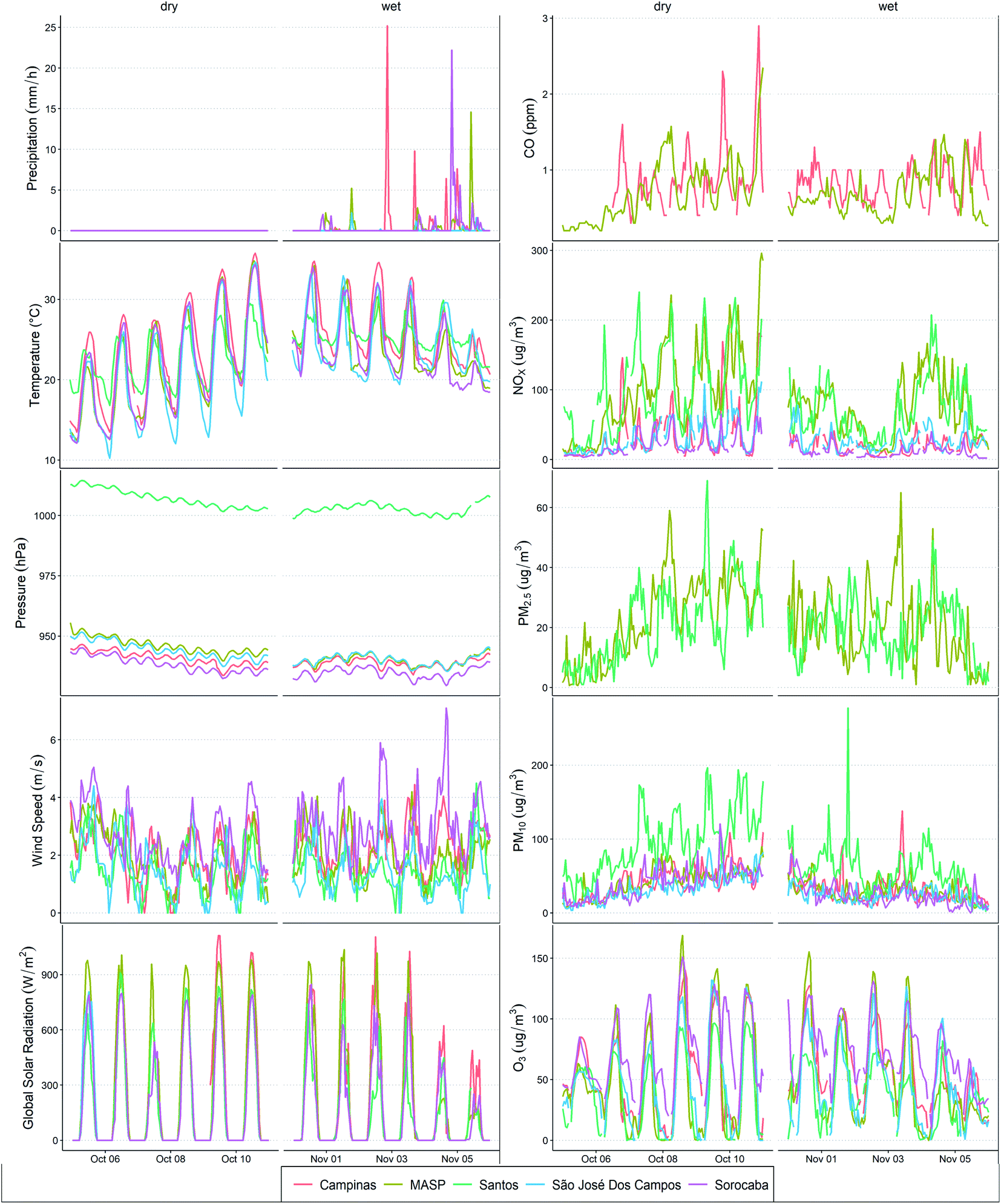 | ||
| Fig. 2 Hourly meteorological parameters (on the left) and air pollutant concentration (on the right) observations averaged by each metropolitan region for the dry (October 05th−10th, 2014) and wet (October 31st–November 05th, 2014) periods. Campinas was abbreviated as CAM, Santos as SAN, São José Dos Campos as SJDC, Sorocaba as SOR and the metropolitan area of São Paulo as MASP. Precipitation from INMET and other parameters from CETESB. | ||
2.3. Emissions inventory
Air pollutants are generated by chemical species released by sources to the atmosphere, which vary over time and region. In the study area, the most important source of air pollution is vehicles, except for the Santos city that is mainly impacted by industrial sources. The emission inventory covers on-road sources where traffic flows were derived from a massive dataset of GPS-enabled devices registered in October of 2014 in the study area.43 The traffic flows were generated for the morning rush hour and then extrapolated to 24 hours with hourly traffic counts.25 The VEIN model,40 which includes Brazilian emission factors from the State Environmental Company,44 was used to estimate emissions with hourly resolution at the street level. We calibrated traffic activity data to ensure that automotive fuel consumption in each metropolitan area matches fuel sales.It has been shown that emission factors based on laboratory measurements are lower than those of real-world tunnel measurements.45 Therefore, we updated the Brazilian emission factors in the VEIN model to represent tunnel measurements made in the year 2018.‡ The tunnel measurements made in October of 2018 represent fleet-average values, and then, we calculated emission factors weighted by the 2018 respective circulating fleet, and the resulting ratio between the observed and calculated emission factor was the factor to multiply the CETESB emission factors to represent real-world measurements, as shown by Gavidia-Calderon et al.46 and evaluated by Nogueira et al.45 It is important to note that the four aspects make this inventory different from Ibarra-Espinosa et al.25 Here, we extrapolated morning rush hour GPS traffic data and updated the emission factors with tunnel measurements; we did not consider vehicle flow speed in emission factors, and we included resuspension emissions from paved road circulation according to the United States Environmental Protection Agency methods.47 Furthermore, VEIN emissions were speciated according to the chemical mechanism RADM2/MADE/SORGAM48 by speciating the organic volatile compounds (VOCs) and then grouping species following Carter's methodology,49 previously included in VEIN.§
2.4. Air quality modeling and impacts on meteorology
We used the WRF-Chem model41 to investigate the impacts of emissions on air quality and meteorology with direct and indirect effects of aerosol. The model configuration is shown in Table 1. The meteorological initial condition used comes from the Global Forecast System (GFS 0.5) produced by the National Centers for Environmental Prediction (NCEP), which allowed the inclusion of two domains with 9 and 3 km of grid spacing and representing mesoscale patterns, for instance, explicitly resolving shallow convection.50 Our modeling area covered the metropolitan areas in Southeast Brazil. Then the outer domain did not include emissions, and the inner domain contained only vehicular emissions. In order to investigate the effects of aerosols, we performed two simulations, one activating their effects and the other without them. Then, the difference in air pollution and meteorology will reflect the direct and indirect aerosol effects.| Description | 9 km domain | 3 km domain |
|---|---|---|
| Simulation period | 00 Z, 03 October–00 Z, 06 November 2014 | 00 Z, 03 October–00 Z, 06 November 2014 |
| Bounding box | Longitude: 50.57104°W to 42.13599°W | Longitude: 47.94067°W to 45.38934°W |
| Latitude: 27.05956°S to19.88816°S | Latitude: 24.57928°W to 22.41285°W | |
| Number of points | x = 95, y = 90 | x = 90, y = 82 |
| Vertical levels | 34 layers from the surface to 50 hPa (20.5 km, approximately) | 34 layers from the surface to 50 hPa (20.5 km, approximately) |
| Thickness of the first layer | 56 m | 56 m |
| Microphysics | 51 | 51 |
| Cumulus | 52 | None |
| Longwave radiation | 53 | 53 |
| Shortwave radiation | 54 | 54 |
| Land use | 55 | 55 |
| Boundary layer | 56 | 56 |
| Surface | 57 | 57 |
| Initial condition | GFS58 | WRF chem run domain 1 |
| Boundary condition | GFS58 | WRF chem run domain 1 |
| Urban physics | 59 | 59 |
| Topography wind | 60 | 60 |
| Emissions | Vehicular emission inventory40 | |
| Chemical mechanism | RADM2 | 48 |
| Inorganic aerosols | MADE | 61 |
| Organic aerosols | SORGAM | 62 |
3. Results
3.1. Pollutant concentrations and the observed atmospheric conditions
The observed meteorological parameters and air pollutant concentrations, averaged by each metropolitan area, are shown in Fig. 2, which shows the absence of precipitation over all regions during the dry period. According to the synoptic charts produced by the Center for Weather Forecast and Climate Studies (CPTEC) of the Brazilian National Institute for Space Research (INPE),63 post-frontal conditions were established in the first days of the dry period in our region of interest. Consequently, low temperatures were observed during these days of analysis, with a minimum lower than 15 °C and a maximum around 25 °C. As the post-frontal condition weakens, positive trends in temperature are observed, in contrast to the atmospheric pressure. The observed atmospheric pressure in this study did not include correction at sea level, presenting a clear altitude effect comparing the pressure at Santos, in the coastal region, with those of the other regions located approximately 750 meters above sea level. Wind speed was slightly similar for all stations during the dry period. The diurnal cycle of global solar radiation was almost constant along the period, except on the third day (October 7th) when cirrus and shallow cumulus clouds propagated from south Brazil toward the southeast without causing precipitation or oscillations in temperature.64 These post-frontal atmospheric conditions, with no precipitation, weak winds, and solar radiation favored the positive trends of air pollutant concentrations. Fig. S10 and S11 in the ESI† show synoptic charts and satellite images for the area and period of study.During the beginning of the wet period, precipitation occurred intermittently which is associated with a low-pressure system over the Atlantic Ocean adjacent to southeast Brazil.63 More frequent and intense precipitation occurred from the middle to the end of the period when cloud cover is better organized and persistent over southeast Brazil.64 The maximum hourly precipitation was 25 mm h−1 occurring isolated in Campinas in the middle of the wet period (November 2nd) at night. The temperature presented a negative trend along this period, with the lowest value observed in São José dos Campos and the highest one in Campinas (see Fig. 1 for the spatial reference of each area). The atmospheric pressure presented a positive trend, in contrast to the temperature behavior. The wind speed oscillated above 2 m s−1 during most of the wet period with the highest values (7 m s−1) in Sorocaba associated with the occurrences of unstable weather patterns. Finally, global solar radiation showed a negative trend in agreement with precipitation. The most remarkable decay occurred from the middle to the end of this period (after November 4th) in agreement with the rainiest days registered in all areas. Air pollutant concentrations were in general lower during the wet period compared to the dry one. CO showed an increase at the end of the period due to the light duty vehicle traffic. NOx in MASP and Campinas also showed an increase during this period, but it is lower compared to that of the dry period. Finally, O3 showed a negative trend for all stations during the wet period in agreement with the presence of precipitation and cloud cover. As the precipitation was not constant over time for all areas, some stations presented higher concentration values than others, but, in general, the concentrations are lower compared to the dry period. The spatial accumulated precipitation from IMERG is shown in Fig. S1, in the ESI,† for the two different analyzed periods. As observed, no precipitation occurred in the study area during the dry period of October 5th to October 10th, 2014. In contrast, during the wet period of October 31st to November 5th, 2014, intensive precipitation occurred with more than 100 mm.
3.2. Emission inventory
The total emissions for 2014 in each metropolitan area along with the comparison with other studies are shown in Table 2. The effect of adjusting the emission factors by real-world tunnel measurements is observed producing a significant change in total emissions in comparison with the 2020 inventory.25 In effect, CO emissions are higher in all metropolitan areas, while NOx is lower. The NMHC was higher in São Paulo, while lower in the other regions, and the other pollutants were quite similar in comparison with the former inventory. Furthermore, the comparison with the official inventory shows that our results are higher in each metropolitan area.65| Region | Study | CO | NMHC | NOx | PM2.5 | PM10 | SO2 | |
|---|---|---|---|---|---|---|---|---|
| Exhaust | Exhaust evaporative | Exhaust | Exhaust | Paved roads | Paved roads | Exhaust | ||
| a NMHC stands for non-methanic hydrocarbons. | ||||||||
| MASP | This study | 279![[thin space (1/6-em)]](https://www.rsc.org/images/entities/char_2009.gif) 007 007 |
46945 |
61554 |
2266 | 15961 |
65971 |
619 |
| Ibarra-Espinosa et al. (2020) | 177406 |
33999 |
73554 |
2281 | ||||
| CETESB | 162896 |
34824 |
54334 |
1484 | ||||
| Santos | This study | 26841 |
4796 | 10426 |
420 | 2557 | 10568 |
81 |
| Ibarra-Espinosa et al. (2020) | 24814 |
8138 | 15724 |
795 | ||||
| CETESB | 13497 |
2628 | 6157 | 182 | ||||
| Sorocaba | This study | 26399 |
4590 | 7603 | 299 | 1957 | 8087 | 63 |
| Ibarra-Espinosa et al. (2020) | 24098 |
7769 | 11770 |
574 | ||||
| CETESB | 20203 |
4070 | 8832 | 257 | ||||
| São José | This study | 27398 |
4796 | 8163 | 313 | 2079 | 8594 | 67 |
| Ibarra-Espinosa et al. (2020) | 26048 |
8562 | 11661 |
533 | ||||
| CETESB | 27406 |
5287 | 27406 |
271 | ||||
| Campinas | This | 109589 |
19200 |
35049 |
1368 | 8762 | 36218 |
279 |
| Ibarra-Espinosa et al. (2020) | 98073 |
30871 |
98073 |
2497 | ||||
| CETESB | 34890 |
7180 | 34890 |
377 | ||||
The spatial representation of emissions is a key input for air quality modeling. This inventory followed the bottom-up approach, which means that the input of the vehicular activity consists of traffic flows at each street to identify a good spatial representation of the emissions. Then, we defined the numerical grids generated by WRF with the R package eixport and used exactly the same grid to grid our street emissions.66 The emission gridding process was performed with a mass conservative algorithm¶ which aggregates the street emissions into each grid proportionally to the length of the street. For instance, the resulting emission flux for CO, NOx, PM2.5, and NMHC (kg km−2 h−1) pollutant groups is shown in Fig. 3. Emission fluxes are higher towards the city center in each metropolitan area. Furthermore, the NMHC emissions were speciated and then grouped to the RADM2 mechanism by applying the methodology of William Carter (Carter, 2015) in VEIN.
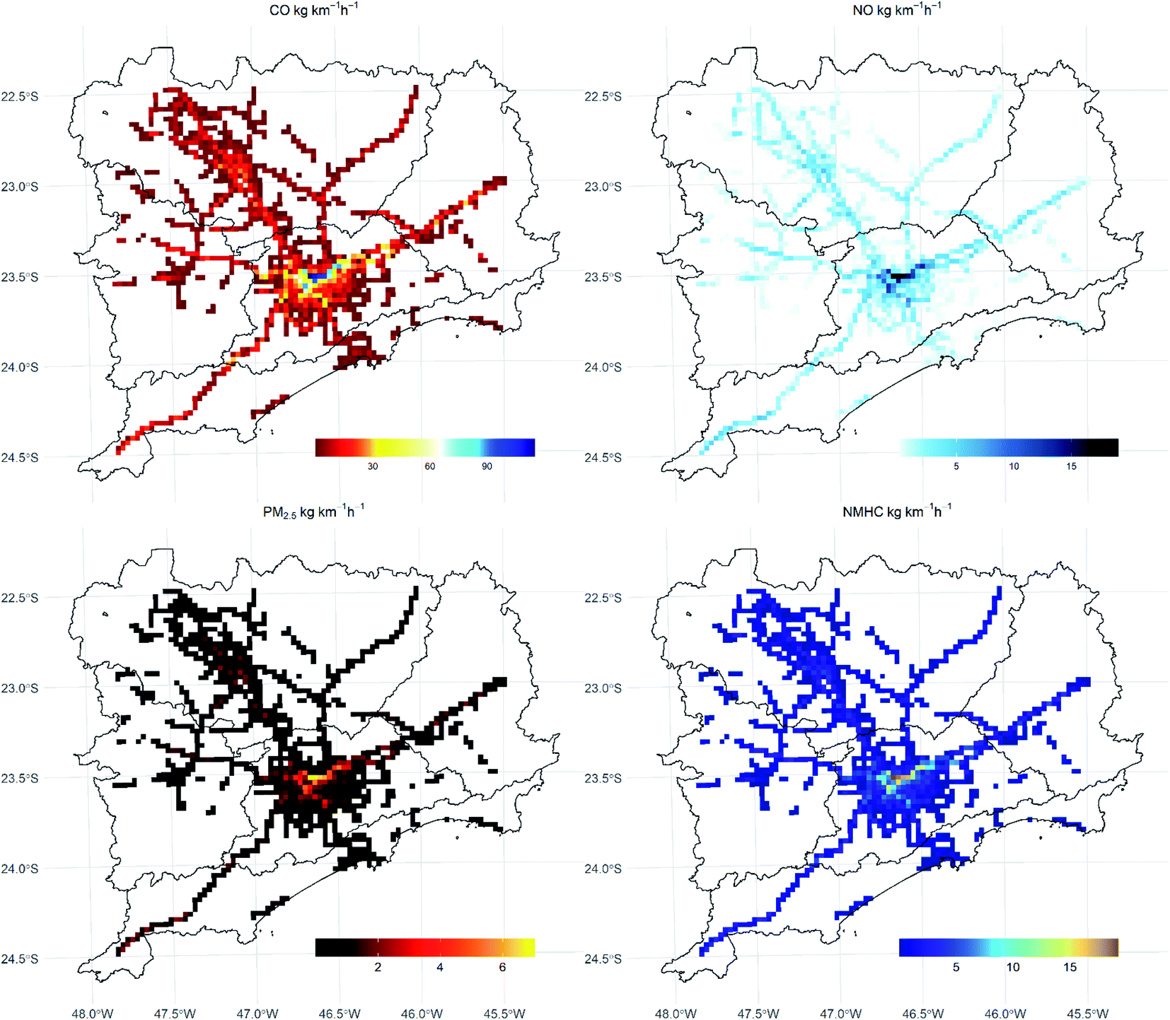 | ||
| Fig. 3 Emission flux of CO, NO, PM2.5 and NMHC (kg km−2 h−1) 08:00–09:00. These grids were generated using the numerical grids in WRF with a grid-spacing of 3 km. | ||
3.3. Air quality and meteorological modeling
The simulation variables precipitation (mm), 2 m relative humidity (%), wind speed at 10 m (m s−1), 2 meter temperature (°C), CO (ppm), O3 (μg m−3), PM10 (μg m−3), PM2.5 (μg m−3), NO (μg m−3), and NO2 (μg m−3) are shown in Fig. 4. The model evaluation is separated by dry and wet periods and includes the metropolitan areas of Campinas (CAMP), São Paulo (MASP), Santos (SAN), São José Dos Campos (SJDC), and Sorocaba (SOR). The surface observations are shown in red for the precipitation data (from INMET) and for the other variables (from CETESB) and in green and blue for the WRF-Chem simulations with and without aerosol feedbacks, respectively. The results in each metropolitan area include the average of all stations including the standard deviation as semi-transparent. The results show that the simulations are in agreement with observations in most cases as shown in Fig. 3. Furthermore, the correlations between observations and simulations were statistically highly significant (p-value < 0.001). For instance, the mean correlation for 2 m temperature, 2 meter relative humidity, wind speed, and precipitation was 0.92, 0.85, 0.75, and 0.49 for the dry period and 0.80, 0.79, 0.61, and 0.42 for the wet period, respectively. The indices of correlation, mean bias, and root mean square error are available in ESI Fig. S2 to S9† for each region and station. The overall correlation for the pollutants CO, NO, NO2, O3, PM10, and PM2.5 was 0.63, 0.56, 0.63, 0.53, 0.37, and 0.46 for the dry period, while for the wet period it was 0.35, 0.55, 0.57, 0.58, 0.36, and 0.37, respectively. Therefore, in general there is agreement between observations and simulations. | ||
| Fig. 4 Observations and WRF simulations with and without radiative feedbacks for precipitation (mm h−1), relative humidity (%), wind speed at 10 m (m s−1), and 2 m temperature (°C). Source data: INMET for precipitation and CETESB for the other variables. A two day spin-up time was considered for each period. | ||
As mentioned before, there is high spatial variability in the results. Fig. 5 reinforces the analysis of the impact of aerosol on meteorological and air pollutant variables, through the environmental variables with the difference of the values after activating the aerosol effect for each study period, including downward shortwave flux at the ground surface (SW), precipitation (PP), relative humidity (RH), planetary boundary layer (PBL), air temperature (T2), and vertical velocity (W). We included polygons denoting areas where the difference was significant applying Wilcoxon's test.67,68
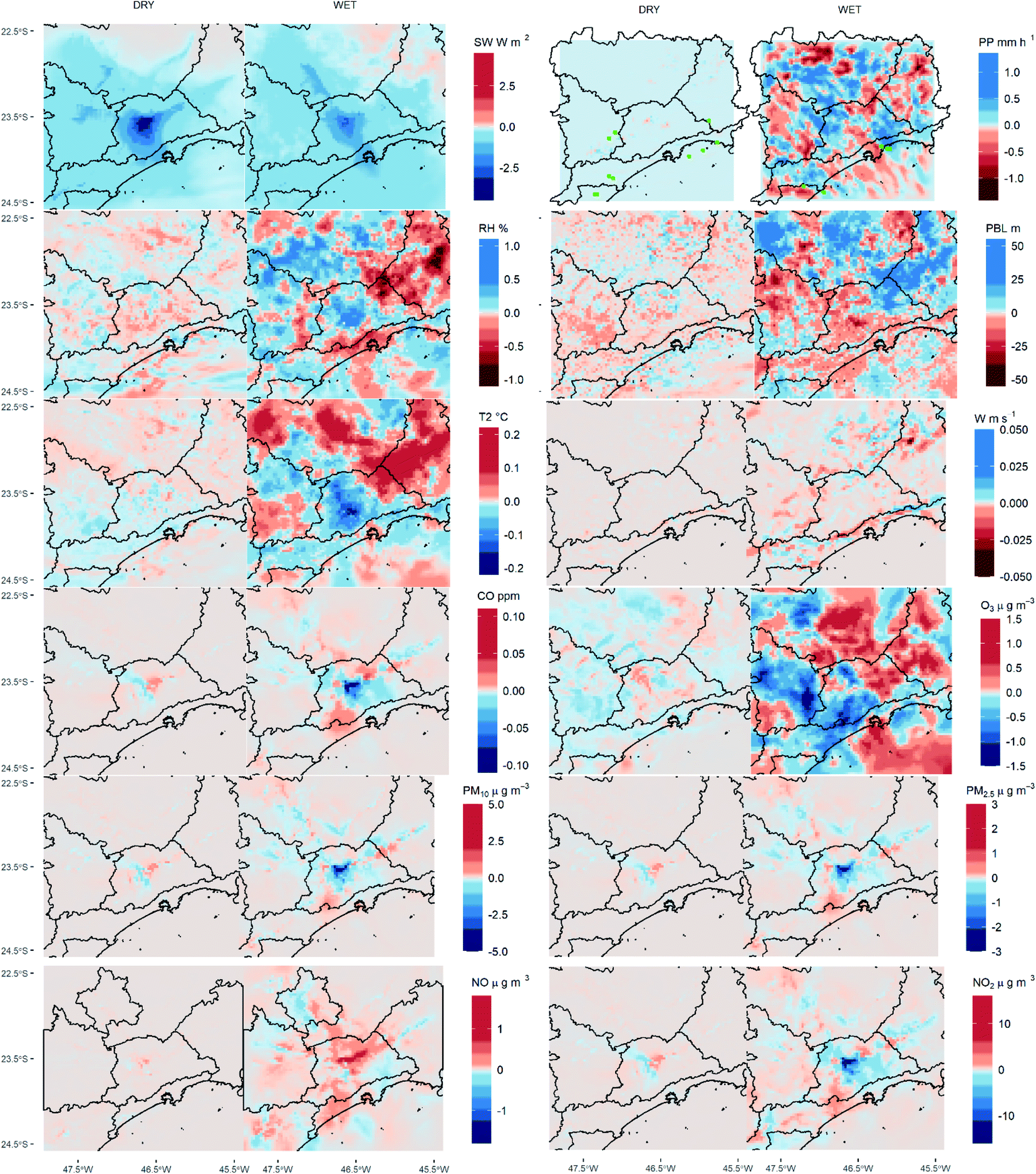 | ||
| Fig. 5 Differences of the environmental variables after activating the aerosol effect during the dry and wet periods. The SW, PP, RH, PBL, T2, and W are the downward shortwave fluxes at the ground surface, precipitation, relative humidity, planetary boundary layer, air temperature, and vertical velocity, respectively. A two-day spin-up time was considered for each period. | ||
The downward solar radiation is more impacted by aerosols during the dry period than the wet ones with a mean difference of −0.45 W m−2 up to −4.4 W m−2. This reduction represents a mean of 0.12% up to 1.27% less solar radiation at the surface. As the main source of particulate matter is resuspension, followed by the exhaust of diesel vehicles, the direct effect of aerosols on radiation follows the spatial distribution, with a stronger effect at the center of each urban area. When we consider the hourly variation at each pixel, the average is −0.44 W m−2 up to −24 W m−2 at the MASP center, representing 0.2% up to 12.5% less solar radiation during the dry period. The results for the wet period show a smaller effect of aerosols, on average −0.42 W m−2, representing a reduction of only 0.12%. An increase of solar radiation was simulated over the northeast part of the domain in response to the distancing from the emission sources inserted as input into the model. During the dry period, all the variables presented small differences but in the case of precipitation, some areas had significant differences. The precipitation presented an increase over MASP, CAMP, and SOR, and also presented a marked decrease over the north of CAMP. Furthermore, there are three small rectangles where the change in precipitation was significant. The average difference in precipitation shows an average increment of 10.73%, shown with green color.
The relative humidity shows a similar pattern of precipitation in most parts of the domain, however, during the dry period it's clear that MASP is less humid, while on the wet days, there is more humidity in MASP and CAMP, and less humidity in SJDC and SAN. However, the magnitude of these changes was only around 1% for the wet period and less than 1% for the dry period. The height of the planetary boundary layer was lower in all areas during the dry period in general, while during the wet period, the height increased up to 50 m in SJDC and decreased also up to 50 m on a location center-south of MASP. On average, the PBL decreased 0.3 m with a minimum of −16.15 m and a maximum of 13.83 m during the dry period. However, during the wet period, the average was 2.44 m with a minimum of −41.88 m in the west of MASP and an increase of 54 m between the east of MASP and SJDC, representing an increment of 4.9%. The 2 m temperature shows a pattern of lower temperature on the west side of the domain and higher temperatures on the east side with the same pattern but stronger during the wet period, with a marked decrease in MASP and an increase in SJDC. During the dry period the change in temperature was negligible, and during the wet period an increase of 0.01 °C, with a minimum of −0.19 °C and a maximum of 0.21 °C was observed. The vertical component of wind, W, was more affected during the wet period, with an average percentage change of −10.66%.
Some changes in meteorological variables resulted in important changes in air pollutant concentrations, more evident during the wet days. The changes over the dry days are primarily due to changes in radiation and the changes during the wet days are due to changes in PBL triggered by the indirect effect of aerosols on clouds. During the dry days, CO only changed in the MASP center, with a slight increase by 3% in the center-to-east and a decrease by 3% in the east, approximately. During the wet period, CO decreased strongly over the urban centers (0.1 ppm) and increased in the south and north of MASP (also 0.1 ppm) by around 10% and 20%, respectively. The O3 concentration decreased in the northwest and west parts of the domain during the dry period, while for wet ones there was a pattern of less O3 in the west part of the domain and higher concentrations of O3 in the northeast with changes up to 1.5 μg m−3. A stronger reduction of O3 of about 1.5% during the dry period occurs in the north of the domain while over the center of MASP, reductions of less than 1% and increments surrounding the center of about 1% were observed. During the wet period, the pattern of less O3 persists with an average reduction of 0.017 μg m−3 and 1.5 μg m−3 in Sorocaba and in the southwest of MASP. However, there were some increments in the northern part of the domain where the O3 concentrations were very small, which led to more than 10% of increment in that area. PM10 and PM2.5 presented a similar pattern with lower concentrations over downtown in each region, with more strong magnitudes up to −5 μg m−3 for PM10 and 3 μg m−3 for PM2.5. However, there are local increments of particulate matter. During the dry period, PM10 presented a modest increase over the center-eastern part of MASP of about 1 μg m−3 and less PM10 in other areas. As a result, the average percentage change was a reduction of 0.04% with a strong reduction of 20% on the coastline in the SAN region. During the wet period, the average reduction was 0.03 μg m−3 and about 5 μg m−3 over MASP downtown. In addition, the average percentage change was 1.14% over the Atlantic Ocean and also over other two locations, one in the western region between MASP and SAN and another in the northern part of the domain. The PM2.5 values followed the same pattern as PM10 for both periods. The changes of NO and NO2 were clearly simulated during the wet days, with higher NO concentrations over MASP, followed by urban motorways Marginal-Tiete and Ayrton-Senna with increases up to 1 μg m−3 while NO2 decreased substantially (by more than 10 μg m−3) at MASP downtown. NO2 during the dry period increased in general over the domain, and stronger reductions with more than 10% were found over the coastline in SAN. During the wet period, there was also an average reduction of 0.1 μg m−3. Regarding the percentage change, there were reductions of about 15% over downtown regions of MASP and SJDC and also over the eastern part of SAN, while stronger increments of about 25% were found over the Atlantic Ocean and the northern part of MASP. Finally, NO presented a strong increment during both periods. During the dry period, there was a modest increment in the MASP center, of more than 0.1 μg m−3, which represents on average 2.21% more NO.
The average wind speed and direction are shown in Fig. 6 for dry (top) and wet (bottom) periods, including also the difference with and without aerosol feedbacks. During the dry days, dominant wind flowed from the east quadrant over the analyzed regions while for the wet ones, the predominant direction is from the southeast. The wind speed over the ocean was above 8 m s−1 during the dry period and about 5 m s−1 during the wet period, while over the continent, winds are slower, with values of about 2–5 m s−1. It is possible to see that during the wet period the wind follows the coastline, in the division between MASP and SAN which represents a sea-breeze region. The effect of aerosols is weaker during the dry period, while during the wet ones, stronger differences are found in the north part of the domain, over SOR and also, over the southwest part. Furthermore, over the wet period, the band of higher speed between MASP and SOR is located slightly in the northeast part of the domain.
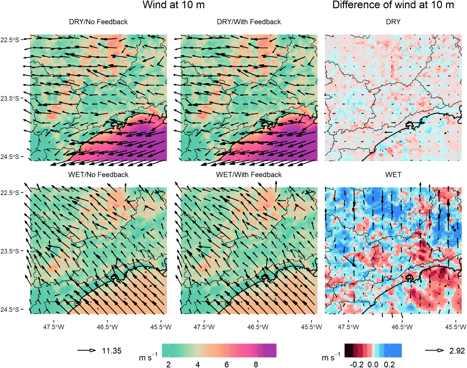 | ||
| Fig. 6 Wind speed (m s−1) and wind direction (degrees) averages over dry (top) and wet (bottom) periods associated with the simulations without (left) and with (middle) aerosol effects as well the differences among them (right). | ||
4. Discussion
Two WRF-Chem simulations were performed to study the aerosol feedback effects on meteorology and air quality over southeastern Brazil. To that end, study periods with (wet) and without (dry) rain between October and November of 2014 were selected for the model simulations. Even though the particulate matter is underrepresented due to missing bottom-up emission estimates from other sources (construction sites, fires, etc.), the effect of aerosols on radiation was noticed, being stronger during the dry period, as expected. In this sense, a mean reduction of 0.44 W m−2 occurred during the dry period. For other more polluted regions and including all aerosol sources, a stronger reduction, as in Forkel et al. (2015), of −1 W m−2 during boreal summer over Europe or −10 W m−2 in India can be found.69 In addition, solar radiation reduction over urban centers was up to 1.27%, while Zhang et al.70 found reductions of 4.1–5.6% in Texas, USA, a region that exceeds the national O3 air quality standards, similar to the cities in our study area. The simulation including the aerosol feedbacks showed that the precipitation presented an average enhancement of 10.73%, which is in line with other studies such as the study conducted by Guo et al. (2014) where an increment of 17% was found over China. In the case of PBL, Forkel et al. (2015) found a reduction of 5–8 m over Europe while in our study we found a decrease of −0.3 m with a minimum of −16.15 m and a maximum of 13.83 m. 2 m temperature presented variations between −0.19 and 0.21 °C during the wet period while Zhang et al. (2010) found variations between −1.3 and 1.4 °C over Texas, USA. Wind speed presented stronger variations due to aerosol effects during the wet period, with magnitudes up to 3 m s−1, with increments in most urban centers with the exception of MASP. In Quito, Ecuador, Parra71 found that including aerosol effects decreased solar radiation, increased surface temperature, enhanced PBL and decreased O3 concentrations. In a study made in the Iberian Peninsula centered in Portugal, Silveira et al.72 found that aerosols decrease solar radiation between 20 W m−2 and 40 W m−2, which resulted in about −0.5 °C. Finally, a study which investigated the effects of the Eyjafjallajökull volcano in south Iceland found that aerosols decrease the temperature between 1 and 2 because of less solar radiation in Europe.73 In general, we can see that our results align with the literature. However, further research is needed to evaluate the effects of aerosols including a comprehensive emission inventory for Brazil. The lack of comprehensive local emission inventories is seen in many countries in Latin America and Africa. Therefore, more efforts are needed to fill these gaps to improve the understanding of atmospheric chemistry.Air pollutant concentrations simulated with WRF-Chem align with observations in general. However, biases shown in the supplementary material indicate that the emissions need to be adjusted to further improve agreement observations. Although the main source of pollution in this region is vehicles, the inclusion of other sources is needed to better characterize air pollution. For instance, it has been shown that local restaurants may be responsible for a great part of PM emissions.74 Currently, there is ongoing work to develop a comprehensive and multi-year inventory for Brazil, being done by the authors.
Air pollutant concentrations are directly and indirectly affected by the effects of aerosols. In our study, stronger variations were found during the wet period. NO2 was underpredicted in most regions, with the exception of MASP, while NO is under-represented in all regions. However, our results are consistent with Forkel et al. (2015), who found reductions of CO, NO2, O3, PM10, and PM2.5 in the west part of urban centers. In addition, Vara-Vela et al. (2016) found a 2% reduction of O3 associated with the inclusion of the aerosol radiation feedback effect while we found a 1.5% reduction. NO2 presented a reduction, similar to the results found by Parra.71 NO was the only pollutant with a considerable increment over urban centers during both periods.
During the wet days, there was a dipole-type spatial pattern with less precipitation and humidity and more O3 over SJDC while more precipitation and humidity and less CO, NO2, PM2.5, and PM10 over MASP downtown were observed. This spatial pattern was modulated by the precipitation organization during this period, but more studies are needed to confirm if this pattern persists. It is important to highlight that this study aims at investigating the impact of vehicular emissions on air quality and the feedback effect of aerosols, but obviously, the next step would be to include all possible missing sources with a bottom-up estimation to account for spatial variability. We found no significant differences with the inclusion of aerosol feedback effects with the exception of enhanced precipitation over some locations in our study area during the wet period. We did find significant differences in precipitation, wind speed and direction, and in concentrations of CO and O3.
5. Conclusions
It has been shown that urbanization and air pollutant concentrations play a key role in daily precipitation extremes over wet periods in MASP.75 The updated urban vehicular emission inventory allowed a numerical representation of air pollutants which aligned with observations. It was found that the aerosols decreased solar radiation, temperature and O3 concentrations, as documented in previous studies. However, the aerosol effect was stronger during the wet period associated with the enhanced PBL. Specifically, after selecting the rainiest days, we did find a significant effect of aerosols, which means that more research is needed to cover a longer time span. Severe weather and mesoscale convective systems are atmospheric mechanisms responsible for a large part of precipitation over Southeast Brazil.76–78 In addition, the interactions of mesoscale convective systems, precipitation and air pollution need to be better understood, especially in urban areas.Conflicts of interest
None.Acknowledgements
G. A. M. da Silva is thankful for the financial support by the National Council for Scientific and Technological Development (CNPq, Grant N°. 426221/2016-8). E. D. F. efforts were supported by the São Paulo Research Foundation (FAPESP) (Grants N°. 2015/03804-9 and 2016/18438-0) and CNPq (Grant N° 309514/2019-3); A. R. efforts were also supported by FAPESP (Grant N°. 2016/10557-0 and 2021/07992-5); S. I. E. efforts were also supported by FAPESP (Grant N°. 2021/07136-1). This research was funded in part by the Wellcome Trust, U. K., with subaward from Yale University to Northeastern University (subcontract number GR108374). The authors also thank “Coordenação de Aperfeiçoamento de Pessoal de Nível Superior – Brasil” (CAPES) Finance Code 001.References
- G. P. Brasseur and D. J. Jacob, Modeling of Atmospheric Chemistry, Cambridge University Press, 2017 Search PubMed.
- D. Alvim, L. Gatti, S. Correa, J. Chiquetto, G. Santos and C. de Souza Rossatti, et al., Determining VOCs Reactivity for Ozone Forming Potential in the Megacity of São Paulo, Aerosol Air Qual. Res., 2018, 18, 2460–2474 CrossRef CAS.
- G. Hoshyaripour, G. Brasseur, M. de F. Andrade, M. Gavidia-Calderón, I. Bouarar and R. Y. Ynoue, Prediction of ground-level ozone concentration in São Paulo, Brazil: deterministic versus statistic models, Atmos. Environ., 2016, 145, 365–375 CrossRef CAS.
- J. D. Fast, W. I. Gustafson, R. C. Easter, R. A. Zaveri, J. C. Barnard and E. G. Chapman, et al., Evolution of ozone, particulates, and aerosol direct radiative forcing in the vicinity of Houston using a fully coupled meteorology-chemistry-aerosol model, J. Geophys. Res., D: Atmos., 2006, 111(21), D21305 CrossRef.
- J. E. Penner, M. O. Andreae, H. Annegarn, L. Barrie, J. Feichter and D. Hegg, et al., Aerosols, their direct and indirect effects, in, Climate Change 2001: the Scientific Basis Contribution of Working Group I to the Third Assessment Report of the Intergovernmental Panel on Climate Change, Cambridge University Press, 2001. pp. 289–348 Search PubMed.
- D. Rosenfeld, S. Sherwood, R. Wood and L. Donner, Climate effects of aerosol-cloud interactions, Science, 2014, 343(6169), 379–380 CrossRef CAS PubMed.
- D. Rosenfeld, U. Lohmann, G. B. Raga, C. D. O'Dowd, M. Kulmala and S. Fuzzi, et al., Flood or drought: How do aerosols affect precipitation?, Science, 2008, 321(5894), 1309–1313 CrossRef CAS PubMed.
- R. Forkel, A. Balzarini, R. Baró, R. Bianconi, G. Curci and P. Jiménez-Guerrero, et al., Analysis of the WRF-Chem contributions to AQMEII phase2 with respect to aerosol radiative feedbacks on meteorology and pollutant distributions, Atmos. Environ., 2015, 115, 630–645 CrossRef CAS.
- X. Guo, D. Fu, X. Guo and C. Zhang, A case study of aerosol impacts on summer convective clouds and precipitation over northern China, Atmos. Res., 2014, 142, 142–157 CrossRef CAS.
- K. M. Longo, A. M. Thompson, V. W. J. H. Kirchhoff, L. A. Remer, S. R. De Freitas and M. A. F. S. Dias, et al., Correlation between smoke and tropospheric ozone concentration in Cuiabá during Smoke, Clouds, and Radiation-Brazil (SCAR-B), J. Geophys. Res., D: Atmos., 1999, 104(10), 12113–12129 CrossRef CAS.
- P. J. Landrigan, R. Fuller, N. J. R. Acosta, O. Adeyi, R. Arnold and N. Basu, et al., The Lancet Commission on pollution and health, Lancet, 2018, 391(10119), 462–512 CrossRef.
- D.-H. Tsai, M. Riediker, A. Berchet, F. Paccaud, G. Waeber and P. Vollenweider, et al., Effects of short-and long-term exposures to particulate matter on inflammatory marker levels in the general population, Environ. Sci. Pollut. Res., 2019, 26(19), 19697–19704 CrossRef PubMed.
- WHO, Situation Report 1. Novel Coronavirus (2019-nCoV), World Health Organization, 2020, available from: https://www.who.int/docs/default-source/coronaviruse/situation-reports/20200121-sitrep-1-2019-ncov.pdf Search PubMed.
- P. M. ED. undiagnosed, Pneumonia – China, HUBEI: Request for Information, ProMED Post, 2019, cited 2021 Jul 29, available from: https://promedmail.org/promed-post/?id=6864153 Search PubMed.
- M. Meselson, N. van Doremalen, T. Bushmaker, D. H. Morris, M. G. Holbrook and A. Gamble, et al., Aerosol and Surface Stability of SARS-CoV-2 as Compared with SARS-CoV-1, N. Engl. J. Med., 2020, 382, 1564–1567 CrossRef PubMed.
- M. Meselson, Droplets and Aerosols in the Transmission of SARS-CoV-2, N. Engl. J. Med., 2020, 382, 2063 CrossRef PubMed.
- L. Morawska and J. Cao, Airborne transmission of SARS-CoV-2: The world should face the reality, Environ. Int., 2020, 139, 105730 CrossRef CAS PubMed , available from: http://www.sciencedirect.com/science/article/pii/S016041202031254X.
- L. Morawska and D. K. Milton, It Is Time to Address Airborne Transmission of Coronavirus Disease 2019 (COVID-19), Clin. Infect. Dis., 2020 DOI:10.1093/cid/ciaa939.
- L. Morawska, J. W. Tang, W. Bahnfleth, P. M. Bluyssen, A. Boerstra and G. Buonanno, et al., How can airborne transmission of COVID-19 indoors be minimised?, Environ. Int., 2020, 142, 105832 CrossRef CAS PubMed , available from: http://www.sciencedirect.com/science/article/pii/S0160412020317876.
- X. Wu, R. C. Nethery, M. B. Sabath, D. Braun and F. Dominici, Air pollution and COVID-19 mortality in the United States: Strengths and limitations of an ecological regression analysis, Sci. Adv., 2020, 6(45), eabd4049 CrossRef CAS PubMed.
- S. Ibarra-Espinosa, E. Dias de Freitas, K. Ropkins, F. Dominici and A. Rehbein, Negative-Binomial and quasi-poisson regressions between COVID-19, mobility and environment in São Paulo, Brazil, Environ. Res., 2021, 112369 Search PubMed , available from: https://www.sciencedirect.com/science/article/pii/S0013935121016704.
- I. B. GE. Instituto, Brasileiro de Geografia e Estatística – Estimativas da População, accessed 29 July 2021, 2020, available from: https://ftp.ibge.gov.br/Estimativas_de_Populacao/Estimativas_2020/estimativa_dou_2020.pdf:%20Online Search PubMed.
- M. de F. Andrade, R. Y. Ynoue, E. D. Freitas, E. Todesco, A. Vara Vela and S. Ibarra, et al., Air quality forecasting system for Southeastern Brazil, Front. Environ. Sci. Eng., 2015, 3, 1–12 Search PubMed.
- J. B. Chiquetto, M. E. S. Silva, W. Cabral-Miranda, F. N. D. Ribeiro, S. A. Ibarra-Espinosa and R. Y. Ynoue, Air quality standards and extreme ozone events in the São Paulo megacity, Sustain, 2019, 11(13), 3725 CrossRef CAS.
- S. Ibarra-Espinosa, R. Y. Ynoue, K. Ropkins, X. Zhang and E. D. de Freitas, High spatial and temporal resolution vehicular emissions in south-east Brazil with traffic data from real-time GPS and travel demand models, Atmos. Environ., 2020, 222, 117136 CrossRef CAS.
- L. M. V. Carvalho and I. F. A. Cavalcanti, The South American Monsoon System (SAMS), in The Monsoons and Climate Change, Springer, 2016, pp. 121–48 Search PubMed.
- J. Zhou and K. M. Lau, Does a monsoon climate exist over South America?, J Clim, 1998, 11(5), 1020–1040 CrossRef.
- L. M. V. Carvalho, A. E. Silva, C. Jones, B. Liebmann, P. L. S. Dias and H. R. Rocha, Moisture transport and intraseasonal variability in the South America monsoon system, Clim. Dyn., 2011, 36(9), 1865–1880 CrossRef.
- G. A. M. da Silva and T. Ambrizzi, Summertime moisture transport over Southeastern South America and extratropical cyclones behavior during inter-El Niño events, Theor. Appl. Climatol., 2010, 101(3–4), 303–310 CrossRef.
- G. A. M. da Silva, T. Ambrizzi and J. A. Marengo, Observational evidences on the modulation of the South American Low Level Jet east of the Andes according the ENSO variability, Ann. Geophys., 2009, 645–657 CrossRef.
- G. A. M. da Silva, A. Drumond and T. Ambrizzi, The impact of El Niño on South American summer climate during different phases of the Pacific Decadal Oscillation, Theor. Appl. Climatol., 2011, 106(3–4), 307–319 CrossRef.
- S. R. Garcia and M. T. Kayano, Climatological aspects of Hadley, Walker and monsoon circulations in two phases of the Pacific Decadal Oscillation, Theor. Appl. Climatol., 2008, 91(1–4), 117–127 CrossRef.
- E. D. Freitas, C. M. Rozoff, W. R. Cotton and P. L. S. Dias, Interactions of an urban heat island and sea-breeze circulations during winter over the metropolitan area of São Paulo, Brazil, Boundary-Layer Meteorol., 2007, 122(1), 43–65 CrossRef.
- G. M. P. Perez and M. A. F. Silva Dias, Long-term study of the occurrence and time of passage of sea breeze in São Paulo, 1960--2009, Int. J. Bioclimatol. Biometeorol., 2017, 37, 1210–1220 Search PubMed.
- A. Vara-Vela, M. de Fátima Andrade, Y. Zhang, P. Kumar, R. Y. Ynoue and C. E. Souto-Oliveira, et al., Modeling of Atmospheric Aerosol Properties in the São Paulo Metropolitan Area: Impact of Biomass Burning, J. Geophys. Res.: Atmos., 2018, 123(17), 9935–9956 CAS.
- A. Vara-Vela, M. F. Andrade, P. Kumar, R. Y. Ynoue and A. G. Muñoz, Impact of vehicular emissions on the formation of fine particles in the São Paulo Metropolitan Area: a numerical study with the WRF-Chem model, Atmos. Chem. Phys., 2016, 16, 777–797 CrossRef CAS.
- M. Gavidia-Calderón, A. Vara-Vela, N. M. Crespo and M. F. Andrade, Impact of time-dependent chemical boundary conditions on tropospheric ozone simulation with WRF-Chem: An experiment over the Metropolitan Area of São Paulo, Atmos. Environ., 2018, 195, 112–124 CrossRef.
- E. D. S. F. Duarte, P. Franke, A. C. Lange, E. Friese, F. J. da Silva Lopes and J. J. da Silva, et al., Evaluation of atmospheric aerosols in the metropolitan area of São Paulo simulated by the regional EURAD-IM model on high-resolution, Atmos. Pollut. Res., 2021, 12(2), 451–469 CrossRef.
- M. Gavidia-Calderón, S. Ibarra-Espinosa, Y. Kim, Y. Zhang and M. F. Andrade, Simulation of O3 and NOx in Sao Paulo street urban canyons with VEIN (v0.2.2) and MUNICH (v1.0), Geosci. Model Dev. Discuss., 2020, 14(1), 3251–3268 Search PubMed.
- S. Ibarra-Espinosa, R. Ynoue, S. O'Sullivan, E. Pebesma, M. D. F. Andrade and M. Osses, VEIN v0.2.2: an R package for bottom-up vehicular emissions inventories, Geosci. Model Dev., 2018, 11(6), 2209–2229 CrossRef CAS.
- G. A. Grell, S. E. Peckham, R. Schmitz, S. A. McKeen, G. Frost and W. C. Skamarock, et al., Fully coupled “online” chemistry within the WRF model, Atmos. Environ., 2005, 39(37), 6957–6975 CrossRef CAS.
- G. J. Huffman, D. T. Bolvin, E. J. Nelkin and others, Integrated Multi-satellitE Retrievals for GPM (IMERG) Technical Documentation, NASA/GSFC Code 612, 2020, available from: https://gpm.nasa.gov/sites/default/files/2020-05/IMERG_ATBD_V06.3.pdf Search PubMed.
- S. Ibarra-Espinosa, R. Ynoue, M. Giannotti, K. Ropkins and E. D. de Freitas, Generating traffic flow and speed regional model data using internet GPS vehicle records, MethodsX, 2019, 6, 2065–2075 CrossRef PubMed.
- C. E. T. E. SB. Emissões, Veiculares no Estado de São Paulo 2018, 2019 Search PubMed.
- T. Nogueira, L. Y. Kamigauti, G. M. Pereira, M. E. Gavidia-Calderón, S. Ibarra-Espinosa and G. L. de Oliveira, et al., Evolution of Vehicle Emission Factors in a Megacity Affected by Extensive Biofuel Use: Results of Tunnel Measurements in São Paulo, Brazil, Environ. Sci. Technol., 2021, 55(10), 6677–6687 CrossRef CAS PubMed.
- M. E. Gavidia-Calderón, S. Ibarra-Espinosa, Y. Kim, Y. Zhang and M. D. F. Andrade, Simulation of O3 and NOx in São Paulo street urban canyons with VEIN (v0.2.2) and MUNICH (v1.0), Geosci. Model Dev., 2021, 14(6), 3251–3268 CrossRef , available from: https://gmd.copernicus.org/articles/14/3251/2021/.
- US-EPA, AP-42: Compilation of Air Emissions Factors - Miscellaneous Sources – 13.2.1 Paved Roads, US-EPA, 2011, vol. 13, (2.1) Search PubMed.
- W. R. Stockwell, P. Middleton, J. S. Chang and X. Tang, The second generation regional acid deposition model chemical mechanism for regional air quality modeling, J. Geophys. Res., D: Atmos., 1990, 95(10), 16343–16367 CrossRef CAS.
- W. P. L. Carter, Development of a database for chemical mechanism assignments for volatile organic emissions, J. Air Waste Manage. Assoc., 2015, 65(10), 1171–1184 CrossRef CAS PubMed.
- D. Lancz, B. Szintai and R. Honnert, Modification of a Parametrization of Shallow Convection in the Grey Zone Using a Mesoscale Model, Boundary-Layer Meteorol, 2018, 169(3), 483–503 CrossRef.
- Y.-L. Lin, R. D. Farley and H. D. Orville, Bulk parameterization of the snow field in a cloud model, J. Clim. Appl. Meteorol., 1983, 22(6), 1065–1092 CrossRef.
- G. A. Grell and D. Dévényi, A generalized approach to parameterizing convection combining ensemble and data assimilation techniques, Geophys. Res. Lett., 2002, 29(14) DOI:10.1029/2002GL015311.
- E. J. Mlawer, S. J. Taubman, P. D. Brown, M. J. Iacono and S. A. Clough, Radiative transfer for inhomogeneous atmospheres: RRTM, a validated correlated-k model for the longwave, J. Geophys. Res., D: Atmos., 1997, 102(14), 16663–16682 CrossRef CAS.
- M.-D. Chou and M. J. Suarez, A solar radiation parameterization (CLIRAD-SW) for atmospheric studies, NASA Tech. Memo., 1999, 48 Search PubMed.
- M. Tewari, F. Chen, W. Wang, J. Dudhia, M. A. LeMone and K. Mitchell, et al., Implementation and verification of the unified NOAH land surface model in the WRF model, in 20th Conference on Weather Analysis and Forecasting 16th Conference on Numerical Weather Prediction, 2004, pp. 1–6 Search PubMed.
- S.-Y. Hong, Y. Noh and J. Dudhia, A new vertical diffusion package with an explicit treatment of entrainment processes, Mon. Weather Rev., 2006, 134(9), 2318–2341 CrossRef.
- D. Zhang and R. A. Anthes, A high-resolution model of the planetary boundary layer—Sensitivity tests and comparisons with SESAME-79 data, J. Appl. Meteorol., 1982, 21(11), 1594–1609 CrossRef.
- S. Saha, S. Moorthi, H.-L. Pan, X. Wu, J. Wang and S. Nadiga, et al.NCEP Climate Forecast System Reanalysis (CFSR) 6-hourly Products, January 1979 to December 2020 Research Data Archive at the National Center for Atmospheric Research, Computational and Information Systems Laboratory, Boulder, CO, 2010, DOI:10.5065/D69K487J.
- F. Chen, H. Kusaka, R. Bornstein, J. Ching, C. S. B. Grimmond and S. Grossman-Clarke, et al., The integrated WRF/urban modelling system: development, evaluation, and applications to urban environmental problems, Int. J. Bioclimatol. Biometeorol., 2011, 31(2), 273–288 Search PubMed.
- P. A. Jiménez and J. Dudhia, Improving the representation of resolved and unresolved topographic effects on surface wind in the WRF model, J. Appl. Meteorol. Climatol., 2012, 51(2), 300–316 Search PubMed.
- I. J. Ackermann, H. Hass, M. Memmesheimer, A. Ebel, F. S. Binkowski and U. Shankar, Modal aerosol dynamics model for Europe: development and first applications, Atmos. Environ., 1998, 32(17), 2981–2999 CrossRef , available from: https://www.sciencedirect.com/science/article/pii/S1352231098000065.
- B. Schell, I. J. Ackermann, H. Hass, F. S. Binkowski and A. Ebel, Modeling the formation of secondary organic aerosol within a comprehensive air quality model system, J. Geophys. Res., D: Atmos., 2001, 106(22), 28275–28293 CrossRef CAS.
- CPTEC/INPE, Synoptic Charts for Southeamerica, 2021, available from: http://img0.cptec.inpe.br/%7Ergptimg/Produtos-Pagina/Carta-Sinotica/Analise/ Search PubMed.
- CPTEC/INPE, Satellite Division and Environment Systems (DSA), 2021[cited 2020 Jul 31], available from: http://satelite.cptec.inpe.br/acervo/goes.formulario.logic?i=en Search PubMed.
- C. E. T. E. SB. Emissões, Veiculares no Estado de São Paulo 2014, 2015 Search PubMed.
- S. Ibarra-Espinosa, D. Schuch and de F. E. eixport, An R package to export emissions to atmospheric models, J. Open Source Softw., 2018, 3(24), 6071–6074 Search PubMed.
- D. F. Bauer, Constructing confidence sets using rank statistics, J. Am. Stat. Assoc., 1972, 67(339), 687–690 CrossRef.
- R Core Team, R: A Language and Environment for Statistical Computing, Vienna, Austria, 2021, available from: https://www.r-project.org/ Search PubMed.
- J. Prakash, P. Vats, A. K. Sharma, D. Ganguly, G. Habib and others, New Emission Inventory of Carbonaceous Aerosols from the On-Road Transport Sector in India and Its Implications for Direct Radiative Forcing over the Region, Aerosol Air Qual. Res., 2020, 20(4), 741–761 CrossRef CAS.
- Y. Zhang, Y. Pan, K. Wang, J. D. Fast and G. A. Grell, WRF/Chem-MADRID: Incorporation of an aerosol module into WRF/Chem and its initial application to the TexAQS2000 episode, J. Geophys. Res., D: Atmos., 2010, 115(18) Search PubMed ), available from: https://agupubs.onlinelibrary.wiley.com/doi/abs/10.1029/2009JD013443.
- R. Parra, Performance studies of planetary boundary layer schemes in WRF-Chem for the Andean region of Southern Ecuador, Atmos. Pollut. Res., 2018, 9(3), 411–428 CrossRef CAS , available from: https://www.sciencedirect.com/science/article/pii/S1309104217302830.
- C. Silveira, A. Martins, S. Gouveia, M. Scotto, A. I. Miranda and A. Monteiro, The Role of the Atmospheric Aerosol in Weather Forecasts for the Iberian Peninsula: Investigating the Direct Effects Using the WRF-Chem Model, Atmosphere, 2021, 12(2) CrossRef CAS ), available from: https://www.mdpi.com/2073-4433/12/2/288.
- M. Hirtl, M. Stuefer, D. Arnold, G. Grell, C. Maurer and S. Natali, et al., The effects of simulating volcanic aerosol radiative feedbacks with WRF-Chem during the Eyjafjallajökull eruption, Atmos. Environ., 2019, 198, 194–206 CrossRef CAS , available from: https://www.sciencedirect.com/science/article/pii/S1352231018307568.
- P. Kumar, M. de Fatima Andrade, R. Y. Ynoue, A. Fornaro, E. D. de Freitas and J. Martins, et al., New directions: From biofuels to wood stoves: The modern and ancient air quality challenges in the megacity of São Paulo, Atmos. Environ., 2016, 140, 364–369 CrossRef CAS , available from: https://www.sciencedirect.com/science/article/pii/S1352231016304071.
- M. A. F. Silva Dias, J. Dias, L. M. V. Carvalho, E. D. Freitas and P. L. Silva Dias, Changes in extreme daily rainfall for São Paulo, Brazil, Clim. Change, 2013, 116(3), 705–722, DOI:10.1007/s10584-012-0504-7.
- A. Rehbein, L. M. M. Dutra, T. Ambrizzi, R. P. da Rocha, M. S. Reboita and G. A. M. da Silva, et al., Severe weather events over southeastern Brazil during the 2016 dry season, Adv Meteorol., 2018, 1–15 Search PubMed.
- A. Rehbein, T. Ambrizzi and C. R. Mechoso, Mesoscale convective systems over the Amazon basin. Part I: climatological aspects, Int. J. Bioclimatol. Biometeorol., 2018, 38(1), 215–229 Search PubMed.
- A. Rehbein, T. Ambrizzi, C. R. Mechoso, S. A. I. Espinosa and T. A. Myers, Mesoscale convective systems over the Amazon basin: The GoAmazon2014/5 program, Int. J. Bioclimatol. Biometeorol., 2019, 39(15), 5599–5618 Search PubMed.
Footnotes |
| † Electronic supplementary information (ESI) available. See DOI: 10.1039/d1ea00080b |
| ‡ https://atmoschem.github.io/vein/reference/ef_cetesb.html |
| § https://atmoschem.github.io/vein/reference/emis_chem2.html |
| ¶ https://atmoschem.github.io/vein/reference/emis_grid.html |
| This journal is © The Royal Society of Chemistry 2022 |