DeepAC – conditional transformer-based chemical language model for the prediction of activity cliffs formed by bioactive compounds

Abstract

Activity cliffs (ACs) are formed by pairs of structurally similar or analogous active small molecules with large differences in potency. In medicinal chemistry, ACs are of high interest because they often reveal structure–activity relationship (SAR) determinants for compound optimization. In molecular machine learning, ACs provide test cases for predictive modeling of discontinuous (non-linear) SARs at the level of compound pairs. Recently, deep neural networks have been used to predict ACs from molecular images or graphs via representation learning. Herein, we report the development and evaluation of chemical language models for AC prediction. It is shown that chemical language models learn structural relationships and associated potency differences to reproduce ACs. A conditional transformer termed DeepAC is introduced that accurately predicts ACs on the basis of small amounts of training data compared to other machine learning methods. DeepAC bridges between predictive modeling and compound design and should thus be of interest for practical applications.

---

1 Introduction

In medicinal chemistry, compound optimization relies on the exploration of structure–activity relationships (SARs). Therefore, series of structural analogues are generated to probe substitution sites in specifically active compounds with different functional groups and improve potency and other lead optimization-relevant molecular properties. For lead optimization, the activity cliff (AC) concept plays an important role. ACs are defined as pairs or groups of structurally similar compounds or structural analogues that are active against a given target and have large differences in potency.^1–3 As such, ACs represent strongly discontinuous SARs because small chemical modifications lead to large biological effects. In medicinal chemistry, SAR discontinuity captured by ACs helps to identify substituents that are involved in critically important ligand–target interactions. In compound activity prediction, the presence of SAR discontinuity prevents the derivation of quantitative SAR (QSAR) models relying on continuous SAR progression and requires non-linear machine learning models.^1,2

For a non-ambiguous and systematic assessment of ACs, similarity and potency difference criteria must be clearly defined.^2,3 Originally, molecular fingerprints (that is, bit string representations of chemical structure) have been used as molecular representations to calculate the Tanimoto coefficient,⁴ a whole-molecule similarity metric, for identifying similar compounds forming ACs.² Alternatively, substructure-based similarity measures have been adapted for defining ACs, which have become increasingly popular in medicinal chemistry, because they are often chemically more intuitive than calculated whole-molecule similarity.³ For example, a widely used substructure-based similarity criterion for AC analysis is the formation of a matched molecular pair (MMP), which is defined as a pair of compounds that are only distinguished by a chemical modification at a single site.⁵ Thus, MMPs can be used to represent pairs of structural analogues, which explains their popularity in medicinal chemistry. Moreover, MMPs can also be efficiently identified algorithmically.⁵ Although statistically significant potency differences for ACs can be determined for individual compound activity classes,⁶ for the systematic assessment of ACs and computational modeling, a potency difference threshold of at least two orders of magnitude (100-fold) has mostly been applied.^2,3

While medicinal chemistry campaigns encounter ACs on a case-by-case basis, systematic compound database analysis has identified ACs across different compound activity classes, providing a wealth of SAR information.^2,7 Here, computational and medicinal chemistry meet. With rapidly increasing numbers of publicly available bioactive compounds, AC populations have also grown over time.³ However, the rate at which ACs are formed across different activity classes has essentially remained constant. Only ∼5% of pairs of structural analogues sharing the same activity form ACs across different activity classes.^3,7 Thus, as expected for compounds representing the pinnacle of SAR discontinuity, structural analogues rarely form ACs.

Systematic identification of ACs across activity classes has also provided the basis for computational predictions of ACs. For machine learning, AC predictions generally present a challenge, for three reasons. First, as discussed, the underlying SARs that need to be accounted for are highly discontinuous; second, data sets of ACs and non-ACs are unbalanced; third, predictions need to be made at the level of compound pairs, rather than individual compounds, which is usually the case in compound classification or molecular property prediction. Initial attempts to predict ACs were reported a decade ago.^8,9 ACs were first accurately predicted using support vector machine (SVM) modeling on the basis of special kernel functions enabling compound pair predictions.⁹ These findings have also catalyzed further AC predictions using SVR variants^10–12 and other methods,^13–18 as discussed below. Recently, various deep neural network architectures have been used to predict ACs from images^14,15 and molecular graphs using representation learning¹⁶ or derive regression models for potency prediction of AC compounds.^17,18

In this work, we further extend this methodological spectrum by introducing chemical language models for combined AC prediction and generative compound design. Compared to earlier studies predicting ACs using classification models, the approach presented herein was designed to extend AC predictions with the capacity to produce new AC compounds, thus integrating predictive and generative modeling in the context of AC analysis and AC-based compound design.

2 Methods

2.1 Compounds and activity data

Bioactive compounds with high-confidence activity data were assembled from ChEMBL (version 26).¹⁹ The following selection criteria were applied. Only compounds involved in direct interactions with human targets at the highest assay confidence level (assay confidence score 9) were selected and only numerically specified equilibrium constants (K_i values) were accepted as potency measurements. Equilibrium constants were recorded as (negative logarithmic) pK_i values. Multiple measurements for the same compound were averaged, provided all values fell within the same order of magnitude; if not, the compound was disregarded. Hence, in a given class, all compounds were active against a specific target. Compounds were represented using molecular-input line-entry system (SMILES) strings.²⁰

2.2 Matched molecular pairs

From activity classes, all possible MMPs were generated by systematically fragmenting individual exocyclic single bonds in compounds and sampling core structures and substituents in index tables.⁵ For substituents, size restrictions were applied to limit MMP formation to structural analogues typical for medicinal chemistry. Accordingly, a substituent was permitted to contain at most 13 non-hydrogen atoms and the core structure was required to be at least twice as large as a substituent. In addition, for MMP compounds, the maximum difference in non-hydrogen atoms between the substituents was set to eight, yielding transformation size-restricted MMPs.²¹ The systematic search identified 357 343 transformation size-restricted MMPs originating from a total of 600 activity classes.

2.3 Data set for model derivation

From the MMPs, a large general data set for model training was assembled by combining 338 748 MMPs from 596 activity classes. The majority of MMPs captured only minor differences in potency. Importantly, model pre-training, as specified below, did not require the inclusion of explicit target information because during this phase, the model must learn MMP-associated potency differences caused by given chemical transformations. Each MMP represented a true SAR, which was of critical relevance in this context, while target information was not required for pre-training. By contrast, subsequent fine-tuning then focused the model on target-specific activity classes for AC prediction and compound design.

MMPs comprising the general data set were represented as triples:

(Compound_A, Compound_B, Potency_B − Potency_A).

Compound_A represented the source compound that was concatenated with the potency difference (Potency_B − Potency_A) while Compound_B represented the target compound. Each MMP yielded two triples, in which each MMP compound was used once as the source and target compound, respectively. The source and target compounds were then used as the input and associated output for model training, respectively. Furthermore, for MMP-triples, data ambiguities could arise if an MMP was associated with multiple potency values for different targets or if a given source compound and potency difference was associated with multiple target compounds from different activity classes. Such MMPs were eliminated. Finally, for the general data set, a total of 338 748 qualifying MMP-triples were obtained.

For modeling, MMP-triples were randomly divided into training (80%), validation (10%), and test (10%) sets. Source and target compounds from MMP-triples displayed nearly indistinguishable potency value distributions.

For the initial evaluation of chemical language models, three different test (sub)set versions were designed:

(i) Test-general: complete test set of 33 875 MMP-triples excluded from model training.

(ii) Test-core: subset of 2576 test set MMP-triples with core structures not present in training compounds.

(iii) Test-sub: subset of 14 193 MMP-triples with substituents (R-groups) not contained in training compounds.

For the generation of the training subsets, compounds were decomposed into core structures and substituents via MMP fragmentation.⁵

2.4 Activity cliffs

For ACs, the MMP-Cliff definition was applied.²¹ Accordingly, a transformation size-restricted MMP from a given activity class represented an AC if the two MMP-forming compounds had a potency difference of at least two orders of magnitude (100-fold; i.e., ΔpK_i ≥ 2.0). MMP-Cliffs were distinguished from “MMP-nonCliffs”, that is, pairs of structural analogues not representing an AC. To avoid potency boundary effects in AC prediction, compounds forming an MMP-nonCliff were restricted to a maximal potency difference of one order of magnitude (10-fold; ΔpK_i ≤ 1). Hence, MMPs capturing potency differences between 10- and 100-fold were not considered for AC prediction.

MMP-Cliffs and MMP-nonCliffs were extracted from four large activity classes including inhibitors of thrombin (ChEMBL ID 204) and tyrosine kinase Abl (1862) as well as antagonists of the Mu opioid receptor (233) and corticotropin releasing factor receptor 1 (1800). For MMP-Cliffs and MMP-nonCliffs, triples were ordered such that Compound_A had lower potency than (or equal potency to) Compound_B. These activity classes were excluded from the general data set and their MMP-Cliffs and MMP-nonCliffs thus formed an external/independent test set for AC prediction (Table 1).

Table 1 Compound activity classes for activity cliff prediction

Target name	ChEMBL ID	Total MMPs	MMP- Cliffs	MMP-nonCliffs
Thrombin	204	4249	438	2976
Mu opioid receptor	233	5875	329	4319
Tyrosine kinase Abl	1862	5403	564	3093
Corticotropin releasing factor receptor 1	1800	3068	317	1889

---

2.5 Deep chemical language models

Chemical language models for AC prediction were designed to learn the following mapping from MMP-triples:

(Source compound, Potency difference) → (Target compound).

Then, given a new (Source compound, Potency difference) test instance, trained models were supposed to generate a set of target candidate compounds meeting the potency difference condition.

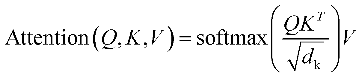
Sequence-to-sequence (Seq2Seq) models represent an encoder–decoder architecture to convert an input sequence (such as a character string) into an output sequence.²² These models can be adapted for a variety of applications, especially for neural machine translation.²² The encoder reads an input sequence and compresses it into a context vector as its last hidden state. The context vector serves as the input for the decoder network component that interprets the vector to predict an output sequence. Because long input sequences often present challenges for generating context vectors,²³ an attention mechanism²⁴ was introduced that utilizes hidden states from each time step of the encoder. As a further advance, a transformer neural network architecture was introduced that only relies on the attention mechanism.²⁵ The transformer architecture comprises multiple encoder–decoder modules (Fig. 1). An encoder module consists of a stack of encoding layers composed of two sub-layers including a multi-head self-attention sub-layer and a fully connected feed-forward network (FFN) sub-layer. Multi-head attention has multiple, single attention functions acting in parallel such that different positions in the input sequence can be processed simultaneously. The attention mechanism is based upon the following function:

Fig. 1 Architecture of a transformer encoder–decoder with attention mechanism.

The input for the attention layer is received in the form of three parameters including query (Q), keys (K), and values (V). In addition, a scaling factor d_k (equal to the size of weight matrices) prevents calculations of excessive dot products.²⁵ More details concerning the attention function are provided in the original literature of the transformer model.²⁵ The FFN sub-layer employs rectified linear unit (ReLU) activation.²⁶ The multi-head self-attention and FFN sub-layers are then linked via layer normalization²⁷ and a residual skip-connection.²⁸ Each decoder layer contains three sub-layers including an FFN sub-layer and two multi-head attention sub-layers. The first attention sub-layer was controlled by a mask function.

In this work, all source and target molecules were represented as canonical SMILES strings generated using RDKit²⁹ and further tokenized to construct a chemical vocabulary containing all the possible chemical tokens. The start and end of a sequence were represented by two special “start” and “end” tokens, respectively. For AC prediction, models must be guided towards the generation of compounds meeting potency difference constraints. Therefore, potency differences captured by MMPs were tokenized by binning.²³ The potency difference, ranging from −8.02 to 9.53, was partitioned into 1755 bins of width 0.01 that were also added to the chemical vocabulary. Each bin was encoded by a single token and each potency difference was assigned to the token of the corresponding bin (Fig. 1), e.g., a potency difference of 2.134 was encoded as ‘pK_i_change_(2.13, 2.14)’. Accordingly, the tokenization preserved the quantitative relationship between bins. The SMILES representation of a source compound combined with its potency difference token then represented the input sequence for the transformer encoder and was converted into a latent representation. Based on this representation, the transformer decoder iteratively generated output SMILES sequences until the end token was obtained. During training, the transformer model minimized the cross-entropy loss between the ground-truth target and output sequence.

2.6 Model derivation and selection

Seq2Seq and transformer models were implemented using Pytorch.³⁰ The Adam optimizer with learning rate 0.0001 and a batch size of 64 was applied. For transformer models, default hyperparameter settings were used,²⁵ except for the input and output encoding dimension, which was reduced from 512 to 256, and label smoothing, which was set to 0. On the basis of the general training set, models were derived over 200 epochs. A checkpoint was saved at each epoch and for the validation set, minimal loss was determined for selecting the final model. For the test set, generated candidate compounds were canonicalized using RDkit and compared to the target compounds.

2.7 Reference methods for activity prediction

For AC prediction, the chemical language models were compared to models of different machine learning methods including support vector machine (SVM),³¹ random forest (RF),³² and extreme gradient boosting (XGboost)³³ that were generated using scikit-learn.³⁴ As a molecular representation, the extended connectivity fingerprint with bond diameter of 4 (ECFP4) was used.³⁵ For the common core of an MMP and the two substituents defining the chemical transformation, fingerprint vectors were generated. For use of the MMP kernel,⁹ these vectors were concatenated to yield a single vector⁹ as input for deriving SVM, RF, and XGboost models. Hyperparameters of all models were optimized using the Hyperopt³⁶ package with five-fold cross-validation, as reported in Table 2.

Table 2 Hyperparameter settings for optimization of different models

Model	Hyperparameters	Value space for optimization
SVM	Kernel function	‘Linear’, ‘sigmoid’, ‘poly’, ‘rbf’, ‘tanimoto’
	C	1, 10, 100, 1000, 10 000
	Gamma	10^−6, 10^−5, 10^−4, 10^−3, 10^−2, 10^−1
RF	Max_depth	3, 4, 5, 6, 7, 8, 9, 10
	Max_features	32, 64, 128, 256, 512, 1024
	n_estimators	1, 2, 4, 8, 16, 32, 64, 100, 200
XGboost	Max_depth	3, 4, 5, 6, 7, 8, 9, 10
	n_estimators	1, 2, 4, 8, 16, 32, 64, 100, 200
	Learning_rate	0.0001, 0.001, 0.01, 0.1, 0.2, 0.3
	Subsample	0.5, 0.6, 0.7, 0.8, 0.9, 1
	Min_child_weight	0, 1, 2, 3, 4, 5

---

2.8 Evaluation metrics

A reproducibility criterion was introduced to measure the ability of a chemical language model to reproduce a target compound for a given source compound and potency difference. An MMP-triple met this criterion if it was reproduced when generating a pre-defined number of target candidate compounds. In our calculations, up to 50 distinct molecules were generated for each source compound to determine the reproducibility of a target compound, defined as:

MMP_test and MMP_repro denote the number of MMP-triples that were tested and reproduced by a model, respectively. Notably, this definition of reproducibility directly corresponds to the recall of labeled instances for classification models.

AC predictions were also evaluated by determining the true positive rate (TPR), true negative rate (TNR), and balanced accuracy (BA),³⁷ defined as:

TP, TN, FP, and FN denote true positives, true negatives, false positives, and false negatives respectively.

3 Results and discussion

3.1 Study concept

The basic idea underlying the use of chemical language models for AC prediction was learning the following mapping based on textual/string representations:

(Source compound, Potency difference) → (Target compound).

Then, given a new (Source compound, Potency difference) test instance, the pre-trained models should generate target compounds with appropriate potency. For deriving pairs of source and target compounds, the MMP formalism was applied. For AC prediction, pre-trained models were subjected to fine-tuning on MMP-Cliffs and MMP-nonCliffs from given activity classes, corresponding to the derivation of other supervised machine learning models.

3.2 Pre-trained chemical language models

Initially, the ability of Seq2Seq and transformer models to reproduce target compounds for test (sub)sets was evaluated by calculating the reproducibility measure. The results are summarized in Table 3. Therefore, for each test set triple, the source compound/potency difference concatenation was used as input and 50 target candidate compounds were sampled. Notably, the sampling procedure is an integral part of chemical language models in order to generate new candidate compounds, hence setting these models apart from standard class label prediction/classification approaches.

Table 3 Reproducibility of target compounds by chemical language models

	Test-general	Test-core	Test-sub
Seq2Seq	0.719	0.370	0.759
Transformer	0.818	0.528	0.850

---

For the entire test set, the Seq2Seq and transformer model achieved reproducibility of 0.719 and 0.818, respectively. Hence, the models were able to regenerate more than 70% and 80% of the target compounds from MMP-triples not used for training, respectively. However, reproducibility was consistently higher for the transformer and all training set versions than for the Seq2Seq model (Table 3). Hence, preference for AC prediction was given to the transformer. The test-general reproducibility of more than 80% was considered high. Attempting to further increase this reproducibility might compromise the ability of the model to generate novel compounds by strongly focusing on chemical space encountered during training. As expected, the test-core reproducibility was generally lowest because in this case, the core structures of MMPs were not available during training (limiting reproducibility much more than in the case of test-sub, i.e., evaluating novel substituents).

3.3 Fine-tuning for activity cliff prediction

The transformer was first applied to reproduce MMP-Cliffs and MMP-nonCliffs from the four activity classes excluded from pre-training. Therefore, for each MMP-triple, the source compound/potency difference concatenation was used as input for generating target compounds. As expected for activity classes not encountered during model derivation, reproducibility of MMP-Cliffs and MMP-nonCliffs was low, reaching maximally 5% for MMP-Cliffs and ∼19% for MMP-nonCliffs (Table 4).

Table 4 Reproducibility of MMP-Cliffs and MMP-nonCliffs by pre-trained DeepAC

Reproducibility	Activity classes
	ChEMBL204	1862	233	1800
MMP-Cliffs	0.050	0.007	0.049	0.006
MMP-nonCliffs	0.185	0.081	0.188	0.035

---

Therefore, a transfer learning approach was applied by fine-tuning the pre-trained transformer on these activity classes. For fine-tuning, 5%, 25%, and 50% of MMP-Cliffs and MMP-nonCliffs of each class were randomly selected. The resulting models were then tested on the remaining 50% of the MMP-Cliffs and MMP-nonCliffs.

Only 5% of the training data were required for fine-tuning to achieve reproducibility rates of 70% to greater than 80% for MMP-Cliffs from the different activity classes (Fig. 2A, solid lines). For MMP-nonCliffs, 25% of the training data were required to achieve reproducibility between 60% and 80% for the different classes (Fig. 2B, solid lines). For practical applications, these findings were encouraging because for any given target, there were many more MMP-nonCliffs available than MMP-Cliffs.

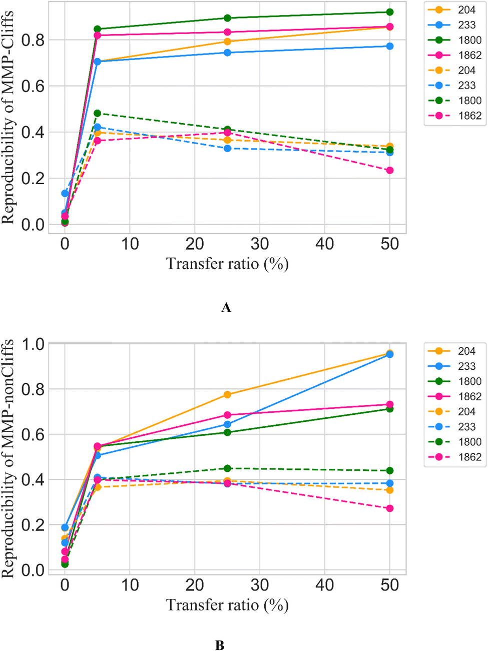Fig. 2 Reproducibility of MMP-Cliffs and MMP-nonCliffs after fine-tuning. For (A) MMP-Cliffs and (B) MMP-nonCliffs from different activity classes (identified by ChEMBL target IDs according to Table 1), reproducibility is reported as a function of transfer ratio accounting for the percentage of training data used for fine tuning. Solid lines represent results for true MMP-Cliffs and MMP-nonCliffs and dashed lines for control data obtained by inverting potency differences for MMP-Cliffs and MMP-nonCliffs.

Furthermore, to directly test whether high reproducibility achieved through fine-tuning only depended on learning structural relationships encoded by MMPs or if potency differences were also learned, a prerequisite for meaningful AC prediction, control calculations with inverted potency differences were carried out. Therefore, for all MMP-Cliffs, potency differences were set to ΔpK_i = 0.1 and for all MMP-nonCliffs, potency differences were set to ΔpK_i = 2.0. Using these hypothetical (SAR-nonsensical) data as test instances, reproducibility rates were determined again. In this case, reproducibility rates remained well below 50% for both MMP-Cliffs (Fig. 2A, dashed lines) and MMP-nonCliffs (Fig. 2B, dashes lines) and further decreased with increasing amounts of training data used for fine-tuning. These findings conclusively showed that the conditional transformer associated structural relationships with corresponding potency differences, thereby learning to reproduce and differentiate between MMP-Cliffs and MMP-nonCliffs.

In the following, the conditional transformer for AC prediction is referred to as DeepAC.

We also evaluated the capability of the model to reconstruct both MMP-Cliffs and MMP-nonCliffs originating from the same source compound. For each activity class, we compiled a set of source compounds from the original test data. Then, models were fine-tuned with varying amounts of data and applied to reproduce MMP-Cliff and MMP-nonCliff target compounds from the same source compound. As shown in Fig. 3, DeepAC reproduced more than 80% of the target compounds using 5%, 25%, or 50% of fine-tuning data, depending on the activity class.

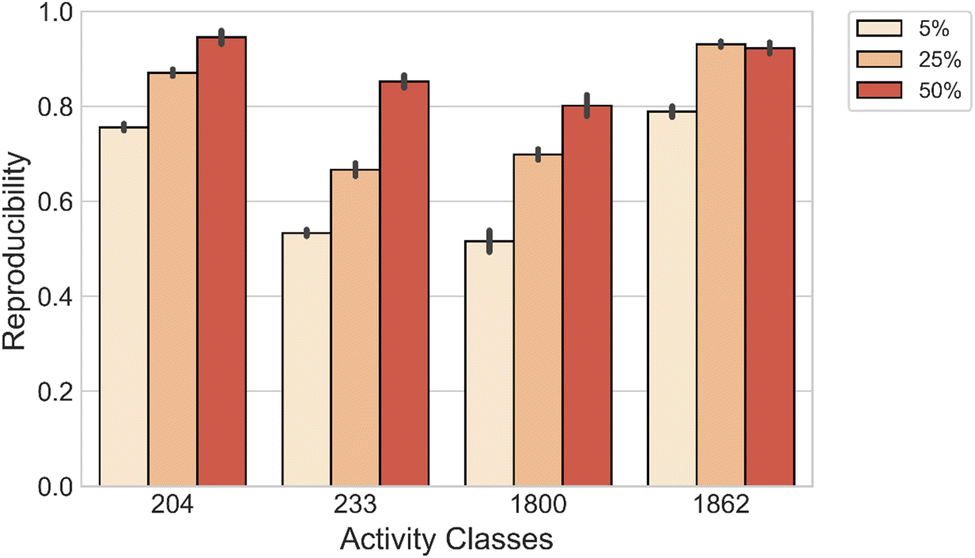Fig. 3 Reproducibility of MMP-Cliffs and MMP-nonCliffs originating from the same source compound.

3.4 Performance comparison of unconditional and conditional DeepAC

We also compared model performance of conditional DeepAC and unconditional DeepAC generated by randomly shuffling potency differences of MMPs during fine-tuning. Accordingly, for each activity class, potency differences were randomly shuffled for the three training set sizes (5, 25, and 50%) for the fine-tuning MMPs; then the pre-trained transformer was fine-tuned using these artificial MMPs. As shown in Fig. 4A, for MMP-Cliffs, the reproducibility of conditional DeepAC was significantly higher than of unconditional DeepAC. However, for the reproducibility of MMP-nonCliffs, conditional DeepAC only yielded slight improvement than unconditional DeepAC (Fig. 4B). This was principally expected because potency differences of most MMP-nonCliffs remained similar (less than one order of magnitude). These findings further demonstrated that potency difference of ACs played a critical role for model derivation.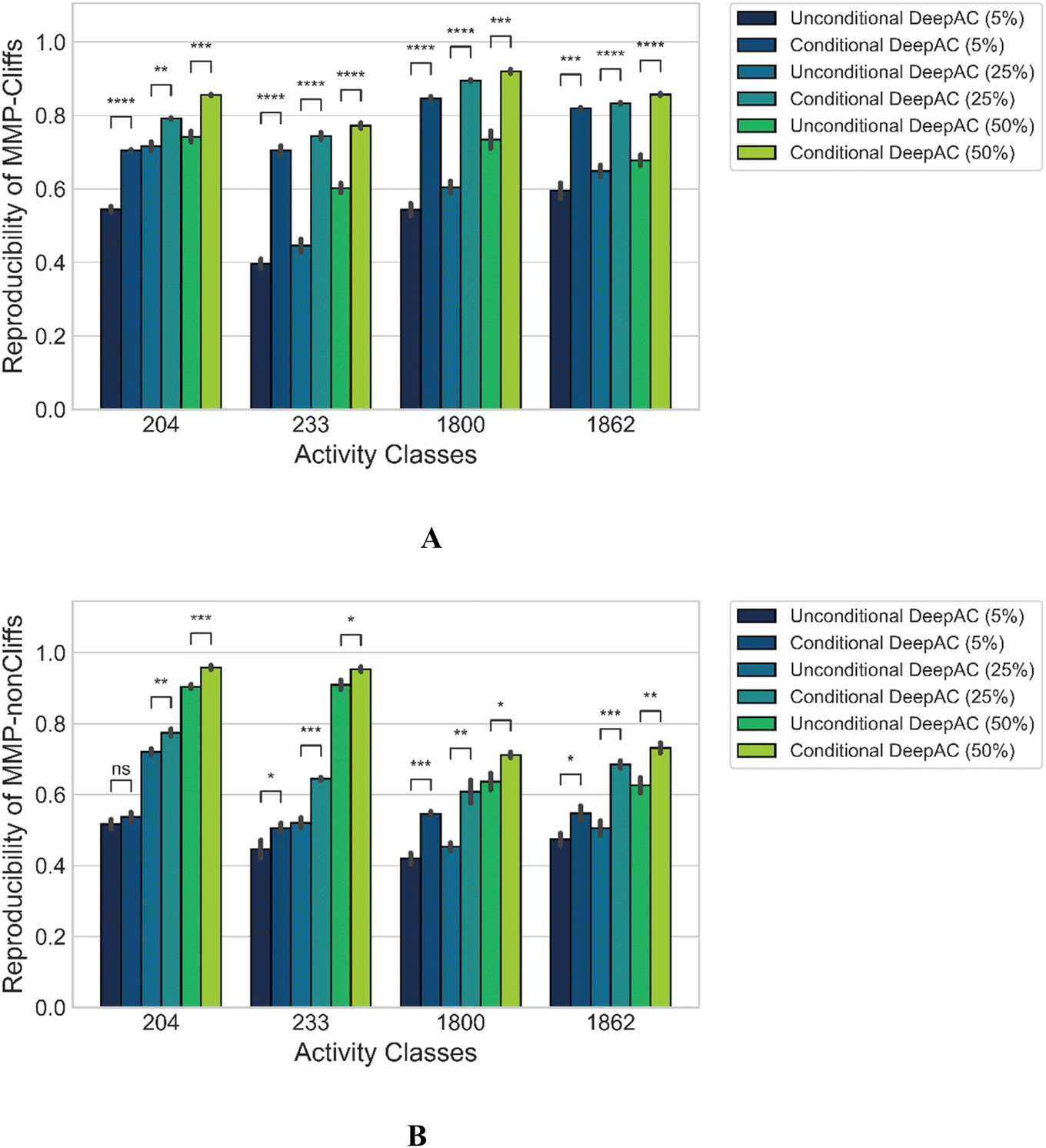

Fig. 4 Performance of conditional vs. unconditional DeepAC. Reproducibility is reported for (A) MMP-Cliffs and (B) MMP-nonCliffs. Mean and standard deviations (error bars) are provided for each activity class. Independent-samples t tests were conducted: 0.05 < p ≤ 1.00 (ns), 0.01 < p ≤ 0.05 (*), 0.001 < p ≤ 0.01 (**), 0.0001 < p ≤ 0.001 (***), p ≤ 0.0001 (****).

3.5 Alternative fine-tuning

As an additional control, fine-tuning was carried out using MMP-nonCliffs (ΔpK_i < 1.0) and MMPs with 1.0 ≤ ΔpK_i < 2.0 that were initially excluded from the analysis to prevent potential bias due to boundary effects. Then, the reproducibility of MMP-Cliffs of the fine-tuned models was determined and compared to regular fine-tuning. Fig. 5A shows that fine-tuning only with MMP-nonCliffs yielded reproducibility of 0.306–0.576 for the activity classes, reflecting a baseline learning effect of MMPs and associated potency differences, even if these were only small. However, fine-tuning with MMPs (1.0 ≤ ΔpK_i < 2.0), significantly increased the reproducibility of MMP-Cliffs to 0.620 for thrombin inhibitors, 0.607 for Mu opioid receptor ligands, 0.726 for corticotropin releasing factor receptor 1 ligands and 0.716 for tyrosine kinase Abl inhibitors. Fine-tuning using increasing proportions of MMP-Cliffs further increased reproducibility. Taken together, these findings clearly demonstrated the influence of MMP-associated potency differences for AC predictions. Furthermore, consistent with these observations, Fig. 5B shows that fine-tuning with MMP-nonCliffs, led to very high reproducibility of MMP-nonCliffs, which was substantially reduced when fine-tuning was carried out with MMPs capturing larger potency differences.

Fig. 5 Model performance comparison after alternative fine-tuning with different types of MMPs. Reproducibility of (A) MMP-Cliffs and (B) MMP-nonCliffs is reported. Mean and standard deviations (error bars) are provided for each activity class. Independent-samples t tests were conducted: 0.05 < p ≤ 1.00 (ns), 0.01 < p ≤ 0.05 (*), 0.001 < p ≤ 0.01 (**), 0.0001 < p ≤ 0.001 (***), p ≤ 0.0001 (****).

3.6 Global performance comparison

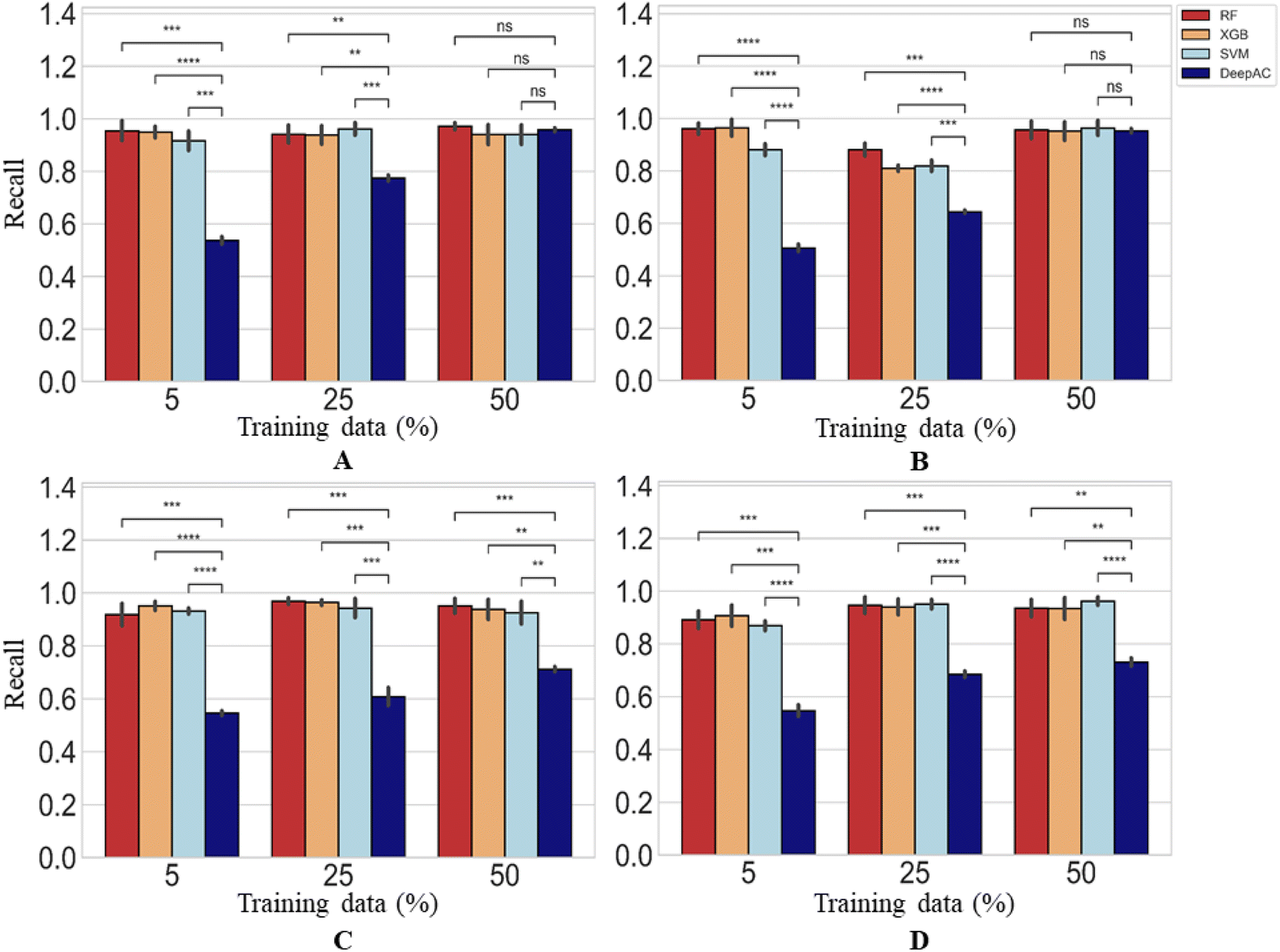
The performance of DeepAC in activity prediction was compared to other machine learning methods including SVM, RF, and XGboost. First, the reproducibility/recall of MMP-Cliffs and MMP-nonCliffs from the four activity classes was compared for unbalanced training and test sets according to Table 1. For AC prediction, unbalanced sets were deliberately used to account for the fact that ACs are rare compared to other pairs of structural analogues with minor potency differences, thus providing a realistic prediction scenario.

The predictions using different methods were generally stable, yielding only low standard deviations over independent trials (Fig. 6). Using 5% of training data for fine-tuning or model derivation, the recall (TPR) of MMP-Cliffs was consistently higher for DeepAC than the reference methods, which failed on two activity classes (Fig. 6). For increasing amounts of training data, recall performance of the reference methods further increased and SVM reached the 80% or 90% recall level of DeepAC in two cases when 50% of available data were used for training (Fig. 6).

Fig. 6 Recall of MMP-Cliffs. For four different methods, recall/reproducibility of MMP-Cliffs is reported for (A) thrombin inhibitors, (B) Mu opioid receptor ligands, (C) corticotropin releasing factor receptor 1 ligands, and (D) tyrosine kinase Abl inhibitors. Average recall over five independent trials is reported for increasing amounts of training data randomly selected from the complete data set (error bars indicate standard deviations). Statistical tests are shown according to Fig. 4.

For MMP-nonCliffs, representing the majority class for the predictions, a different picture was obtained. Here, the recall of reference methods for increasing amounts of training data was mostly greater than 90% and significantly higher than of DeepAC (Fig. 7). For DeepAC, recall/reproducibility increased with increasing amounts of training data and reached highest performance very similar to the reference methods for two activity classes when 50% training data were used.

Fig. 7 Reproducibility of MMP-nonCliffs. In (A)–(D), reproducibility of MMP-nonCliffs is reported using four different methods. Statistical tests are shown according to Fig. 4.

Calculation of BA for the prediction of MMP-Cliffs and MMP-nonCliffs gave similar results for all methods (Fig. 8). The level of 80% BA was generally reached for 25% or 50% training data. For largest training sets, all methods were comparably accurate for two activity classes, SVM reached highest accuracy for one class, and DeepAC for another (Fig. 8). Compared to the other methods, DeepAC produced higher TPR and lower TNR values, resulting in overall comparable BA. Clearly, a major strength of DeepAC was the ability to accurately predict MMP-Cliffs on the basis of small training data sets.

Fig. 8 Prediction accuracy. Reported are mean BA values and standard deviation (error bars) for the prediction of MMP-Cliffs and MMP-nonCliffs. In (A)–(D), results are reported using four different methods and statistical tests according to Fig. 4.

3.7 Activity cliff predictions in context

As discussed above, AC predictions have been reported previously in independent studies, which are summarized (and ordered chronologically) in Table 5. In 2012, AC predictions with SVM and newly designed MMP kernels yielded high accuracy,⁹ which was also achieved in several subsequent studies using modified SVM approaches (Table 5). In addition, in our current study, we have investigated decision tree methods for AC predictions using molecular representations adapted from SVM, which yielded comparably high accuracy. Hence, although AC predictions are principally challenging, for reasons discussed above, different machine learning methods have produced high-quality models for different compound data sets. Accordingly, there would be little incentive to investigate increasingly complex models for AC predictions. Nonetheless, recent studies have investigated deep learning approaches for AC predictions, with different specific aims. These investigations included the use of convolutional neural networks for predicting ACs from image data^14,15 and the use of graph neural networks for AC representation learning.¹⁶ While these studies provided proof-of-concept for the utility of novel methodologies for AC predictions, improvements in prediction accuracy compared to SVM in earlier studies have been marginal at best. The first eight studies in Table 5 report classification models of varying complexity for AC prediction. While most of these studies applied the MMP-Cliff formalism, their system set-ups, calculation conditions, and test cases differed such that prediction accuracies can only be globally compared and put into perspective including our current study. Furthermore, the last two studies^17,18 in Table 5 report regression models for potency prediction of individual AC compounds that are distinct from the others, precluding comparison of the results (these studies also used different AC definitions). However, they are included for completeness.

Table 5 Activity cliff predictions^a

Study	AC criteria, similarity/potency difference	Prediction task	Methods	Prediction accuracy
a Abbreviations: SVM/R (support vector machine/regression); F1 (mean F1 score); AUC (area under the ROC curve); MCC (Matthews' correlation coefficient); 3D-ACs (three-dimensional activity cliffs); VLS (virtual ligand screening); CGR (condensed graphs of reaction); CNN (convolutional neural network); MCS (maximum common substructure); RF (random forest); DNN (deep neural network); GCN (graph convolutional network); MPNN (message passing neural network); GAT (graph attention network); RMSE (root mean square error); KNN (K-nearest neighbor); GBM (gradient boosting machine); AFP (attentive fingerprint); LSTM (long short-term memory network).
Heikamp et al.^9	MMP/100-fold	ACs for 9 activity classes	Fingerprint-based SVM with MMP kernels	F1: 0.70–0.99
Husby et al.^13	Binding mode similarity (80%)/100-fold	3D-ACs for 9 activity classes	Docking/VLS	AUC: 0.75–0.97
Horvath et al.^10	MMP/100-fold	ACs for 7 activity classes	CGR and descriptor recombination-based SVM/SVR	F1: 0.61–0.92
Tamura et al.^12	MMP/100-fold	ACs for 9 activity classes	Fingerprint-based SVM with Tanimoto kernel	MCC: ∼0.20–0.80
Iqbal et al.^14	MMP/100-fold	ACs from MMP images and R-groups (5 activity classes)	Image-based CNN with transfer learning	F1: 0.28–0.76
				MCC: 0.24–0.73
Iqbal et al.^15	MMP/100-fold	ACs from MMP images (3 activity classes)	Image-based CNN	F1: 0.36–0.85
				AUC: 0.92–0.97
				MCC: 0.39–0.83
Tamura et al.^11	MMP/100-fold	ACs for 2 activity classes	Fingerprint-based SVM with MMP kernel	AUC: 0.46–0.69
				MCC: 0.69–0.89
Park et al.^16	MMP/100-fold	ACs for 3 activity classes	GCN	F1: 0.34–0.49
				AUC: 0.91–0.94
				MCC: 0.40–0.49
Jiménez-Luna et al.^17	MCS/10-fold	—	RF/DNN/GRAPHNET/GCN/MPNN/GAT	RMSE: 0.698–1.029
Tilborg et al.^18	Scaffold SMILES similarity (90%)/10-fold	ACs for 30 activity classes	KNN/RF/GBM/SVM/MPNN/GAT/GCN/AFP/LSTM/CNN/Transformer	RMSE: 0.62–1.60

---

With DeepAC, we have introduced the use of conditional chemical language models for AC prediction. Given that most studies in Table 5 reported F1 (ref. 38) and Matthews' correlation coefficient (MCC)³⁹ scores for evaluating prediction accuracies, we also calculated these scores for the DeepAC predictions reported herein. With F1 of 0.50–0.78 and MCC of 0.43–0.75, DeepAC also yielded state-of-the-art prediction accuracy (and higher accuracy than recent AC predictions using graph neural networks¹⁶). However, DeepAC is principally distinguished from other AC predictions approaches by its ability to generate new compounds meeting AC criteria, which partly motivated its development.

4 Conclusion

In this work, we have investigated chemical language models for predictive modeling of ACs, a topical issue in both chemical informatics and medicinal chemistry, with high potential for practical applications. ACs are rich in SAR information and represent focal points of compound optimization efforts. For chemical language models, an encoding strategy was devised to predict target compounds from source compounds and associated potency differences. Seq2Seq and transformer models were pre-trained on pairs of structural analogues with varying potency differences representing true SARs and compared, revealing superior performance of the transformer architecture in reproducing test compound pairs. The pre-trained transformer was then fine-tuned on ACs and non-ACs from different activity classes. It was conclusively shown that the transformer learned structural relationships in combination with associated potency differences and thus accounted for SARs. Compared to reference methods, the conditional transformer (DeepAC) reached state-of-the-art prediction accuracy but displayed different prediction characteristics. DeepAC was less effective in predicting non-ACs, but predicted ACs with higher accuracy than reference methods, especially on the basis of small training data sets. A unique feature of DeepAC is its ability to generate novel candidate compounds. This ability and the observed prediction characteristics render DeepAC attractive for practical applications aiming to generate new highly-potent AC compounds, which will be investigated in future studies.

Data availability

All calculations were carried out using publicly available programs, computational tools, and compound data. Python scripts used for implementing chemical language models and curated activity classes used for AC predictions are freely available via the following link: https://doi.org/10.5281/zenodo.7153115

Author contributions

All authors contributed to designing and conducting the study, analyzing the results, and preparing the manuscript.

Conflicts of interest

There are no conflicts of interest to declare.

Acknowledgements

H. C. is supported by the China Scholarship Council.

References

1. G. M. Maggiora, J. Chem. Inf. Model., 2006, 46, 1535.
2. D. Stumpfe, Y. Hu, D. Dimova and J. Bajorath, J. Med. Chem., 2014, 57, 18–28.
3. D. Stumpfe, H. Hu and J. Bajorath, ACS Omega, 2019, 4, 14360–14368.
4. D. R. Flower, J. Chem. Inf. Comput. Sci., 1998, 38, 379–386.
5. J. Hussain and C. Rea, J. Chem. Inf. Model., 2010, 50, 339–348.
6. H. Hu, D. Stumpfe and J. Bajorath, Future Med. Chem., 2019, 11, 379–394.
7. D. Stumpfe and J. Bajorath, Future Med. Chem., 2015, 7, 1565–1579.
8. R. Guha, J. Chem. Inf. Model., 2012, 2, 2181–2191.
9. K. Heikamp, X. Hu, A. Yan and J. Bajorath, J. Chem. Inf. Model., 2012, 52, 2354–2365.
10. D. Horvath, G. Marcou, A. Varnek, S. Kayastha, A. de la Vega de León and J. Bajorath, J. Chem. Inf. Model., 2016, 56, 1631–1640.
11. S. Tamura, S. Jasial, T. Miyao and K. Funatsu, Molecules, 2021, 26, 4916.
12. S. Tamura, T. Miyao and K. Funatsu, Mol. Inf., 2020, 39, 2000103.
13. J. Husby, G. Bottegoni, I. Kufareva, R. Abagyan and A. Cavalli, J. Chem. Inf. Model., 2015, 55, 1062–1076.
14. J. Iqbal, M. Vogt and J. Bajorath, Artif. Intell. Life Sci., 2021, 1, 100022.
15. J. Iqbal, M. Vogt and J. Bajorath, J. Comput.-Aided Mol. Des., 2021, 35, 1157–1164.
16. J. Park, G. Sung, S. Lee, S. Kang and C. Park, J. Chem. Inf. Model., 2022, 62, 2341–2351.
17. J. Jiménez-Luna, M. Skalic and N. Weskamp, J. Chem. Inf. Model., 2022, 62, 274–283.
18. D. van Tilborg, A. Alenicheva and F. Grisoni, Exposing the limitations of molecular machine learning with activity cliffs, ChemRxiv preprint, 2022.
19. A. Gaulton, A. Hersey, M. Nowotka, A. P. Bento, J. Chambers, D. Mendez, P. Mutowo, F. Atkinson, L. J. Bellis, E. Cibrián-Uhalte, M. Davies, N. Dedman, A. Karlsson, M. P. Magarinos, J. P. Overington, G. Papadatos, I. Smit and A. R. Leach, Nucleic Acids Res., 2017, 45, D945–D954.
20. D. Weininger, J. Chem. Inf. Comput. Sci., 1988, 28, 31–36.
21. X. Hu, Y. Hu, M. Vogt, D. Stumpfe and J. Bajorath, J. Chem. Inf. Model., 2012, 52, 1138–1145.
22. I. Sutskever, O. Vinyals and Q. V. Le, Adv. Neural Inf. Process. Syst., 2014, pp. 3104–3112.
23. J. He, H. You, E. Sandström, E. Nittinger, E. J. Bjerrum, C. Tyrchan, W. Czechtizky and O. Engkvist, J. Cheminf., 2021, 13, 1–7.
24. M.-T. Luong, H. Pham and C. D. Manning, Proceedings of the 2015 conference on empirical methods in natural language processing, 2015, pp. 1412–1421.
25. A. Vaswani, N. Shazeer, N. Parmar, J. Uszkoreit, L. Jones, A. N. Gomez, Ł. Kaiser and I. Polosukhin, Adv. Neural Inf. Process. Syst., 2017, pp. 5998–6008.
26. V. Nair and G. E. Hinton, ICML, 2010, pp. 807–814.
27. J. Ba, J. R. Kiros and G. E. Hinton, arXiv preprint arXiv:1607.06450, 2016.
28. K. He, X. Zhang, S. Ren and J. Sun, IEEE Conference on Computer Vision and Pattern Recognition (CVPR), 2015, pp. 770–778.
29. G. Landrum, RDkit: Open-source cheminformatics, 2006.
30. A. Aszke, S. Gross, F. Massa, A. Lerer, J. Bradbury, G. Chanan, T. Killeen, Z. Lin, N. Gimelshein, L. Antiga, A. Desmaison, A. Kopf, E. Yang, Z. DeVito, M. Raison, A. Tejani, S. Chilamkurthy, B. Steiner, L. Fang, J. Bai and S. Chintala, Adv. Neural Inf. Process. Syst., 2019, vol. 32, pp. 8026–8037.
31. V. N. Vapnik, The nature of statistical learning theory, Springer, New York, 2000.
32. L. Breiman, Mach. Learn., 2001, 45, 5–32.
33. T. Chen and C. Guestrin, Proceedings of the 22nd ACM SIGKDD International Conference on Knowledge Discovery and Data Mining, 2016, p. 785794.
34. F. Pedregosa, G. Varoquaux, A. Gramfort, V. Michel, B. Thirion, O. Grisel, M. Blondel, P. Prettenhofer, R. Weiss, V. Dubourg, J. Vanderplas, A. Passos, D. Cournapeau, M. Brucher, M. Perrot, E. Duchesnay and G. Louppe, J. Mach. Learn. Res., 2011, 12, 2825–2830.
35. D. Rogers and M. Hahn, J. Chem. Inf. Model., 2010, 50, 742–754.
36. J. Bergstra, B. Komer, C. Eliasmith, D. Yamins and D. Cox, Comput. Sci. Discovery, 2015, 8, 014008.
37. K. H. Brodersen, C. S. Ong, K. E. Stephan and J. M. Buhmann, Proceedings of the 20th International Conference on Pattern Recognition (ICPR), 2010, pp. 3121–3124.
38. C. J. Van Rijsbergen, Information retrieval, Butterworth-Heinemann, Oxford, 1979.
39. B. W. Matthews, Biochim. Biophys. Acta, Protein Struct., 1975, 405, 442–451.

---