
 Open Access Article
 This Open Access Article is licensed under a
 Creative Commons Attribution 3.0 Unported Licence
Database for liquid phase diffusion coefficients at infinite dilution at 298 K and matrix completion methods for their prediction†
Oliver
Großmann‡
 ,
Daniel
Bellaire‡
,
Nicolas
Hayer‡
,
Fabian
Jirasek
* and
Hans
Hasse
,
Daniel
Bellaire‡
,
Nicolas
Hayer‡
,
Fabian
Jirasek
* and
Hans
Hasse
Laboratory of Engineering Thermodynamics (LTD), TU Kaiserslautern, Erwin-Schrödinger-Straße 44, 67663 Kaiserslautern, Germany. E-mail: fabian.jirasek@mv.uni-kl.de
First published on 11th October 2022
Abstract
Experimental data on diffusion in binary liquid mixtures at 298 ± 1 K from the literature were systematically consolidated and used to determine diffusion coefficients D∞ij of solutes i at infinite dilution in solvents j in a consistent manner. The resulting database comprises basically all data on D∞ij at 298 K that are available and includes 353 points, covering 208 solutes and 51 solvents. In a first step, the new database was used to evaluate semiempirical methods for predicting D∞ij from the literature, namely the methods of Wilke and Chang, Reddy and Doraiswamy, Tyn and Calus, and SEGWE, of which SEGWE yielded the best results. Furthermore, a new method for the prediction of D∞ij based on the concept of matrix completion from machine learning was developed, which exploits the fact that experimental data for D∞ij can be represented as elements of a sparse matrix with rows and columns corresponding to the solutes i and solvents j; it is demonstrated that matrix completion methods (MCMs) can be used for closing the gaps in this matrix. Three variants of this approach were studied here, a purely data-driven MCM and two hybrid MCMs, which use information from SEGWE together with the experimental data. The methods were evaluated using the new database. The hybrid MCMs outperform both the data-driven MCM and all established semiempirical models in terms of predictive accuracy.
1 Introduction
Diffusion plays a central role in many processes in nature and industry. Despite this, experimental data on diffusion coefficients are astonishingly scarce. In the present work, we address this topic for diffusion coefficients of a solute i highly diluted in a solvent j, which are particularly important both for practical and theoretical reasons, by setting up the first comprehensive database for diffusion coefficients at infinite dilution and the development of novel methods for their prediction.In general, mutual diffusion must be distinguished from self-diffusion. Mutual diffusion refers to the motion of collectives of molecules of different components in a mixture, and is directly relevant for describing technical processes. Self-diffusion, on the other hand, refers to the Brownian motion of individual molecules, and is defined for pure components as well as for mixtures.
There are two common approaches for describing mutual diffusion: the Fickian and the Maxwell–Stefan approach. We study only binary mixtures here, so that the following discussion is limited to this case. The Fickian diffusion coefficient Dij and the Maxwell–Stefan diffusion coefficient Đij in a binary mixture (i + j) are related by eqn (1):
| Dij = ĐijΓij, | (1) |
| D∞ij = Đ∞ij = D∞i. | (2) |
Information on D∞ij is directly relevant in problems in which the diffusing component is diluted. Furthermore, there are methods to estimate Đij at finite concentrations from the respective values at infinite dilution, i.e., of Đ∞ij and Đ∞ji, most notably that of Vignes1 for binary mixtures, which has also been extended to multicomponent mixtures where experimental data on diffusion coefficients are lacking almost completely.2
Experimental data on diffusion coefficients have been compiled in several databases. For instance, in the 2019 version of the Dortmund Data Bank (DDB), which is the worlds largest data bank for thermophysical properties of pure components and mixtures, approximately 17![[thin space (1/6-em)]](https://www.rsc.org/images/entities/char_2009.gif) 000 data points for diffusion coefficients are reported.3 These data points cover approximately 580 individual components and 1300 distinct mixtures, of which about 75% are binary mixtures. These data include diffusion coefficients of different types for the gaseous, liquid, and solid phase, measured at different compositions, temperatures and pressures. Compared to the number of relevant components and, in particular, mixtures, the experimental database on diffusion coefficients is very small. While this holds basically for all thermophysical properties, the situation for diffusion coefficients is even worse than that for other properties, such as activity coefficients,4 which is astonishing regarding the importance of diffusion. This could be related to the challenges in measuring diffusion coefficients.5 Therefore, methods for the prediction of diffusion coefficients in general, and D∞ij in particular, are of paramount importance in practice.
000 data points for diffusion coefficients are reported.3 These data points cover approximately 580 individual components and 1300 distinct mixtures, of which about 75% are binary mixtures. These data include diffusion coefficients of different types for the gaseous, liquid, and solid phase, measured at different compositions, temperatures and pressures. Compared to the number of relevant components and, in particular, mixtures, the experimental database on diffusion coefficients is very small. While this holds basically for all thermophysical properties, the situation for diffusion coefficients is even worse than that for other properties, such as activity coefficients,4 which is astonishing regarding the importance of diffusion. This could be related to the challenges in measuring diffusion coefficients.5 Therefore, methods for the prediction of diffusion coefficients in general, and D∞ij in particular, are of paramount importance in practice.
Several correlations for the prediction of D∞ij in binary liquid mixtures have been proposed in the literature,6 of which the most commonly used ones are those of Wilke and Chang (1955), Reddy and Doraiswamy (1967), Tyn and Calus (1975), and the Stokes–Einstein Gierer–Wirtz Estimation (SEGWE) of Evans at al. (2018).7–10 They are all empirical extensions of the Stokes–Einstein equation11 and may therefore be classed as semiempirical models.
A large number of further semiempirical models for the prediction of D∞ij in binary liquid mixtures or extensions upon the previously mentioned ones exist in the literature, but most of them are either less general (in the scope of the components that can be modeled by them) or less accurate than these.12 Power-law models, which have also been applied in the literature for modeling diffusion coefficients,13–15 suffer from a similar restriction in generality as they must be “calibrated” to a specific substance group, and they depend strongly on the type of components investigated. For a more detailed discussion of such approaches and their delimitation from the semiempirical models investigated here, we refer to the review of Evans.16
As an alternative to physical and semiempirical prediction methods for thermophysical properties in general, data-driven approaches from machine learning (ML) are presently gaining much attention.17–20 In most of the respective works, ML algorithms are thereby used for correlating thermophysical properties of pure components to a set of selected pure-component descriptors in a supervised manner. As such, most of these approaches can be classified as quantitative structure–property relationships (QSPR).21
Descriptor-based methods of the QSPR type can also be used for predicting mixture properties, and of course also for the prediction of diffusion coefficients. In particular, artificial neural networks (ANNs) have been used successfully in QSPR approaches by several authors,22–25 however, these studies were often restricted to specific mixtures, such as diffusion in water24,25 or diffusion in hydrocarbon mixtures;22 general-purpose models for the prediction of diffusion coefficients at infinite dilution based on ML methods are still missing to date.
An interesting class of unsupervised ML algorithms for the prediction of thermophysical properties of mixtures in general, and of D∞ij in particular, are matrix completion methods (MCMs), which are already established in recommender systems, e.g., for providing suitable movie recommendations to customers of streaming providers.26,27
The idea behind using MCMs for predicting thermophysical properties of mixtures is that the data for binary mixtures can, at constant conditions, be stored in matrices with rows and columns representing the components that make up the mixtures; since these matrices are only sparsely occupied by experimental data in basically all cases, the prediction of the properties of unstudied mixtures can be regarded as a matrix completion problem. The MCM algorithms solve this problem by learning similarities between different rows and columns, i.e., the different instances, and using the inferred knowledge for predicting the missing entries. Obviously, this requires a certain amount of data for the learning step and becomes the more challenging the sparser the matrix is occupied and the weaker the correlations between the entries in the columns and rows are.28 The relevance of MCMs for predicting thermophysical properties of binary mixtures has only been realized recently.4,17 In particular, they have been applied very successfully for predicting activity coefficients and Henry's law constants.4,28–31 In the present work, we extend the MCM approach to the prediction of diffusion coefficients.
The contribution of the present work is threefold. Firstly, we have established a consolidated, consistent database of liquid phase diffusion coefficients at infinite dilution D∞ij in binary mixtures at 298.15 ± 1 K based on a careful evaluation of the literature data. We have mainly used data from the Dortmund Data Bank (DDB).3 In many cases, this required extrapolations of data at finite concentration to infinite dilution, which we have carried out in a consistent manner for the first time. Furthermore, the data from DDB were consolidated and augmented by data sets from the literature that were not included in the DDB. The results can be represented in an m × n matrix, in which the rows represent the solutes (m = 208) and the columns represent the solvents (n = 51). However, only 353 of the 10608 elements of that matrix are occupied with experimental data, corresponding to 3.3%. For the rest, experimental data are missing.
Second, we have used the new database to systematically evaluate the performance of four widely applied semiempirical methods for the prediction of D∞ij, namely those of Wilke and Chang,7 Reddy and Doraiswamy,8 Tyn and Calus,9 and SEGWE.10
Third, we have developed a data-driven MCM for the prediction of D∞ij, which is trained only on the few available experimental data points on D∞ij from our database, as well as two hybrid MCMs that combine the semiempirical SEGWE with the data-driven MCM in different ways. All MCMs presented in this work are collaborative-filtering approaches that learn only from the available data for the mixture property D∞ij, but do not require information on additional descriptors of the solutes and solvents, which is in contrast to supervised QSPR methods.32 The predictions of the MCMs were compared to each other and to the results from the established semiempirical models.
2 Database
Raw diffusion data was mainly taken from the Dortmund Data Bank (DDB) 2019.3Fig. 1 shows a classification of the 17085 data points on diffusion coefficients available in the DDB. Approximately 75% (12869) of these data points are reported for binary mixtures, of which about 60% consider diffusion in the liquid phase and are of interest here.
 | ||
| Fig. 1 Sankey diagram representing the different types of data on diffusion coefficients in the Dortmund Data Bank (DDB) 2019, including information on the number of available data points.3 The red branches lead to the data considered in the present work. | ||
We have restricted this study to well-defined molecular components, i.e., we have excluded mixtures that contain polymers or pseudocomponents as well as some other special cases (cf. ESI Section S.1†). We will not continue to mention these restrictions in the following discussion.
Fig. 2 shows a histogram representation of all data points in the DDB that comply with the selection criteria over the temperature at which they were measured. About 30% of the data points (2064) were measured in the range 298.15 ± 1 K, which is why we have selected this temperature for our study, in which we only wanted to consider isothermal data.
 | ||
| Fig. 2 Histogram representing the number of experimental data points for diffusion coefficients in binary liquid mixtures from the DDB meeting the selection criteria illustrated in Fig. 1 as a function of the temperature T. | ||
Of these 2064 data points, only a small fraction (13%) is reported as diffusion coefficients at infinite dilution D∞ij, while most reported data points are concentration-dependent Dij(x), cf. also Fig. 1. For setting up the database on D∞ij, the following procedure was applied:
First, the data points for D∞ij from the DDB were adopted; in cases in which data from several sources were available for the same mixture, the arithmetic mean was used. Second, concentration-dependent Dij(x) were extrapolated to the state of infinite dilution. For this, all data points at solute concentrations xi above 0.2 mol mol−1 were discarded. Then, depending on the number of remaining data points Nij for a specific mixture i + j, the following heuristics were applied:
(a) Nij = 1: the reported value of Dij was adopted if the solute concentration xi was below 0.02 mol mol−1, otherwise it was discarded.
(b) Nij = 2: D∞ij was obtained from a linear extrapolation of the two data points to xi = 0.
(c) Nij ≥ 3: D∞ij was calculated by linear extrapolation to xi = 0, starting with the points at the lowest concentrations and including as many points as possible before a discernible deterioration in fit quality was observed.
For each of the cases (a)–(c) detailed above, an example of the performed extrapolation is given in Fig. 3. This procedure was selected after considering a large number of binary mixtures and testing alternatives. We have preferred applying a standard procedure over an ad hoc consideration of each mixture, not only because of the time required for this but also to avoid ambiguity. In all cases, obvious outliers were rejected beforehand (cf. ESI Section S.1†).
 | ||
| Fig. 3 Procedure of determining D∞ij. (a) The single value for Dij(x) reported at xi = 0.02 mol mol−1 was adopted as D∞ij. (b) The two values for Dij(x) reported at xi < 0.2 mol mol−1 were linearly extrapolated to D∞ij. (c) The three values for Dij(x) with the lowest xi, all at xi < 0.2 mol mol−1, were included in the linear extrapolation to D∞ij. Blue open circles: literature data.3 Red closed circles: extrapolated D∞ij. Lines: linear extrapolations. | ||
As many data points were simply adopted, it is difficult to give an estimate for the uncertainty of the data: many literature sources do not report uncertainties for the measured diffusion coefficients, and those who do typically specify uncertainties in the range of 1–5%. This seems over-optimistic, as in the few cases where direct comparisons between results from different sources were possible, deviations often were in the range of 10%. The errors induced by our extrapolation scheme are lower than the uncertainties mentioned above in all cases.
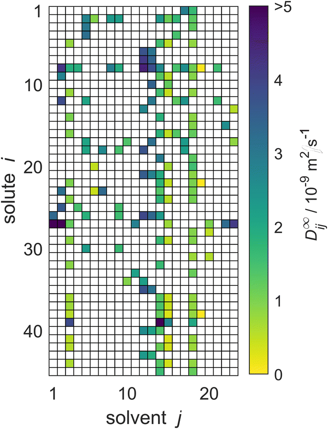
As result of this procedure, a database on D∞ij containing 353 data points for 208 solutes i and 51 solvents j was obtained. The database is represented in Fig. 4 in matrix form, where the rows represent the solutes i and the columns represent solvents j, both of which are simply identified by numbers. The value for D∞ij is indicated by the color of the respective matrix entry. The order of the solutes and solvents does not have a meaning but was chosen to be ascending with regard to the DDB identification numbers; Table S.1 in the ESI† gives a list with the names of all considered solutes and solvents and their identification numbers. In Table S.4,† the numerical values for D∞ij from the new database are given. The values are censored in instances where they have been directly adopted from the DDB and licensing restrictions prohibit their publication. Further, both tables are also provided in machine-readable form, namely as .csv files, in the ESI.†
 | ||
| Fig. 4 Overview of the experimental data for liquid phase diffusion coefficients D∞ij of solutes i in solvents j at infinite dilution at 298.15 ± 1 K in the database set up in the present work. Solutes and solvents are simply identified by numbers, see Table S.1 in the ESI.† The color code indicates the value of D∞ij, and white cells denote missing data. | ||
To the best of our knowledge, our database is the first comprehensive database of diffusion coefficients at infinite dilution. However, of the 10608 different possible combinations of the considered solutes and solvents, data are available only for 353 (3.3%). Furthermore, the resulting matrix is not only sparsely but also heterogeneously filled with observed entries, cf.Fig. 4; for instance, for the solvent water (column 28), a very large number of data points (with different solutes) is available, whereas many other solvents (and solutes) have been studied in only a very limited number of mixtures. In fact, a substantial share of the solutes that were studied in combination with water have not been studied in combination with any other solvent with regard to D∞ij.
3 Prediction of diffusion coefficients
3.1 Semiempirical models
The new database was used for studying the performance of four established semiempirical models for the prediction of D∞ij, namely those of Wilke and Chang (1955),7 Reddy and Doraiswamy (1967),8 Tyn and Calus (1975),9 and the Stokes–Einstein Gierer–Wirtz Estimation (SEGWE) by Evans et al. (2018).10 All considered models have in common that they predict D∞ij as a function of the quotient T/ηj, where T is the temperature in Kelvin and ηj is the dynamic viscosity of the solvent j. Hence, information of ηj at the temperature of interest is required. Furthermore, they all require information on the pure solute i, namely either the molar volume vi, the molar mass Mi, or the parachor Pi – or some combination thereof. All pure-component properties were obtained in the present work from DIPPR correlations taken from the DIPPR database.33 The Wilke–Chang and SEGWE models additionally require solvent-specific parameters. The authors provide some values of these parameters in the original publications, but in practice the parameters are typically first fitted to experimental data on D∞ij in the respective solvent j.For the comparison of the semiempirical models with the MCMs, we have fitted the solvent-specific parameters of Wilke–Chang and SEGWE to data on D∞ij from the new database using a leave-one-out procedure (cf. Section 3.2.4). This procedure ensures a fair comparison between the semiempirical models and the MCMs. However, when we used SEGWE as prior information for the hybrid MCMs, the parameter was not fitted, but instead a fixed global value was used. More information on the hybridization of SEGWE and MCM is given in Sections 3.2.2 and 3.2.3.
Furthermore, details on the semiempirical models are provided in Section S.2 of the ESI.†
3.2 Matrix completion methods
Three different MCMs were developed and evaluated in the present work: one MCM that is purely data-driven, i.e., which is only trained on the available experimental data for D∞ij from the new database. Furthermore, two hybrid MCMs, which additionally incorporate information from the SEGWE model in different ways as described below. In the following, we first discuss the general approach, matrix completion, and subsequently go into detail on each of the three individual MCMs.The underlying idea of the MCMs used in the present work is based on uncovering structure in a sparse matrix of data points Mij. An MCM thereby models each Mij as the dot product of two vectors ui and vj, in which so-called latent features of the pure solute i and the pure solvent j, respectively, are stored:
| Mij = ui·vj + εij | (3) |
Note that the latent features ui and vj are pure-component descriptors of i and j, respectively, which are inferred from mixture data. For training all MCMs, we followed a Bayesian approach, in which data and features are considered as random variables that follow a probability distribution. Therefore, a probabilistic generative model of the observations (here: Mij) as a function of ui and vj was specified based on eqn (3). More specifically, the probabilistic model was defined by the so-called prior, which represents the probability of the features prior to fitting them to the training data, and the so-called likelihood, which models the probability of the data on Mij conditioned on the model parameters. The goal of Bayesian inference is to find the so-called posterior, which is the probability distribution over model parameters conditioned on the training data, and which is consistent with the training data and the a priori information on the model parameters.34
While different priors were chosen in the different MCMs, the same likelihood in form of a Cauchy distribution with scale λ = 0.2 centered around the dot product ui ·vj was chosen for all MCMs. The Cauchy distribution was preferred over, e.g., a normal distribution since the Cauchy distribution is generally more robust towards outliers, which must be expected if experimental data are considered. Both the form of the prior and the likelihood, including the scale parameter λ, are hyperparameters of the model. In preliminary studies with different configurations, the hyperparameter set from our previous work31 proved to be most suitable, which was therefore adopted here. All feature vectors are of length K, where K is the number of features considered for each solute and each solvent. K is a further hyperparameter of the model and is a priori unknown; it must be chosen so that over- and underfitting are avoided. In preliminary studies, K = 2 was found the most suitable choice and was therefore used for all models here.
Since exact Bayesian inference is usually intractable, except for very simple models, methods for approximating the posterior are generally used in practice. In the present work, we have used variational inference for this purpose, which has been successfully applied to various models up to large scales.35–37 Specifically, we have employed Gaussian mean-field variational inference using the Automatic Differentiation Variational Inference (ADVI)37 option implemented in the probabilistic programming framework Stan,38 which was used for training all models. The code is attached in Section S.7 of the ESI.†
D∞ij is thereby modeled as the dot product of the two latent feature vectors ui and vj:| lnD∞ij = ui·vj + εij. | (4) |
 as the natural logarithm of the numerical value of the diffusion coefficient in 10−9 m2 s−1, which is used for scaling purposes.
During the training of the MCM, the generative model first draws two vectors ui and vj of length K with features for each solute i and solvent j from the prior, for which a normal distribution centered around zero with a standard deviation σ0 = 1 was chosen here. It then models the probability of each experimental data point lnD∞ij as a Cauchy distribution with scale λ centered around the dot product of the respective feature vectors, cf.eqn (4), and thereby adjusts the features so that they are best suited for describing the training data, i.e., minimizing the εij. When performing Bayesian inference, the probabilistic model is thereby inverted to obtain the posterior, i.e., the probability distribution over the features after considering the training data. The final features of the solutes and solvents were then obtained by taking the mean of the posterior, which we have subsequently used for calculating predictions for lnD∞ij with eqn (4) (while setting εij to zero).
D∞ij), but on the residuals resij of the SEGWE model:| resij = lnD∞,SEGWEij − lnD∞,expij = ui·vj. | (5) |
Hence, in this case, the MCM is not employed to uncover structure in the experimental data, but in the deviations of the SEGWE predictions from the experimental data.
For the Boosting approach, SEGWE was applied in a purely predictive manner; this means that the parameter ϱeff, cf. eqn (S.5),† was not treated as a fit parameter but globally set to the value ϱeff = 619 kg m−3 as suggested by the original authors.10
We have chosen SEGWE for the Boosting approach for two reasons: first, SEGWE proved to be the best-performing of the studied semiempirical models, cf. Section 4.1. Second, in the chosen variant of SEGWE, the only component descriptors required in the model equation are the viscosity of the solvent and the molar masses of solute and solvent; information on these properties is readily available.
The training of this hybrid MCM was carried out analogously to the data-driven approach and with the same hyperparameters (prior and likelihood as well as number of features per solute/solvent K). After the training, MCM-Boosting yields predictions of the residuals of the SEGWE model for specified mixtures (i + j). The respective predicted lnD∞ij (and thus D∞ij) can then be calculated from the predicted residuals by rearranging eqn (5).
The training of the Whisky model consists of two steps. In the first training step, the predictions of lnD∞ij obtained with SEGWE (again with globally fixed ϱeff = 619 kg m−3) for all combinations of the considered solutes and solvents were used for training a data-driven MCM according to eqn (4) (while again using the same hyperparameters as in the MCMs described above). As result, preliminary feature vectors  and
and  of the solutes i and solvents j, respectively, were obtained. We can interpret this training step as distilling the essence of the SEGWE model and storing it in the preliminary feature vectors
  and
and  ; we therefore call this first training step distillation step in the following.
In the second training step, the preliminary feature vectors  and
and  were refined using the (sparse) experimental data on D∞ij from our database; we therefore call the second training step maturation step in the following. In the maturation step, the preliminary
  and
and  were used for creating an informed prior for the training of an additional MCM, which was then trained on the experimental D∞ij. Specifically, the means of the respective preliminary features were adopted, whereas the standard deviations of the features were scaled with a constant factor, such that the mean of all resulting standard deviations was σ = 0.5. This scaling procedure was carried out analogously to our previous work31 and ensures that the model remains flexible enough to reasonably consider the experimental training data. The final informative prior for the maturation step of the hybrid MCM was then obtained by multiplying the scaled posterior from the distillation step with the uninformed prior distribution as used in the data-driven MCM. With this last step, we ensure that the informed prior is in all cases stronger than the uninformed prior.
Hence, in this hybrid MCM, information from SEGWE is included and transferred via the prior in the maturation step. However, the model is still capable of overruling the prior information from SEGWE via the likelihood, if the available experimental data for D∞ij is convincing enough to do so.
In both training steps of the Whisky model, the same likelihood (Cauchy with scale parameter λ = 0.2) and the same number of features per solute and solvent (K = 2) as in the other MCMs were used.
While both hybrid approaches, MCM-Boosting and MCM-Whisky, incorporate information from the SEGWE model, the difference is how the knowledge from the semiempirical model is encoded in the MCM as described above. MCM-Boosting can only lead to improvements over the baseline model (here: SEGWE) if that model shows systematic prediction errors. Only then can the MCM reveal structure in the residuals of the model and thereby refine the predictions. Furthermore, any information from SEGWE for mixtures for which no experimental data are available is inevitably discarded in the Boosting approach. In the Whisky approach, in contrast, different classes of training data are combined: predictions with the SEGWE model, which can be obtained for many mixtures (for the present data set, they could be obtained for all combinations of solutes and solvents) but rather uncertain, and experimental data, which are rare (cf. Section 2) but more reliable than model predictions. For components for which there are many experimental data, the Whisky approach can be expected to hardly improve the predictive performance compared to a data-driven MCM. On the other hand, for components for which there are only few experimental data for training, the largest improvements compared to the data-driven MCM can be expected with the Whisky approach.
By nature, such a leave-one-out analysis of an MCM demands a database in which at least two distinct data points are available for each solute i and each solvent j, so that after declaring one of these data points as test data point, there is at least one data point for each component in the training set to allow the model to learn its characteristics. Hence, if the database is arranged in matrix form with solutes and solvents representing the rows and columns, respectively, at least two observed entries per row and per column are required for a meaningful analysis.
Therefore, for developing the MCMs, a reduced database for D∞ij that satisfies the aforementioned condition was defined. To enable a direct comparison, the predictive performance of the semiempirical models was also evaluated based on this reduced data set. Thereby, the solvent-specific parameters of the models of Wilke and Chang and SEGWE were also fitted to experimental data for D∞ij in a leave-one-out approach (cf. Section S.2.5 of the ESI†).
The reduced database is presented in Fig. 5. It is the basis for the comparison of the performance of the three MCMs and the semiempirical models for predicting D∞ij considered in the present work.
 | ||
| Fig. 5 Overview of the experimental data for the liquid phase diffusion coefficients D∞ij at infinite dilution at 298.15 ± 1 K in the reduced database; these data points were used for evaluation of the MCMs developed in the present work and comparison of the results to those of the semiempirical models. Solutes and solvents are identified by numbers, see Tables S.2 and S.3 in the ESI.† The color code indicates the value of D∞ij, and white cells denote missing data. | ||
While the MCM only works for mixtures within the matrix shown in Fig. 5, the semiempirical models can also give predictions for additional mixtures outside the matrix, namely for all mixtures for which the required pure-component properties are known.
The reduced database comprises data for 45 solutes and 23 solvents. The corresponding matrix, which is shown in Fig. 5, has about 16% observed entries: for 166 of the 1035 possible mixtures experimental data are available.
Four particularly well-filled columns can be discerned for j = 3, 14, 15, and 18. The respective solvents are ethanol, methanol, n-propanol, and water. They are common solvents for which experimental data were measured in combination with many solutes. Moreover, a column-based structure can be observed in the absolute values of D∞ij themselves (and not just in the availability of data): for example, the diffusion coefficients in the solvent methanol (j = 14) are consistently higher than the respective diffusion coefficients in the solvent n-propanol (j = 15), which is readily seen by the darker colors in that column in Fig. 5. Two further solvents, n-hexane and n-heptane (j = 12 and j = 13, respectively), exhibit even darker colors, corresponding to even higher values of D∞ij. Similar structural relationships in the matrix exist also for the rows, e.g., for carbon dioxide (i = 39) comparatively large diffusion coefficients are found. We will show below that the MCMs developed in the present work are able to pick up on these relationships, and even identify more complex relationships in the data structure, which are veiled before the human eye.
The predictive performance of the methods was analyzed and compared in terms of a relative mean absolute error (rMAE), cf.eqn (6), and a relative root mean-squared error (rRMSE), cf.eqn (7), which were calculated by comparing the predictions (pred) obtained during the leave-one-out analysis to the respective experimental data (exp):
 | (6) |
 | (7) |
4 Results and discussion
In Fig. 6, the performance of the four studied semiempirical models, as well as that of the three developed MCMs for the prediction of the D∞ij from our reduced database, are compared in terms of the relative mean absolute error (rMAE) and the relative root mean-squared error (rRMSE), cf. Section 3.2.4.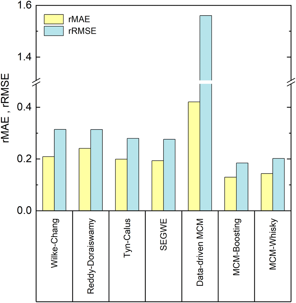 | ||
| Fig. 6 Relative mean absolute error (rMAE, yellow) and relative root mean-squared error (rRMSE, blue) of the predicted D∞ij with the studied semiempirical models and the developed MCMs for the experimental data from the reduced database. | ||
4.1 Prediction of D∞ij with semiempirical models
Let us first compare the results of the four semiempirical models.We observe a similar performance of all semiempirical models in both error metrics. The rMAE is about 0.20, and below 0.25 in all cases, with the largest value (poorest performance) found for the model of Reddy and Doraiswamy and the lowest value (best performance) found for SEGWE. Also, the values for the rRMSE vary only slightly between the different models and range from 0.31 (Reddy–Doraiswamy) to 0.28 (SEGWE). Although the four semiempirical models do not vary substantially in their rRMSE scores, we can observe a continuously decreasing rRMSE with the year of publication of the respective model. We can speculate that this is an effect of the increasing availability of experimental data, to which these models were fitted.
It is also important to note that, at the time these works were published, the authors presumably used the entirety of available data on D∞ij for developing their models. This means that the semiempirical models have already seen substantial parts of the data on which we evaluate their performance.
Comparing the rMAE and the rRMSE from the semiempirical models directly with the corresponding values from the MCM models, as it is done in Fig. 6, therefore creates a bias, which favors the semiempirical models; the calculation of the rMAE and rRMSE for the MCM models, in contrast, is based on a strict application of the leave-one-out strategy, i.e., none of the predicted values were part of the training set, which is not the case for the development of the semiempirical models. The fact that the fitting of solute-specific model parameters (of Wilke–Chang and SEGWE) was carried out with a leave-one-out technique does not change the above statement, as the model development was nonetheless based on all available data at that time.
Overall, SEGWE shows the best performance of the studied semiempirical models in both rMAE and rRMSE, and was therefore considered as benchmark against which the MCMs developed in the present work are compared in the following.
4.2 Prediction of D∞ij with matrix completion methods
We now discuss the performance of the MCMs for the prediction of D∞ij developed in this work: the purely data-driven MCM and the hybrid approaches based on Boosting, which we call MCM-Boosting, and the one based on model distillation, which we call MCM-Whisky in the following.The rMAE and rRMSE scores of the data-driven MCM are 0.42 and 1.56, respectively, which is much higher than those of all studied semiempirical models, cf.Fig. 6. The data-driven MCM thereby strongly suffers from a poor prediction of D∞ij in mixtures with the solvent 1,2-propanediol; namely the D∞ij in the mixtures (benzene + 1,2-propanediol) and (1,3-dihydroxybenzene + 1,2-propanediol) are predicted with extremely large relative errors of 1397% and 1339%, respectively, which results in a large rMAE and a particularly large rRMSE score for the data-driven MCM. As shown in Fig. 5, the experimental D∞ij for the solvent 1,2-propanediol (j = 19) are extremely small, namely about two orders of magnitude lower than the bulk of the data. Hence, already small absolute deviations between prediction and experimental D∞ij lead to extremely large errors on the relative scale, i.e., large values of rMAE and rRMSE, here. Excluding just the two mentioned data points from the evaluation improves the score of the data-driven MCM to 0.26 (vs. 0.42 with the points included) in the rMAE and 0.42 (vs. 1.56 with the points included) in the rRMSE – still slightly worse, but in the same range as the performance of the semiempirical methods.
An important requirement for the success of data-driven prediction methods in general, and the introduced data-driven MCM here in particular, is the availability of training data. One way to evaluate the data situation is comparing the number of available data points for training the model to the number of model parameters, which, among others, depends on the number of different components considered by the model. We can therefore assess an observation ratio 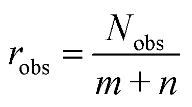 as done in recent work of our group,28 where Nobs is the number of observed entries of the sparsely populated matrix and m and n are the numbers of rows and columns of the matrix, i.e., considered solutes and solvents, respectively.
In our previous work, we found a strong correlation of the predictive performance of MCMs for the prediction of activity coefficients at infinite dilution with robs, which was between 4.4 and 9.2 in that study.28 Rather high values of robs led to a significantly better performance than rather low values. In the present study, the value of robs is 2.4, which is substantially smaller than the lowest studied value in ref. 28. This indicates that the situation regarding availability of training data is highly challenging here, in particular for the data-driven MCM, which leaves ample room for improvements. We only note here that also other points besides the mere number of training data points are important, like the heterogeneity in the number of available data for different components.
Such improvements can, as shown in Fig. 6, be achieved by hybridizing the data-driven MCM with information from SEGWE: both hybrid MCMs perform significantly better than all established semiempirical models and the data-driven MCM in both error scores rMAE and rRMSE. Let us first discuss the results of MCM-Boosting.
The key idea of MCM-Boosting is to train the algorithm on the residuals of the SEGWE model, and not on experimental data directly, cf. Section 3.2.2. In Fig. 7, the residuals between the SEGWE predictions and the data from our reduced database, cf.eqn (5), are plotted. Here, SEGWE was applied in the purely predictive variant with a globally fixed ϱ = 619 kg m−3 to ensure that no information on the test data point was included in the training of MCM-Boosting. Fig. 7 basically shows the performance of SEGWE for each individual data point from our reduced database. We observe large deviations, indicated by the color code in Fig. 7, in particular for the solutes water (i = 27) and carbon dioxide (i = 39), but beyond that, no apparent structure in the residuals is immediately recognizable. A more detailed discussion of the mixtures for which SEGWE gives predictions with particularly large errors is included in the ESI (cf. Section S.2.6†).
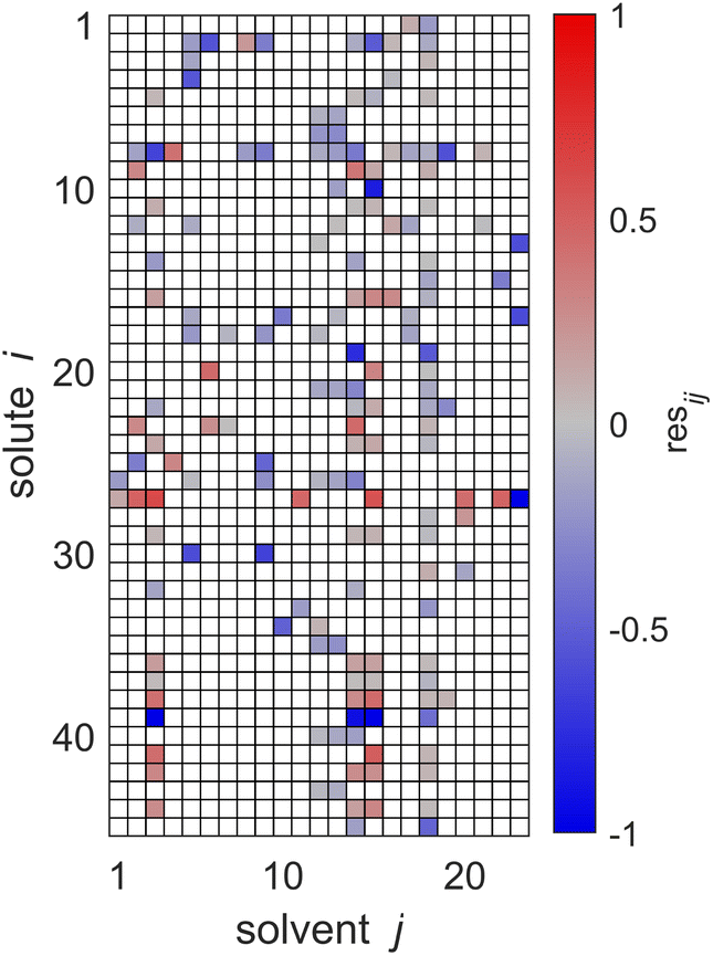 | ||
| Fig. 7 Residuals resij of the SEGWE predictions from the experimental data for D∞ij at 298.15 ± 1 K from our reduced database. Solutes i and solvents j are identified by numbers, see Tables S.2 and S.3 in the ESI.† The color code indicates the value of resij, and white cells denote missing data. | ||
The diffusion coefficients predicted by MCM-Boosting show overall a very good agreement with the literature values. The rMAE and rRMSE (cf.Fig. 6) are 0.130 and 0.184, respectively. The performance of MCM-Boosting is not just better in the averaged scores: as we show in Fig. S.3 of the ESI,† the maximum prediction error found for any mixture is lower for MCM-Boosting than for all other investigated methods.
The second hybrid model, MCM-Whisky, which uses – besides information from the experimental training data – information from SEGWE via an informed prior, cf. Section 3.2.3, also performs significantly better than the data-driven MCM and all semiempirical models. The rMAE and rRMSE of MCM-Whisky are 0.143 and 0.202, respectively, cf.Fig. 6, making the overall performance close to but slightly worse than that of MCM-Boosting.
For an improved evaluation of the results of the hybrid MCMs, the respective predictions for D∞ij are additionally shown in parity plots over the experimental data from our reduced database in Fig. 8. For comparison, a parity plot showing the predictions of the best semiempirical model, namely SEGWE with a solvent-specific fitted ϱeff (cf. Section S.2.4†), is also included in Fig. 8.
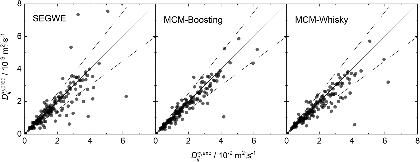 | ||
| Fig. 8 Parity plots of the predictions (pred) of D∞ij with SEGWE and both hybrid MCMs developed in this work over the experimental data (exp) from our reduced database. The solid lines indicate perfect predictions, the dashed lines indicate relative deviations of ±25%. | ||
The parity plots for the two hybrid MCMs show a narrow spread of the data points around perfect predictions (solid lines) and in general only few outliers that are predicted with very large deviation; most of the predicted data points lie within the ±25% boundaries (dashed lines). Slightly more data points are underestimated by MCM-Whisky compared to MCM-Boosting, which is the reason for the slightly higher rMAE and rRMSE scores. In contrast, SEGWE shows a comparatively large number of predictions outside the ±25% boundaries.
The results of MCM-Boosting (the overall best-performing MCM) are also compared to those of SEGWE (the overall best-performing semiempirical model) in a histogram representation in Fig. 9, which shows the number of data points that are predicted with a certain relative deviation from the experimental data.
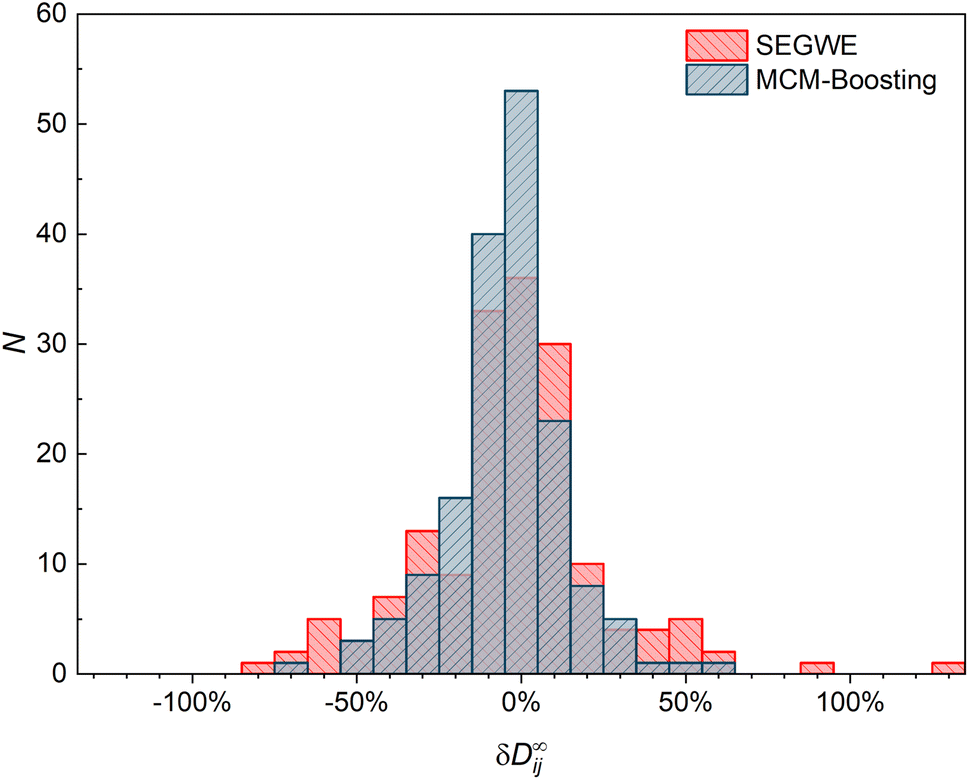 | ||
| Fig. 9 Histogram of the number of data points N from the reduced database that are predicted with a defined relative deviation from the respective experimental data δD∞ij = (D∞,predij − D∞,expij)/D∞,expij by SEGWE (red) and MCM-Boosting (blue). | ||
Fig. 9 underpins the performance of the hybrid MCM-Boosting: more D∞ij are predicted with low deviation compared to the predictions by SEGWE. For instance, 116 data points are predicted with a relative error |δD∞ij| < 15% with MCM-Boosting, whereas for SEGWE, this is the case for only 99 data points. The differences are even clearer when looking at predictions with a relative error |δD∞ij| < 5%: MCM-Boosting predicts 53 mixtures with such high accuracy, versus just 36 in the case of SEGWE.
4.3 Completed database
As a final result, we provide the completed matrices of D∞ij predictions using MCM-Boosting and MCM-Whisky for the 10608 possible combinations of all 208 solutes i and 51 solvents j from the full database, as introduced in Section 2. In this case, the MCMs have not been trained following a leave-one-out strategy, but using all data points from the database; the same hyperparameters were thereby used as in the previously described analysis. The complete predicted data set is provided in a machine-readable format, namely as a .csv file, as part of the ESI,† together with the learned feature vectors ui and vj, from which the data can also be constructed. If predictions for unstudied D∞ij are required, they can be taken from this table.
For MCM-Boosting, the completed matrix of D∞ij predictions is visualized in Fig. 10, together with the uncertainties of the predictions. The corresponding visualization for MCM-Whisky is in Fig. S.4 of the ESI.†
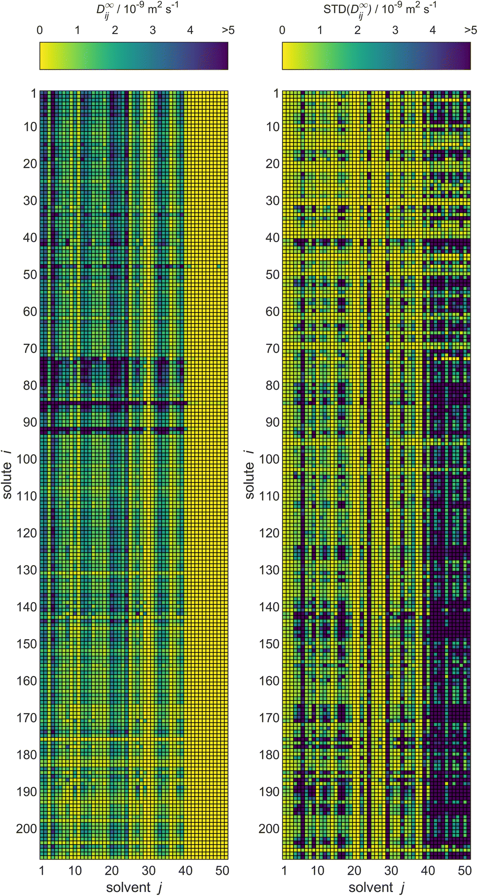 | ||
| Fig. 10 Predictions of D∞ij by MCM-Boosting (left) and the uncertainties of the predictions (right) for all solutes i and solvents j (identified by numbers, see Table S.1 in the ESI†) from the full database. The color code indicates the values of D∞ij. | ||
A significant advantage of the Bayesian approach of matrix completion, which we have followed here, is that probability distributions for all predicted D∞ij with the MCMs are obtained. This allows us to report not only the predictions for D∞ij, but also the corresponding uncertainties. That information is also provided both for MCM-Boosting and MCM-Whisky in the .csv files in the ESI.†
The methods presented in this work were applied here only to a single isotherm. The semiempirical models, on the other hand, describe diffusion data at arbitrary temperatures. In principle, the studies done in this work could be extended to include the influence of the temperature on D∞ij, as it was done by Damay et al. for the prediction of activity coefficients at infinite dilution.28 However, such an endeavour is likely to encounter problems as the database on D∞ij is extremely narrow outside the range of ambient temperatures, cf.Fig. 2. To achieve substantial advances, we need more data, and in particular more data that covers a wider temperature range.
5 Conclusions
In the present work, we provide a comprehensive database of liquid phase diffusion coefficients at infinite dilution D∞ij in binary mixtures at 298.15 ± 1 K. The database contains 353 experimental data points for D∞ij, which were mainly extrapolated from concentration-dependent data, and covers 208 solutes i and 51 solvents j. We have used the new database for systematically evaluating four established semiempirical models for predicting D∞ij, namely the methods of Wilke and Chang, Reddy and Doraiswamy, Tyn and Calus, and SEGWE; the best performance was found for the most recent of these models, which is SEGWE.Furthermore, we have developed novel methods for the prediction of D∞ij based on the machine-learning concept of matrix completion. Three such matrix completion methods (MCMs) are presented here: a purely data-driven MCM, which was trained only on the data on the experimental D∞ij from our database, and two hybrid MCMs that combine information from SEGWE with the experimental data. The purely data-driven MCM suffers from the sparsity of the available data and performs not as well as the semiempirical models. This is different for the two hybrid MCMs, for which significant improvements in terms of predictive accuracy compared to all semiempirical models were found.
As a result, we report values for all 10608 D∞ij for the studied solutes and solvents, which includes a large number of novel data points. We also provide the expected accuracy of the predictions in form of model uncertainties, which is in most cases not much different than typical deviations between experimental values for D∞ij for the same mixture reported by different authors. Such data may also be instrumental in the design of experiments, which is especially relevant considering the sparse availability of experimental data on D∞ij.
The results of the present work, in particular the surprisingly good performance of the hybrid MCMs, motivate an extension to other conditions and the application of MCMs to the prediction of further thermophysical properties in future work. It is interesting to note that the matrix completion approach emerges not as a competitor to the established methods, but rather as a complement. Its full potential is unlocked in the combination with the semiempirical models, which leads to significant improvements in the prediction of diffusion coefficients. We therefore consider this work as an inspiration to future investigations of coupling ML approaches with existing thermophysical models to create the next generation of powerful hybrid predictive models.
Data availability
The data sets supporting this article have been uploaded in tabular form as part of the ESI.† Furthermore, these data sets, together with all predictions for D∞ij from the hybrid MCMs, have been uploaded in a machine readable format (.csv) as part of the ESI.† For some individual data points, restrictions to the availability apply. These data were used under license for this study and are marked as such; they are available directly from Dortmund Data Bank (DDB) version 2019. The complete Stan code used in processing the data sets in this work has also been uploaded as part of the ESI.†Conflicts of interest
There are no conflicts to declare.Acknowledgements
This project has received funding from the European Union's Horizon 2020 research and innovation programme under grant agreement No. 694807. The authors furthermore gratefully acknowledge financial support by Carl Zeiss Foundation in the frame of the project “Process Engineering 4.0” and by Bundesministerium für Wirtschaft und Klimaschutz (BMWK) in the frame of the project “KEEN”, as well as kind support by DDBST GmbH.Notes and references
- A. Vignes, Ind. Eng. Chem. Fundam., 1966, 5, 189–199 CrossRef CAS.
- H. A. Kooijman and R. Taylor, Ind. Eng. Chem. Res., 1991, 30, 1217–1222 CrossRef CAS.
- Dortmund Data Bank, 2019, https://www.ddbst.com.
- F. Jirasek, R. A. S. Alves, J. Damay, R. A. Vandermeulen, R. Bamler, M. Bortz, S. Mandt, M. Kloft and H. Hasse, J. Phys. Chem. Lett., 2020, 11, 981–985 CrossRef CAS PubMed.
- D. Bellaire, O. Großmann, K. Münnemann and H. Hasse, J. Chem. Thermodyn., 2022, 166, 106691 CrossRef CAS.
- R. Taylor and R. Krishna, Multicomponent Mass Transfer, Wiley, New York, 1993 Search PubMed.
- C. R. Wilke and P. Chang, AIChE J., 1955, 1, 264–270 CrossRef CAS.
- K. A. Reddy and L. K. Doraiswamy, Ind. Eng. Chem. Fundam., 1967, 6, 77–79 CrossRef CAS.
- M. T. Tyn and W. F. Calus, J. Chem. Eng. Data, 1975, 20, 106–109 CrossRef CAS.
- R. Evans, G. Dal Poggetto, M. Nilsson and G. A. Morris, Anal. Chem., 2018, 90, 3987–3994 CrossRef CAS PubMed.
- A. Einstein, Ann. Phys., 1905, 322, 549–560 CrossRef.
- B. E. Poling, J. M. Prausnitz and J. P. O'Connell, The Properties of Gases and Liquids, McGraw-Hill, New York, 2001 Search PubMed.
- C. A. Crutchfield and D. J. Harris, J. Magn. Reson., 2007, 185, 179–182 CrossRef CAS PubMed.
- D. Li, I. Keresztes, R. Hopson and P. G. Williard, Acc. Chem. Res., 2009, 42, 270–280 CrossRef CAS PubMed.
- R. Neufeld and D. Stalke, Chem. Sci., 2015, 6, 3354–3364 RSC.
- R. Evans, Prog. Nucl. Magn. Reson. Spectrosc., 2020, 117, 33–69 CrossRef CAS PubMed.
- F. Jirasek and H. Hasse, Fluid Phase Equilib., 2021, 549, 113206 CrossRef CAS.
- R. Ramprasad, R. Batra, G. Pilania, A. Mannodi-Kanakkithodi and C. Kim, npj Comput. Mater., 2017, 3, 1–13 CrossRef.
- K. T. Butler, D. W. Davies, H. Cartwright, O. Isayev and A. Walsh, Nature, 2018, 559, 547–555 CrossRef CAS PubMed.
- V. Venkatasubramanian, AIChE J., 2019, 65, 466–478 CrossRef CAS.
- A. R. Katritzky, M. Kuanar, S. Slavov, C. D. Hall, M. Karelson, I. Kahn and D. A. Dobchev, Chem. Rev., 2010, 110, 5714–5789 CrossRef CAS PubMed.
- A. Abbasi and R. Eslamloueyan, Chemom. Intell. Lab. Syst., 2014, 132, 39–51 CrossRef CAS.
- R. Beigzadeh, M. Rahimi and S. R. Shabanian, Fluid Phase Equilib., 2012, 331, 48–57 CrossRef CAS.
- F. Gharagheizi and M. Sattari, SAR QSAR Environ. Res., 2009, 20, 267–285 CrossRef CAS PubMed.
- A. Khajeh and M. R. Rasaei, Struct. Chem., 2012, 23, 399–406 CrossRef CAS.
- H.-J. Xue, X.-Y. Dai, J. Zhang, S. Huang and J. Chen, Proceedings of the 26th International Joint Conference on Artificial Intelligence, Melbourne, Australia, 2017, pp. 3203–3209 Search PubMed.
- M. J. Pazzani and D. Billsus, The Adaptive Web: Methods and Strategies of Web Personalization, Springer Berlin, Heidelberg, 2007, pp. 325–341 Search PubMed.
- J. Damay, F. Jirasek, M. Kloft, M. Bortz and H. Hasse, Ind. Eng. Chem. Res., 2021, 60, 14564–14578 CrossRef CAS.
- F. Jirasek, R. Bamler and S. Mandt, Chem. Commun., 2020, 56, 12407–12410 RSC.
- F. Jirasek, R. Bamler, S. Fellenz, M. Bortz, M. Kloft, S. Mandt and H. Hasse, Chem. Sci., 2022, 13, 4854–4862 RSC.
- N. Hayer, F. Jirasek and H. Hasse, AIChE J., 2022, 68, e17753 CrossRef CAS.
- S. K. Raghuwanshi and R. K. Pateriya, Data, Engineering and Applications: Volume 1, Springer, Singapore, 2019, pp. 11–21 Search PubMed.
- R. L. Rowley, W. V. Wilding, J. L. Oscarson, Y. Yang, N. A. Zundel, T. E. Daubert and R. P. Danner, DIPPR Data Compilation of Pure Chemical Properties, Design Institute for Physical Properties, AIChE, Database date: 2018, retrieved via The DIPPR Information and Data Evaluation Manager for the Design Institute for Physical Properties – Version 12.3.0 (May 2018 Public), https://www.aiche.org/dippr, 2003 Search PubMed.
- K. P. Murphy, Machine Learning: A Probabilistic Perspective, MIT Press, Cambridge, MA, 2012 Search PubMed.
- C. Zhang, J. Butepage, H. Kjellstrom and S. Mandt, IEEE Trans. Pattern Anal. Mach. Intell., 2019, 41, 2008–2026 Search PubMed.
- D. M. Blei, A. Kucukelbir and J. D. McAuliffe, J. Am. Stat. Assoc., 2017, 112, 859–877 CrossRef CAS.
- A. Kucukelbir, D. Tran, R. Ranganath, A. Gelman and D. M. Blei, J. Mach. Learn. Res., 2017, 18, 1–45 Search PubMed.
- B. Carpenter, A. Gelman, M. D. Hoffman, D. Lee, B. Goodrich, M. Betancourt, M. A. Brubaker, J. Guo, P. Li and A. Riddell, J. Stat. Software, 2017, 76, 1–32 Search PubMed.
- R. E. Schapire, Mach. Learn., 1990, 5, 197–227 Search PubMed.
- G. C. Cawley and N. L. C. Talbot, Pattern Recogn., 2003, 36, 2585–2592 CrossRef.
Footnotes |
| † Electronic supplementary information (ESI) available. See https://doi.org/10.1039/d2dd00073c |
| ‡ These authors contributed equally to this work. |
| This journal is © The Royal Society of Chemistry 2022 |