Data-driven generation of perturbation networks for relative binding free energy calculations

Abstract

Relative binding free energy (RBFE) calculations are increasingly used to support the ligand optimisation problem in early-stage drug discovery. Because RBFE calculations frequently rely on alchemical perturbations between ligands in a congeneric series, practitioners are required to estimate an optimal combination of pairwise perturbations for each series. RBFE networks constitute in a collection of edges chosen such that all ligands (nodes) are included in the network, where each edge represents a pairwise RBFE calculation. As there is a vast number of possible configurations it is not trivial to select an optimal perturbation network. Current approaches rely on human intuition and rule-based expert systems for proposing RBFE perturbation networks. This work presents a data-driven alternative to rule-based approaches by using a graph siamese neural network architecture. A novel dataset, RBFE-Space, is presented as a representative and transferable training domain for RBFE machine learning research. The workflow presented in this work matches state-of-the-art programmatic RBFE network generation performance with several key benefits. The workflow provides full transferability of the network generator because RBFE-Space is open-sourced and ready to be applied to other RBFE software. Additionally, the deep learning model represents the first machine-learned predictor of perturbation reliability in RBFE calculations.

---

1 Introduction

Alchemical Free Energy (AFE) calculations have seen significant increase in popularity in both the academic and commercial domains of pharmaceutical development. These types of calculations leverage an alchemical description of a molecular perturbation for the purpose of estimating free energies of binding of ligands to a drug target.^1–4 Absolute Binding Free Energy (ABFE) calculations are not yet routinely used for protein–ligand systems owing to challenges in converging accurate free energy estimates.^5–8 As a result relative binding free energy (RBFE) calculations remain one of the most popular types of AFE techniques, and have become pivotal in modern computational chemistry approaches that support medicinal chemistry campaigns. Its success is largely owed to recent improvements in processing hardware coupled with advances in empirical force fields which has pushed the technique's potential to predict ligand binding affinities with a mean unsigned error below 1 kcal mol⁻¹, at acceptable computational costs.^9–12 The field of RBFE calculations has seen considerable progress over the last several years with both academic and commercial developers pushing its boundaries even further using a variety of community-curated benchmarking series and guidelines.^12–16

The community's performance across the available RBFE benchmarking sets is variable due to the heterogeneity of RBFE implementations. This variability is primarily explained by limitations in used RBFE software. This results in bottlenecks that can be shared across RBFE software, such as inaccuracies when performing scaffold hopping, net charge adjustments or changes in ligand binding modes,^14,17,18 as well as bottlenecks that are unique to certain implementations due to for instance shortcomings in supported empirical force fields.^10,19,20

In RBFE the free energy of binding for a series of compounds is estimated from a set of pairwise binding free energy differences (ΔΔG), which are transformed into binding free energies relative to a common reference value (ΔG) via for instance a regression scheme. This requires the planning of a perturbation network (or graph) that connects all N compounds in a congeneric series using n edges. To connect all ligands to the network, at least N − 1 edges are required (a minimally connected network), and up to edges may be used (a fully connected network). Previous work has shown that accuracy of binding free energy estimation generally increases when the number of edges increases, but the computing expense of a fully connected network becomes rapidly impractical as the size of the congeneric series increases.²¹

If no error was made in the prediction of pairwise binding free energy differences (ΔΔG), each possible network for a congeneric series would yield the same binding free energy estimates (ΔG). In practice the choice of a network has a significant influence on predictive power, because a given RBFE protocol makes errors of a different magnitude for each edge. These errors arise from different sources that reflect fundamental limitations in the technology, for instance forcefield inaccuracies leading to systematic errors, and statistical errors that are introduced due to finite sampling of configurational integrals. Additionally, the performance of free energy difference estimation between pairs of compounds is influenced by numerous implementation specific details (e.g. softcore parameters, topological coupling methodology, λ schedule). Consequently the choice of a network that maximises accuracy and minimises computing expense for a given RBFE protocol is not trivial (Fig. 1). Such tasks have historically been carried out manually by practitioners relying on expertise in a specific RBFE implementation and intuition to select an efficient network. However, with increased adoption of RBFE and a push for routine applications to large datasets such an approach is increasingly impractical. As a consequence it is common practice to generate star-shaped networks (where all ligands are perturbed to a single reference ligand) for large ligand series (n > 50). Although this style of network generation is attractive because of its simplicity, little research has been done to investigate the impact it has on RBFE accuracy.

Fig. 1 The choice of edges that define a perturbation network is essential for RBFE prediction accuracy. (A) Given two network generators (orange and blue, these can be humans or machines), (B) a number of perturbations is chosen between ligands in a congeneric series to form a connected network. For each chosen edge, an RBFE simulation is performed. Each edge produces errors of different magnitude. (C) Relative binding free energies are transformed using for example a regression scheme to obtain per-ligand ΔG_bind estimations in reference to one of the series' ligands. (D) Compared to experimental binding free energies, different perturbation network topologies have different predictive power. In this example, the blue network outperforms the orange because the latter has multiple outliers.

Lead Optimization Mapper (LOMAP²²) is the primary programmatic approach to RBFE network generation and is used in diverse RBFE software implementations including Flare.^23,24 The LOMAP approach is critically based on LOMAP-Score which is a model metric for the reliability or precision of a given RBFE perturbation, i.e. whether it is possible to get a converged estimate with reasonable computing effort. The LOMAP algorithm in its current form relies on expert knowledge in the form of rules that influence the LOMAP-Score. For example, within the LOMAP-Score algorithm a perturbation between a pair of molecules involving removal of a sulfonamide moiety would be penalised heavily as the errors associated with this perturbation in the context of other molecules has been found to be high during testing of the RBFE software in question. Conversely, a perturbation involving replacement of a hydrogen by a fluorine on an aromatic ring would result in relatively high LOMAP-Score as errors for this class of perturbation have been found to be low during testing. Because the collection of perturbations that would ever be performed in RBFE is sufficiently large to prohibit rule generation for all of them, LOMAP-Score models errors imperfectly, resulting in sub-optimal RBFE network design. Additionally, the set of rules in LOMAP-Score has been fine-tuned for years by RBFE experts in order to make it perform acceptably for specific implementations; this has decreased transferability of LOMAP-Score between diverse RBFE implementations. Examples of these additions to LOMAP-Score rules can be found in the original LOMAP repository commit history.‡

In practice and in an effort to deal with these shortcomings retrospective RBFE benchmarking studies often feature networks that have been adjusted manually using a LOMAP generated network as a starting point. In almost all cases there is an opacity as to how these networks are augmented, and it is likely that additional edges are frequently added iteratively upon examination of the initial RBFE campaign's accuracy versus experimental measures. Although it can be argued that the augmented RBFE network is a better representation of the specific RBFE implementation's predictiveness, this practice decreases comparability between implementation as augmentation is highly dependent on human expertise. Additionally, as not all RBFE practitioners hold expert knowledge for network augmentation, this practice delivers an overstated picture of the true performance of the RBFE implementation in question when applied prospectively. This highlights the need for an objective approach in RBFE network generation that is not based on expert knowledge.

More recently, data-driven approaches based on optimal design that offer a theoretically more objective approach have been proposed.^25,26 Although promising alternatives to LOMAP, these algorithms are still in active development. Notably, NetBFE uses an iterative exploration of congeneric series using knowledge of edge precision gained incrementally by processing specific edges in the RBFE network;²⁶ an initial estimation of edge precision is thus important in this approach. However, a robust edge precision predictor is currently absent in the field of RBFE, forcing some approaches to revert back to simpler metrics such as molecular similarity.²¹ Additionally, novel machine learning (ML) techniques of describing RBFE perturbations have been proposed in the form of siamese neural networks.^27,28

The current work proposes a data-driven RBFE network generator as an alternative to expert-driven approaches. To accomplish this, a transfer learning ML framework was designed that allows predictions of statistical uncertainties for molecular perturbations typically handled in RBFE. Using such predictions for all possible pairs in a given congeneric series, a data-driven RBFE network can be generated. The approach was implemented in LOMAP to generate networks using predicted statistical uncertainties as input metric instead of the default LOMAP-Score.

This work presents several concepts novel to the field of RBFE network generation. RBFE-Space, a transferable training domain that is composed of a large number of RBFE perturbations (n ∼ 4000) was created for this work and has been made publicly available to further drive ML research in the field of RBFE. The predictor leverages a novel siamese neural network architecture using graph neural network (GNN) legs. The ML predictor is shown to predict statistical uncertainties more accurately than the expert-driven LOMAP-Score. Finally, a fully-connected network of the TYK2 RBFE benchmarking series was simulated; network analysis on this dataset has revealed several key learning points for RBFE network generation. The prototype data-driven RBFE network generator already performs comparatively to state-of-the-art network generators, is transferable between RBFE implementations and can be objectively improved by training set expansion.

2 Methods

We start by defining the error made on predicting a pairwise binding free energy difference between a pair of compounds A–B with a given RBFE protocol as:where RBFE and EXP are relative binding free energy prediction and experimental measures, respectively. This heuristic has been previously described by our group and has been used to generate ML models for post-hoc correction of free energy predictions.²⁹

We hypothesize that edges in a RBFE network with low precisions are associated with low |ΔΔG_offset| values. This hypothesis reflects the empirical observation that, for a given protocol, RBFE predictions with large statistical uncertainties rarely give accurate estimates of experimental measures. Of course a highly precise RBFE edge prediction could significantly deviate from the experimental measure due to systematic protocol errors (for instance due to a poor description of the energetics by the chosen forcefield), but as long as a reasonable correlation is observed, networks selected according to this metric will approximate the optimal choice. The chief motivation for this assumption is that it only requires estimation of the statistical uncertainty of edges for a given RBFE protocol, which can be done without knowledge of the experimental measure. Later we will show that this hypothesis is supported by data.

However estimating statistical uncertainties for every given possible edges in a network via for instance calculation of the standard error of the mean binding free energy change (ΔΔG_bind SEM) would be impractically time-consuming. Our task is therefore to find a descriptor that approximates ΔΔG_bind SEM and that can be inexpensively computed to plan an RBFE campaign. To do so we turn to machine learning (ML). Subsections 2.1–2.3 outline the associated methodological steps (training set generation, model training, and model applications).

2.1 Generation of a training set that encompasses RBFE-Space

ML predictors of the precision of an RBFE calculation can in principle be derived using a sufficiently large training set that includes all possible examples of alchemical perturbations between congeneric series. However computing ΔΔG_bind SEM for a training set representative of drug-like chemical space is computationally intractable owing to the size of the training set required. To address this issue we propose the following abstractions: (1) representative RBFE perturbations between compounds in congeneric series reported in the literature are mapped onto a benzene ring (Section 2.1.1; Fig. 2); (2) the SEM of the perturbation is estimated by computing free energy changes in an simplified environment. Various representations were considered (e.g. vacuum) and an aqueous phase environment (Section 2.1.2) was selected to offer a condensed phase description at a computationally affordable cost.

Fig. 2 Example grafting of a molecular perturbation onto a benzene scaffold as applied during creation of RBFE-Space. Shown is an example of a molecular perturbation typical in RBFE between two analogues of omeprazole (left-hand side), where the maximum common substructure (MCS) is shown in black. Grafting R-groups 1 & 2 onto a common benzene scaffold results in a generalised representation of the perturbation (right-hand side). In the RBFE-Space derivative, the chlorine R-group on the first ligand (chlorobenzene) is forced to vanish from the first carbon of the MCS towards the second ligand (benzyl fluoride): in practice this entails changing the chlorine atom into a hydrogen atom. In the same perturbation, the fluoromethyl group is grown on the second carbon atom of the benzene MCS. The anchor symbol denotes the aliphatic carbon atom that is used as a bridge for the methyl/fluorine in R-group 2. See Section 2.1.1 for a detailed description of the methodology.

2.1.1 Grafting of benchmarking series perturbations onto a common benzene scaffold. To build a collection of representative RBFE perturbations, data was drawn from all publicly available FEP benchmarking series (total 18) as defined in recent work from the Open Force Field Initiative and Merck.^13,15 Within each series, all possible pairs of ligands were picked. Next, perturbations that involved ten or more heavy atoms perturbed or a change in formal charge were discarded (as these were deemed likely to be highly unreliable with the chosen RBFE protocol).

Using primarily the python library RDKit³⁰(2020.09.5), R-groups were extracted through manipulation of SMARTS-patterns generated from per-pair maximum common substructure (MCS) analyses. The ‘anchor’ atom for each R-group (i.e. the first atom in the MCS that a given R-group is attached to) was stored. Then, for each member ligand of all perturbations in the dataset, the R-groups were grafted onto benzene molecules while using the anchor atom as a linker, except for cases where the anchor atom was an aromatic carbon atom in which case no anchor atom linker was used (see Fig. 2). The main ideas for the code of this protocol were inspired by blogposts by Landrum and Schmidtke.^31,32 Whereas grafting a simple (e.g. chlorine addition) perturbation is straightforward, more complex perturbations involving for example multiple fused rings or more than six R groups were excluded for simplicity as grafting these becomes exceedingly complex and does not add significant knowledge to the training domain. Additionally, perturbations that involved a benzene ring without other constituents were excluded as these would cause issues when generating an MCS for the RBFE protocol, since this code largely depended on enforcing the benzene scaffold based on its topology. After removing duplicates and the grafting step the complete RBFE-Space dataset consisted of 3964 perturbations saved as dual SMILES entries.

2.1.2 Molecular dynamics simulations and free energy calculations. For each pair, a RBFE protocol was set up using BioSimSpace³³ (v2020.1.0 py37h9bf148f_593). For each benzene derivative pair in RBFE-Space, SMILES for ligand 1 and ligand 2 were parsed and an MCS was found while allowing ring breaking and ring size changing. After aligning ligands 1 and 2, a single, perturbable merged ligand was created from the two input molecules that contained the properties of both input ligands. The used atom mapping (that describes which R-groups were being perturbed into which between ligands) was stored. This ‘merged ligand’ was then solvated in a 3 nm³ cubic box with TIP3P waters. Simulations were set up with the engine SOMD^23,34,35 using 10 000 moves, 50 cycles and a 2 fs timestep, adding up to 1 ns simulation time per λ window. Each perturbation was set to consist in 11 equidistant λ windows (i.e. λ ∈ [0.0, 0.1, … 1.0]). Each perturbation was run in quintuplicate.

Simulations for this work were run using on a variety of computing clusters (Ubuntu 16.01) mostly containing Nvidia GeForce GTX 1080 and 980 GPU cards. The walltime per window for the above described protocol was 8–12 minutes, depending on system size and hardware, totalling to ∼24 000 GPUh for the complete series of runs.

For each perturbation the free energy change ΔG_solvated was estimated using pymbar³⁶ with subsampling enabled, and discarding the first 5% of the trajectories. The SEM of a given perturbation was computed as the standard error of the mean across each quintuplicate in RBFE-Space:

where n = 5 and σ is the standard deviation across the samples of ΔG_solvated in each quintuplicate, calculated aswhere is the mean of the five predicted relative free energies of solvation for the given perturbation. For all perturbations in RBFE-Space that were simulated in both directions (i.e. both A → B and B → A), SEM values were balanced by reporting the mean SEM value for both perturbations.

The TYK2 and TNKS2 series' RBFE perturbations were run on the same hardware as RBFE-Space simulations. Prior to system setup, proteins were prepared using Flare V4. Ligands (GAFF2) and proteins (FF99SB) were parameterised using BioSimSpace (which uses LEaP, Antechamber and Parmchk) and solvated in TIP3P waterboxes (10 Å orthorhombic shell). Each system (i.e. the ligand, protein and waters) was energy minimised (250 steps) and pre-equilibrated at λ = 0.0 using a sequence of NVT and NPT equilibration with cuda.pmemd using the BioSimSpace API. As with RBFE-Space simulations, 11 λ windows were used for each ligand perturbation, but with 4 ns of sampling instead of 1 ns (initial tests showed that 1 ns of sampling was insufficient for systems of this complexity). For each perturbation, relative free energies of solvation and binding in kcal mol⁻¹ were estimated using pymbar with subsampling enabled, and discarding the first 5% of each trajectory to allow for re-equilibration at each λ value.

2.2 Training of machine-learning models that predict RBFE statistical errors

Given the complete RBFE-Space training domain with calculated values as per eqn (2), ML models were trained to predict this value for a newly-presented perturbation. From here on, values predicted by ML models will be referred to as .

All ML code was executed using the Keras implementation of TensorFlow 2.6.0. All models (pre-training, transfer-learning and fine-tuning) were run using a LogCosh loss function and Adam optimiser with an initial learning rate of 5 × 10⁻⁷. All ML models were run on a system running Ubuntu 18.04.4 LTS with 20 CPU cores (Intel(R) Core(TM) i9-7900X CPU @ 3.30 GHz) and four Nvidia GeForce GTX 1080 GPU cards using CUDA 11.2.

2.2.1 Main RBFENN model architecture based on siamese neural networks. To model perturbations between two molecules a novel approach based on siamese neural networks^37,38 was adopted (Fig. 3). This approach has been used in other work for image recognition in low-data regimes where the goal has been to distinguish between images in the testing domain. Typically this approach consists of three concepts: (1) a two-legged structure, where each ‘leg’ has one input, (2) shared weights between legs such that the legs learn the same encoding and (3) some form of similarity (e.g. Euclidian distance) layer that computes the degree to which encodings overlap.

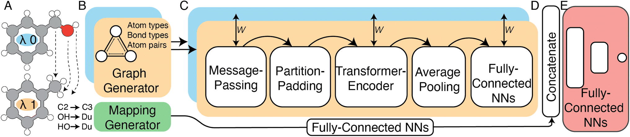Fig. 3 High-level schematic representation of the siamese Relative Binding Free Energy Neural Network (RBFENN) architecture. (A) Two ligand structures are input as SMILES, where each ligand represents either λ endstate of a given RBFE perturbation. (B) Molecular structures are described as graphs using atom types, bond types and bonds as descriptors. (C) The bi-legged graph neural network (GNN) component of the architecture that consists of a message-passing neural network sequence ending in several feed forward NN layers. Training weights are shared between the two legs (orange and blue) of this component. (D) A concatenation layer merges the signal of the two input legs (orange and blue) as well as the atom mapping between λ endstates which has been passed through several feed forward NNS. E: multiple feed forward NN layers with linearly decreasing numbers of neurons resulting in a single neuron with a linear activation function. Note that the all layers in Section C are frozen during the pre-training stage of the transfer-learning phase described in Section 2.2.2. See Fig. S1† for lower-level details on the model architecture.

In this work a modified siamese neural network (‘RBFENN’) was used that adopts concept (1) and (2), but does not let a similarity layer compute distance. The rationale behind using shared weights is that for a given ligand perturbation, either direction (e.g. growing or vanishing an R-group) entails roughly the same SEM in RBFE. Because the intended prediction label in this work is , not similarity, a concatenation layer was used to join legs of the neural network. After the concatenation layer, several fully-connected layers were used with decreasing numbers of neurons leading to the final single neuron. All fully-connected layers used in the network used ReLu activation function, whereas the final single neuron used a linear activation function. See Fig. S1† for a low-level overview of the RBFENN architecture.

To encode the chemistry of input structures (ligands A and B) a per-leg message-passing neural network (MPNN) was used. Input graphs were populated with three inputs, namely atom features (element, #valence electrons, #hydrogen bonds, orbital hybridisation), bond features (bond type, conjugation) and atom pair indices. Whereas the MPNN architecture was based on previous work by Gilmer³⁹ and DeepChem,⁴⁰ the code implementation of this work was primarily based on examples provided by Kensert.⁴¹ Based on information provided during RBFE setup, the atom-mapping (i.e. which R-groups are transformed to which between ligands A and B) is expressed as an array of 50 integers, where each integer index relates to the atom index in ligand A, and the integer value relates to the atom index in ligand B. To effectively learn atom-mappings between two input molecules, the model must be able to relate atom-mapping information to the input graphs; atom-mappings are presented to the model using atom indices. It is assumed that the model learns atom indexing which is reasonable because the algorithm for graph generation in the MPNN algorithm uses atom indexing to represent bonds in each ligand encoding. Because no training ligands' mappings contained more than 50 atoms, all non-matched values in the mapping array were set to 99 to represent a non-match.

Although the number of allowed epochs was set to 5000, an early-stopping callback was set to quit training when models started overfitting by monitoring mean absolute validation error; the callback was set to restore the model with the lowest validation error.

2.2.2 Transfer-learning approach. To deal with the low-data regime (n = 3964, see Section 2.1.1) and the added model complexity of an MPNN (see Section 2.2.1), a transfer-learning⁴² approach was adopted that uses a pre-training regime to learn molecular encodings on a larger dataset with a cheaply computed label. In this way, the RBFENN can be pre-trained on a domain of n = 2550² − 2550 ≈ 6.5 × 10⁶ points (i.e. composed of all possible pairs of molecules in RBFE-Space); as a cheaply computed label the difference in estimated solubility^43,44 (ΔESOL) was used. This property was chosen not because it is necessarily meaningful to this work's purposes, but because it is a complex descriptor that pushes the RBFENN to learn a more complete understanding of chemical structure a priori; similar approaches have been reported.^45,46 Early-stopping patience for this phase was set to 5 epochs as early convergence (70–100 epochs) was observed. For the pre-training phase, 800 000 training samples and 200 000 validation samples were used to save memory and because it was observed that larger training/validation sets did not sufficiently improve model training.

Subsequent to pre-training, model weights from the pre-training phase were loaded and the last four fully-connected layers were replaced with re-initialised (i.e. weights set to 0) layers. All other pre-trained layers of the RBFENN (MPNN legs and concatenation layer) were ‘frozen’ by setting layer trainable = False for each layer. In this transfer-learning phase, the RBFENN that has learned to encode chemical structure input learns to predict (instead of ΔESOL) by training the newly initialised fully-connected layers on the 2550 SEM samples in RBFE-Space. For this phase, a k-fold cross-validation approach was used where k = 5.

For each k-fold model in the transfer-learning phase, fine-tuning was performed by unfreezing all layers (i.e. layer trainable = True) and training all layers in an attempt to further minimise validation loss. Both the transfer-learning and fine-tuning phases used a maximum of 5000 epochs with early stopping patience set to 101 epochs. Training was repeated for 9 replicates. Model predictions discussed from here on are thus mean predictions across 5 × 9 = 45 models.

2.2.3 Baseline shallow machine learning model training. A selection of non-neural-network ML models were used to benchmark the RBFENN model performance against. Similar to previous work,²⁹ three different descriptors were used:

• APFP: Atom pair fingerprints as computed using RDKit with a hash length of 256 bits.

• ECFP: Extended connectivity fingerprints as computed using RDKit with a diameter of 6 Å and 1024 bits.

• Molecular properties as computed using Mordred⁴⁷ with all 2D descriptors enabled (n = 1613) where empty fields were replaced with zeroes.

Because featurisation in this case deals with molecular perturbation and not single molecules, a fingerprint subtraction technique was used where each bit value of ligand B is subtracted from the bit value of ligand A.⁴⁸ For each descriptor type, the featurized RBFE-Space was normalised and dimensionalities were reduced using principal component analysis (PCA) using the SKLearn implementation set to keep the 100 most contributing components.

Two shallow ML algorithms were trained using each of the three descriptor training sets of RBFE-Space:

• RF: Random forest regressor using default hyperparameters.

• SVR: Support vector machine regressor using default hyperparameters, with the exception of γ which was set to 1 × 10⁻⁸.

Normalisation data, fit PCA objects and fit ML models were pickled for testing phases.

2.3 Application of RBFE SEM predictions to network generation problems

As outlined in Section 2.2.2, an ensemble of 9 -predicting RBFENNs was generated. From here on, a given prediction for a perturbation between two ligands is computed as the mean of the ensemble's predictions, but is still denoted as .

2.3.1 Featurising test sets for network prediction. For a given congeneric series' collection of ligand files, a fully-connected network (i.e. all possible pairs of ligands, mono-directional) is generated. For each input perturbation, the RBFE-Space derivatives are created as described in Section 2.1. To ensure that the correct perturbation is represented in the atom-mapping array, all atoms of the input ligands that change AMBER atom-type in the perturbation are stored. Then, by forcing the MCS on the six aromatic carbons of the benzene scaffold of the RBFE-Space derivatives, and generating the AMBER atom-type changes with that mapping, the atom-type change information is compared to the input ligands' atom-type information. By rotating the benzene scaffold forced MCS on one of the ligands (e.g. where {0 : 0, 1 : 1, 2 : 2, 3 : 3, 4 : 4, 5 : 5} is the initial forced MCS mapping, a first rotation would be {0 : 1, 1 : 2, 2 : 3, 3 : 4, 4 : 5, 5 : 0}) a second collection of RBFE-Space derivative atom-type changes is created. By repeating this process until all five rotations are completed and picking the mapping that matches the input ligands' mapping atom-type changes, the picked featurised atom-mapping array is ensured to correctly map the per-atom changes between the two ligands.

2.3.2 Processing of predicted SEMs using LOMAP for network generation. A forked version of LOMAP as developed by Cresset for Flare²³ V4 was cloned and implemented into BioSimSpace. As this version of LOMAP allows the usage of user-input scores per ligand pair, values (or other values such as or random values etc…) could be used instead of LOMAP-Score for generating RBFE networks.

Because LOMAP is designed to build networks using the continuous LOMAP-Score that range [0–1] (where 0 is a supposed unreliable edge and 1 is a supposed reliable edge), user-input values needed to be transformed to fit this range. For an example array of SEM values [SEM] that contains all possible combinations of ligands in a congeneric series, the array was scaled to the range [0–1] such that

where [SEM]_inv is computed as

Eqn (4) and (5) applied to , and |ΔΔG_offset| result in , and |ΔΔG^scaled_offset|, respectively. These arrays offer the ability to be ported into the LOMAP network generating algorithm as they match the range and direction of LOMAP-Score. SEM values were inversed such that perturbations with large SEM have a low score. For the sake of simplicity a simple inversion was used in this work but other transformations could be explored in future work. To avoid cumbersome notation, the scaled upperscript symbol is excluded from here on unless otherwise specified.

2.3.3 Network generation and analysis. BioSimSpace³³ (v2020.1.0 py37h9bf148f_593) was used to generate RBFE networks. The main software that handle network generation internally are LOMAP (edge selection; as implemented in Flare V4), RDKit 2020.09.3 (molecular manipulation), networkx 2.6.3 (network manipulation) and matplotlib 3.4.3 with pydot 1.4.2 (network plotting). Similarities between networks (for the same congeneric series) were computed as the percentage of edge overlap between the two networks: given the number of overlapping edges, the percentage relative to both network sizes (n-edges) was computed. The mean percentage was taken as the final network overlap percentage.

Given a set of RBFE predictions, the statistical performance versus experimental ligand binding affinities can be estimated. Whereas a per-edge (‘pairwise’) statistical analysis is meaningful, in this work a per-ligand free energy estimation is made using a weighted least squares method implemented in FreeEnergyWorkflows.⁴⁹ This implementation is equivalent to eqn (2)–(4) of Yang et al.⁵⁰ with weights set as the reciprocal of the propagated standard error of the mean values across the replicates of each RBFE leg (solvated and bound) in kcal mol⁻¹. Pearson R, Mean Unsigned Error (MUE) and Kendall τ metrics were estimated using a bootstrapping approach set to 10 000 repeats. Further plotting methodologies adhered to best practices.¹⁴

3 Results and discussion

3.1 Creation of a training domain that encompasses RBFE-space

3.1.1 RBFE-space characteristics. Molecular simulations were performed for perturbations grafted onto a common benzene scaffold (Fig. 2 and Section 2.1.1) to serve as a training set that captures the space of perturbations that are performed in typical RBFE campaigns. To generate this set, available RBFE benchmarking series were selected and all perturbations within each were extracted and grafted onto benzene (Fig. 4E). Duplicate perturbations and perturbations that involved ten or more perturbed heavy atoms were discarded which resulted in a training set of 3964 points (starting from 16 048). Across this set, the number of perturbed heavy atoms was uniformly distributed (frequency of 400–500 points for 1–9 heavy atoms), except for isomeric perturbations (i.e. a swap in position of two heavy atoms) of which only 46 were simulated (Fig. 4B).

Fig. 4 Summary of RBFE-Space generated using 3964 molecular perturbations grafted onto a common benzene scaffold (Fig. 2). (A) Histogram of values (Section 2.3.2). (B) Histogram of the number of perturbed heavy atoms involved in each perturbation. (C) Scatterplot showing the relation between the change in molecular weight per perturbation in Da and the for each perturbation; colouring shows density (increasing as blue → green → yellow). (D) Boxplots of per perturbation binned by the number of heavy atoms perturbed; horizontal lines in boxes show median values and black diamonds show outliers (95 CI). (E) Histogram that describes how many perturbations of the original congeneric series' were used as templates for grafting onto benzene in RBFE-Space.

values for all perturbations in RBFE-Space showed a distribution that skewed right; the vast majority of values were under 1 kcal mol⁻¹, with a peak frequency of ∼0.15 kcal mol⁻¹ (Fig. 4A). Although no relation is observed between the change in molecular weight and the associated for a given perturbation (Fig. 4C), an increase in median can be observed by increasing the number of heavy atoms perturbed, although it is clear that there are exceptions to this rule as outliers are present in every scale (Fig. 4D). Only direct isomeric perturbations (i.e. n = 0) result exclusively in perturbations with < 0.5 kcal mol⁻¹. Although this relation with the number of perturbed heavy atoms reflects favourably on state-of-the-art MCSS rule-based methods, the noisy nature of this relation suggests that there is scope for more accurate methods to model SEMs of RBFEs. Separating perturbations in this analysis by whether they involve addition (‘Grow’) or removal (‘Shrink’) of heavy atoms does not suggest discernible distributions (Fig. S2†).

3.1.2 The precision of the free energy estimates of RBFE-Space derivatives correlates with the precision of the free energy estimates of their parent ligands. To investigate whether RBFE-Space derivatives are sufficient placeholders to model SEMs of their original ligand counterparts RBFEs, 214 ‘original’ perturbations (i.e. the perturbations from nine publicly available congeneric series) were simulated in quintuplicate for 1 ns per λ window (total 11 windows). Subsequently, all combinations of phases were compared (Fig. 5).

Fig. 5 Correlation scatter plots of SEM values of 214 quintuplicate perturbations in different phases as extracted from publicly available RBFE benchmarking sets (n = 9). The data are shown on a logarithmic scale and points are coloured by the number of heavy atoms that are perturbed in the perturbation (see colour range). Each panel has the data's Pearson R and Kendall τ annotated in its bottom right corner. (A) Solvated versus bound SEMs of ligands with their original scaffold. (B) RBFE-Space derivative (solvated) versus the original scaffold's perturbation in solvated phase. (C) RBFE-Space derivative (solvated) versus the original scaffold's perturbation in bound phase. (D) RBFE-Space derivative (solvated) versus the original scaffold's perturbation ΔΔG_bind value (obtained by ΔG_solvated − ΔG_bound).

For perturbations that give large SEM values quintuplicates runs are insufficient to obtain consistent results for a given edge processed in two directions (A → B or B → A), which introduces noise in correlations of these quantities (Fig. S3,† left-hand side). To remedy this, a logarithmic scale was adopted (Fig. S3,† right-hand side) when comparing SEM (or any other type of variance) arrays, which squashes larger deviations with respect to smaller deviations. This is justified because our approach does not need to estimate accurately large SEM values since edges with large SEM values will be discarded during network generation.

In the following analysis, benzene-grafted perturbations will be referred to as RBFE-Space perturbations, whereas the template perturbation (i.e. with the original ligand scaffolds) will be referred to as original perturbations.

Original solvated SEM values correlate well (R = 0.86) with their bound counterparts, but tend to show lower magnitude (Fig.5A). This is surprising as a bound system has higher complexity than a solvated box – it is expected however that the short sampling time for this analysis (1 ns/λ) was insufficient to relax the protein topology in the simulation, thus enforcing a relatively rigid environment for the ligand perturbation, meaning only a narrow range of conformations could be sampled. Achieving robust estimates of the precision of free energy changes in a bound system is challenging owing to the potential for protein relaxation modes to occur on a broad range of timescales. These observations may also explain why the RBFE-Space SEMs correlate more strongly with bound SEMs than with solvated SEMs. This was deemed acceptable for the present study as we are mainly interested in correlating SEM values.

RBFE-Space SEM values also correlate well to both original solvated, bound SEM values (R = 0.74 and 0.87, resp.) and to ΔΔG_bind SEM values (R = 0.75); a trend in the number of heavy atoms perturbed increasing with higher SEM values can be observed which reflects the trend seen in Fig. 4D.

It should be noted that in this prototypical version of RBFE-Space there is a possibility that R-groups that are separated from each other in the context of an original scaffold will interact with each other when grafted onto a benzene scaffold. Conversely scaffold specific intramolecular interactions with a R-group are lost in the grafting process. We have observed a trend for greater deviation between RBFE-Space and ligand SEM values for cases where bulky R-groups are being simultaneously grown and vanished in the same perturbation. Although not investigated in depth, this issue is assumed to be present in a small population of RBFE-Space, and will have to be resolved in future versions of the dataset. Early solutions to this problem could for instance place the second R-group on the para aromatic carbon of the benzene scaffold; however any third (or more) R-groups will reintroduce the issue. Alternatively, larger scaffolds could be explored.

The main objective of this analysis is to assess whether the RBFE-Space placeholders' SEM values sufficiently correlate to ΔΔG_bind SEM values of their original ligand counterparts (Fig. 5D). Although only moderate correlation has been reached, we postulate that this is a logical effect of simplifying ligand perturbations by grafting them onto a common benzene scaffold. Such simplification was made here to obtain a training domain that is transferable to a variety of congeneric series. Through this simplification, several sources of information are discarded: (1) removal of protein topology and ligand–protein interactions (2) removal of ligand scaffold (interacting with protein or solvent) (3) reduced sampling time (1 ns/λ instead of 4 ns/λ). Whereas all of these could be included in RBFE-Space they would require a significant increase in the size of the training domain to enable development of transferable models.

3.2 Machine-learning models can train on RBFE-space to predict SEMs

To train a machine-learning model on RBFE-Space, a graph neural network (GNN) approach was taken to describe molecular perturbations. This type of architecture was chosen because of its proven potential to learn molecular structures given enough data.^51–53 One major advantage of learning directly the molecular topology instead of pre-computed molecular descriptors is that no prior knowledge of influential descriptors is required. However, when training complex models with many parameters (such as GNNs) care must be taken to provide a sufficiently large training domain to make sure that weights have been optimised to a point where an understanding of chemical structure (or chemical perturbation, in this work's case) has been reached.^51,54 As RBFE-Space contains only 3964 points, we have opted for a pre-training and transfer-learning approach (Fig. 6) which is a technique that has recently gained popularity in chemistry.^46,55,56 In the pre-training phase, a cheaply-computed label, the relative estimated solubility (ΔESOL⁴⁴) was computed for 1 M randomly picked combinations of molecules in RBFE-Space and this training domain was used for pre-training the RBFENN model to learn molecular perturbations. Whereas any chemical descriptor could be picked for this application, ΔESOL is a suitable candidate because it is a relatively complex descriptor which prevents the RBFENN from focussing its learning on a specific chemical detail which would likely happen when learning on simpler properties such as molecular weight or lipophilicity. The pre-training protocol in this approach showed sufficient learning convergence after 100 epochs of training, at which point training was interrupted; the runtime for this step was approximately 9 h.

Fig. 6 Learning curves of the three phases of the RBFENN training protocol for predicting SEM values of RBFE perturbations. (A) Pre-training phase, where a cheaply-computed continuous label (the relative estimated solubility, ΔESOL⁴⁴) was used to generate a training set of 1 M data points using RBFE-Space ligands. Shown are the validation error and training mean absolute errors (MAE; blue and orange, resp.) per epoch. (B) Transfer-learning phase, where the message-passing component (Fig. 3C) weights were forced static (‘frozen’), allowing the remaining layers of the RBFENN to learn to predict SEM rather than ΔESOL while the chemistry-processing layers' weights are retained. Shown in colours are validation MAEs of predicted SEM in kcal mol⁻¹ for five replicates. Shown in gray are training MAEs; all error values are reported as their global minimum value. (C) Fine-tuning phase, where the message-passing component of the RBFENN architecture is allowed to train (i.e. weights are ‘un-frozen’) in an effort to further increase SEM predictivity (panel formatting same as for panel B).

After pre-training, the ΔESOL training domain was discarded and the GNN layers' weights of the RBFENN (Fig. 3C) were ‘frozen’, i.e. their weights were not allowed to be adjusted during training. This transfer-learning phase thus started with a RBFENN architecture that had already learned molecular perturbations. RBFE-Space was then used as a training domain to train the non-frozen layers in the model to predict . Whereas validation MAE varied across replicates, models were observed to converge to 0.4–0.5 kcal mol⁻¹ MAE. In this step, global minimum training MAE values are shown to be higher than global minimum validation MAE values (Fig. 6B). This is likely because of the reduced number of trainable parameters (only weights in 3E are trained) in combination with the low-data regime, where the validation set (20% of RBFE-Space) results in occasional small dynamic ranges, skewing statistics on this subset.

To further maximise the RBFENN predictivity, a fine-tuning phase was performed where all weights of the RBFENN were ‘un-frozen’, i.e. all weights were allowed to be adjusted during training. The idea behind this approach is that the GNN component of the RBFENN can further optimise its predictivity in unison with the remaining layers of the model. Learning curves for this phase show further training of the model, lowering the ensemble MAE to 0.1–0.2 kcal mol⁻¹. Because of the high number of parameters (1 827 712) in this phase rapid overfitting of the training set was observed (training MAE rapidly lowering while validation MAE started increasing). For each replicate, the best-performing (i.e. lowest validation MAE) model at epoch n was extracted and used as the final model. In cases were fine-tuning showed no decrease in validation MAE over the best model in the transfer-learning phase, the top-performing model of the transfer-learning phase was used. Although the validation MAE of the RBFENN ensemble after fine-tuning is ∼0.3 kcal mol⁻¹ and the majority of SEMs in RBFE-Space have values ∼0.15 kcal mol⁻¹ (Fig. 4A), this level of accuracy was considered sufficient to predict perturbations that would exhibit large SEMs (>1.0 kcal mol⁻¹) values.

3.3 Applications of the trained RBFENN

In this section, the RBFENN will be applied to two RBFE benchmarking congeneric series: TYK2 and TNKS2. Although these test sets are present in the training set (Fig. 4), this is assumed acceptable for this work as the majority of perturbations in RBFE-Space have duplicates in other congeneric series. In other words, excluding or including TYK2/TNKS2 in the training set results in essentially the same training set due to the high amount of overlap in R-group modifications present across multiple othercongeneric series. For workflow simplicity these sets were thus included in the training set.

3.3.1 Increasing λ windows in RBFE decreases SEMs. Prior to network generation, λ allocations were benchmarked in the context of RBFE SEM (Fig. S4†) in the solvated phase for six highly reliable and six highly unreliable perturbations in RBFE-Space. The precision (here expressed as of 5 replicates) was recorded at increasing numbers of equidistant λ windows used for MBAR analysis: 3, 5, 9, 17 and 33. For both types of perturbations an exponential decay in was observed; typically convergence was reached at 15–20 λ windows, suggesting further sampling is likely not necessary in RBFE calculations with SOMD for the solvated phase, even for highly unreliable perturbations.

The main objective of this analysis was to determine whether the 11 λ windows protocol used in the generation of RBFE-Space was sufficient to describe SEMs of RBFE perturbations. Although at 11 λ windows convergence does not seem to have been reached in all cases, this number does offer a reasonable approximation of the SEM with acceptable sampling cost. Notably, RBFENN predictions consistently show the correct order of magnitude for all 12 perturbations described in this analysis. This confirms that the estimator can be used to discriminate low precision perturbations from high precision perturbations.

3.3.2 RBFENN-based RBFE networks are distinct from state-of-the-art RBFE networks. RBFE networks generated by LOMAP using LOMAP-Score or RBFENN as edge similarity metrics were compared for the entire public RBFE benchmark set (Table 1). RBFE networks for the TYK2 series show the highest degree of overlap (55%) between the two methodologies. Across the dataset overlaps range from 11% to 47% with an average value of 32%. Some overlap between the methodologies is expected since both input metrics succeed at modelling SEMs to some degree which results in similar assumptions in generating either network. One series of note is Thrombin (11 ligands) which shows 0% overlap. As the compounds in this series are structurally highly similar it is plausible that a large fraction of possible networks minimise equally well precisions. However due to the low number of compounds in the series it is difficult to make statistically-sound comparisons of networks performance.¹³

Table 1 Comparison of RBFENN and LOMAP-Score RBFE networks for all publicly available RBFE benchmarking series in terms of network size (n edges) and overlap (%)^a

Target	Series size (N)	LOMAP-Score network (n)	Network overlap (%)	RBFENN network (n)
a Rows were sorted by ligand series size (N ligands) in descending order. The network overlap was computed by counting the number of overlapping edges between the two networks and computing the mean percentage with respect to the two networks and rounding to the nearest number. EG5 was excluded from this comparison as benzene grafting failed for the majority of the network due to overly complex perturbations. (a–c) These ligand series are further analysed in Sections 3.3.5, 3.3.4 and 3.3.2, respectively.
SYK	44	63	25	64
MCL1	42	61	11	59
HIF2a	42	59	26	64
PFKFB3	40	57	35	60
BACE	36	52	26	51
P38 (MAPK14)	34	45	23	47
CDK8	33	50	44	45
TNKS2^a	21	27	23	24
SHP2	26	38	42	38
PTP1B	23	32	39	33
PDE2	21	29	35	27
Jnk1	21	27	33	27
CDK2	16	21	47	21
TYK2^b	16	23	55	27
c-MET	12	15	37	17
Thrombin	11	13	0	14
Galectin^c	8	10	40	10

---

Because of LOMAP's cluster minimisation and connection algorithm there is typically some variance (±3–4 edges) in the number of edges selected for a congeneric series of N_ligands. We observe in general a relationship of n_edges ≈ 1.4 × N_ligands. Although the number of edges suggested consistently differed between LOMAP-Score and RBFENN networks, no methodology gave a consistently larger network. In general the network overlap percentage between the two methodologies decreases with congeneric series size (thrombin aside). This likely reflects the combinatorial explosion in the number of distinct networks that can be proposed as N_ligands increases.

A visual example of the networks proposed with RBFENN or LOMAP-Score for Galectin RBFE benchmarking series is presented in Fig. 7. Both methodologies make reasonable suggestions, although there is only 40% network overlap between the two network topologies. As visual comparison is a qualitative measurement of RBFE network generation performance and because one of the main objectives of the data-driven approach is to remove the subjective component in the field, a more quantitative approach is pursued in this work.

Fig. 7 Example RBFE networks on the Galectin RBFE benchmarking congeneric series (N = 8). Shown are the state-of-the-art LOMAP-Score approach (orange edges; 10 edges) and novel data-driven approach presented in this work (blue edges; 10 edges). Edges that are present in both RBFE networks are represented as singular black dashed lines. Ligand scaffolds were replaced with black circles for simplification purposes. The ligand scaffold is shown in the center box with the R-group location on the right-hand side of the structure.

3.3.3 RBFENN predicts inexpensively the accuracy of RBFE calculations on TYK2. As the performance of RBFE calculations is determined by the errors made along each edge of the chosen network, different network topologies should result in a difference in the estimation of binding free energies (ΔG) in the limit of finite sampling. A quantitative approach for comparing RBFE networks is thus possible by processing each edge of the networks with the same RBFE protocol, and comparing the estimated binding free energies with experimental data.

To carry out this assessment, the non-receptor tyrosine kinase TYK2 congeneric series¹² was chosen as it is a challenging RBFE benchmarking set of sufficient size to allow reliable statistical analysis.¹³ The TYK2 series also involves a mixture of straightforward ligand sub-groups and more challenging perturbations that involve ring-changes.²³ Additionally, the TYK2 series has been used recently in several RBFE works investigating network generation and machine learning potentials.^26,57 For this series (16 ligands), RBFE was run for all possible perturbations in a single direction ( edges). Monodirectional edges were chosen with the purpose of halving computational cost. The signs of the relative binding free energy predictions for the 120 edges in this RBFE run were inverted to obtain the remaining 120 RBFE predictions, resulting in a bidirectional fully connected network with 240 edges. The validity of this assumption was supported by data generated during creation of the RBFE-Space training set (Fig. S3†).

As stated previously, an ideal RBFE network generator will contain edges with low deviation from experimental measures. Thus edge scoring metrics that correlate more strongly with |ΔΔG_offset| values should select more accurate networks. To verify this, the statistical performances of available heuristics were compared to the |ΔΔG_offset| values (eqn (1)) gathered from the fully connected TYK2 network. The data in Fig. 8A shows that ΔΔG_bind SEM correlates with |ΔΔG_offset|, therefore supporting the hypothesis that selecting edges with lower statistical uncertainties will lead to RBFE networks with lower errors. A possible explanation is that perturbations with greater ΔΔG_bind SEM values involve changes of a greater number of interactions, which would be expected to increase systematic model errors.⁵⁸ In support of this interpretation the data in Fig. 8A shows a trend with the number of heavy atoms perturbed. Fig. 8B shows that this correlation is maintained (albeit more weakly) with RBFE-Space values.

Fig. 8 Scatter plots of |ΔΔG_offset| vs. (A) ΔΔG_bind SEM values for all possible edges in the TYK2 RBFE benchmarking series (120 edges), (B) RBFE-Space SEM values for perturbations included in RBFE-Space (124 edges). The colourbar shows the increase in the number of heavy atoms perturbed per perturbation in the scatter plots. See Table 2 for statistical analyses corresponding to these array comparisons and see Fig. S5† for an extended version of this figure. (C) Scaffold (centre) and analogs in the TYK2 RBFE benchmarking series annotated with ligand names used throughout this work.

Table 2 summarises how different predictors correlate with offset values. As expected ΔΔG_bind shows the strongest correlation, but this metric is computationally too intensive to be of practical use for network generation. Surprisingly edge scoring based on ECFP6 similarity shows no relationship with offset deviations. This is likely because the fingerprint is relatively insensitive to the different perturbations, with most edges assigned a similarity score of around 0.7. The inexpensive estimators RBFENN and LOMAP-Score show comparable correlation with offset deviations. We note there could be many other reasonable proxy variables to the actual |ΔΔG_offset|, and future investigations may well identify descriptors with improved correlations.

Table 2 Statistical performances of various heuristics versus the |ΔΔG_offset| for all possible edges in the TYK2 RBFE benchmarking series (120 edges)

	Pearson R	Kendall τ
a Only perturbations included in RBFE-Space were included (124 edges; see Section 2.1.1). See Fig. S5 for scatterplots corresponding to these array comparisons, and Fig. S6 for distributions of these heuristics.
	0.63	0.46
RBFE-Space SEM^a	0.37	0.28
RBFENN	0.41	0.25
LOMAP-Score	0.42	0.33
ECFP6 similarity	−0.03	−0.01

---

3.3.4 RBFENN matches state-of-the-art for TYK2 RBFE network generation. To the best of our knowledge, this work describes the first fully-connected (FC) RBFE network for the TYK2 series. This dataset allows enumeration of all possible RBFE networks: given a network generator and an edge scoring heuristic the network edge accuracy with respect to experimental data can be determined by looking up edge results in the pre-computed FC network. The number of possible networks is vast. For this dataset there are 16¹⁴ = 7.2 × 10¹⁷ minimally-connected networks (i.e. 15 edges with all nodes included in the network).⁵⁹ The actual number of networks theoretically considered by LOMAP is much greater because of additional heuristics to introduce extra cycle closures. In this analysis, six different edge scoring heuristics are used with LOMAP (random, |ΔΔG_offset|, RFTOP, ECFP6, RBFENN , LOMAP-Score) to generate RBFE networks. The RBFE network topologies per network type can be found in Fig. S9–S14.†

The random protocol that assigns a random score to each edge is a negative control. Fig. 9G–H shows that repeated applications of this protocol lead to results with significant variability (since the network topology varies between repeats), and on average poor correlation (R = 0.2 ± 0.2, τ = 0.15 ± 0.15, MUE = 1.8 ± 0.2 kcal mol⁻¹, n = 20, Fig. 9G, H and S15†). The |ΔΔG_offset| protocol that assigns a score to each edge by scaling the offset values computed for the fully connected network is a positive control (Fig. 9F). This protocol leads to significantly more accurate results with low uncertainty (R ∼ 0.9, τ ∼ 0.72, MUE ∼ 0.45 kcal mol⁻¹, n = 22) and represents near optimal results that may be achieved with the RBFE datasets used here to process each edge of the network (Fig. 9G–H). However we stress that this metric is not suitable for predictive studies since it requires computing a fully connected network, and a priori knowledge of experimental data.

Fig. 9 RBFE predictions on the TYK2 RBFE benchmarking series versus experimental ligand binding affinities using various RBFE network design methodologies. (A–F) Predicted ΔG_bindversus experimental ΔG_bind in kcal mol⁻¹ for the fully-connected network, and networks generated using the top-performing shallow ML model (random forest with molecular properties), ECFP6 tanimoto similarity on original ligand scaffolds, RBFENN , LOMAP-Score and |ΔΔG_offset| values, respectively. Shown data is per-ligand relative binding free energy obtained using a weighted least squares approach. Error bars depict statistical uncertainty of each prediction (SEM) and experimental measure. Each plot is annotated with quadrant lines and a 1/2 kcal mol⁻¹ confidence region (dark gray, gray, resp.). (G and H) Statistical performance calculated using the data shown in (A–F) as well as star-shaped and random perturbation networks. In (H), the number of edges per network is annotated on each bar. Depicted error bars show the 95% CI of a bootstrapping approach with 10 000 repeats except for RANDOM and Star-shaped statistics where an average and standard deviation is shown (10 random repeats or all 16 possible networks).

The |ΔΔG_offset| protocol allocated 22 edges to process the TYK2 dataset. Manually augmented RBFE networks used in previous studies for this series contain 30–40 edges.^12,23 While it could be expected that increasing the number of edges present in the network would increases the accuracy of the results we find that this is not the case with the fully connected network (Fig. 9A). The accuracy of the FC (120 edges) network is lower than the network proposed by LOMAP using the |ΔΔG_offset| metric (R ∼ 0.67, τ ∼ 0.43, MUE ∼ 0.75 kcal mol⁻¹). The reason this occurs is that the weighted least squares regression algorithm used in this work to convert ΔΔG values into ΔG values penalises insufficiently poorly converged edges, which introduces noise in the final free energy estimates. Example edges in TYK2 that were associated with high noise (standard error across a quintuplicate) were ejm_49 → ejm_54 (∼14 kcal mol⁻¹), ejm_44 → ejm_49 (∼7 kcal mol⁻¹) and ejm_44 → ejm_45 (∼7 kcal mol⁻¹) (Fig. 8C). This highlights the need to exclude edges with poorly converged ΔΔG values from an RBFE network analysis.

Star-shaped networks (where all ligands are perturbed to a single reference ligand) were also explored in this analysis. Such network topologies offers the lowest processing cost (n = 15) but it was found that for all 16 possible networks this choice of design resulted in poor RBFE performance on this ligand series (Fig. 9G–H and S15†). This poor performance is likely due to the seven ligands in the TYK2 series that require growing or vanishing of cyclic structures which present difficulties for the RBFE protocol used in this study.²³ejm_44 and ejm_48 are the worst reference compounds, resulting in R ∼ 0.33&0.20, τ ∼ −0.32& −0.12 and MUE ∼ 4.35&2.88 kcal mol⁻¹, respectively. ejm_31 is the best reference compound to use (R ∼ 0.47, τ ∼ 0.33, MUE ∼ 0.96 kcal mol⁻¹) because any R-group can be directly grown onto it rather than having to make direct substitutions. The poor performance of this approach compared to state-of-the-art network generators highlights the need for increased scalability on large-scale RBFE campaigns where star-shaped networks are frequently used.

A comparison to experiment is not shown for all shallow ML models (RF and SVM with varying descriptors), but an analysis on |ΔΔG_offset| distribution per suggested network shows that these models generate RBFE networks as poor as random edge scoring (Fig. S7†). The top performing shallow ML model (random forest with molecular properties as descriptors, Fig. 9B) RBFE network shows reasonable predictive power (R ∼ 0.5, τ ∼ 0.25, MUE ∼ 1 kcal mol⁻¹ 22 edges, Fig. 9G–H). Pure molecular similarity of the original ligand scaffolds (ECFP6 tanimoto, Fig. 9C) shows network performance comparable to random edge selection (R ∼ 0.25, τ ∼ 0.17, MUE ∼ 1.2 kcal mol⁻¹ 23 edges, Fig. 9G–H).

For TYK2, both the RBFENN and the LOMAP-Score RBFE networks show remarkably similar statistical performance (Fig. 9D and E). This is likely because 14 edges are shared between the two networks. The results (Fig. 9G–H) approach the accuracy of the |ΔΔG_offset| protocol (R ∼ 0.75, τ ∼ 0.55, MUE ∼ 0.55 kcal mol⁻¹, 23–27 edges, Fig. 9G–H).

The main topological differences between the RBFENN and the LOMAP-Score networks is related to how each network handles ring changes. Eight ligands feature different cyclical R-group (i.e. outside the maximum common substructure, MCS; see Fig. S12 and S13†). The LOMAP-Score network primarily opts for connecting these to a hub ligand ejm_31 (preferring perturbations that follow the pattern MCS-C → MCS-C-Cycle). The RBFENN network also uses ejm_31 as a hub for scaffold hopping, but also introduces a second hub (ejm_42) as well. The latter perturbations exploit the pattern MCS-C-C → MCS-C-Cycle.

The network proposed using the |ΔΔG_offset| metric (Fig. S14†) followed a different approach that does not favour hubs. Some perturbations are used that typically would not be suggested by LOMAP-Score rule-based approaches such as ejm_50 → ejm_45 (MCS-C-OH → MCS-C-cyclopropyl), ejm_44 → ejm_47 (MCS-isopropyl → MCS-cyclobutyl) and even a direct ring transmutation in ejm_49 → ejm_48 (MCS-benzene → MCS-cyclopentane).

For each network topology the picked edges can be analysed in terms of their accuracy (ΔΔG_offset) and precision (SEM) (Fig. S7 and S8†). The median edge-accuracy figures for the different networks follow the statistical metrics trends seen in Fig. 9G–H, with random selection performing worst and |ΔΔG_offset| performing best. However the |ΔΔG_offset| network has selected several edges with large SEM values compared to the LOMAP-Score and RBFENN networks because such edges happened to give (for the present dataset) a mean RBFE between pairs of compounds that showed a low deviation from the experimental difference.

The LOMAP-Score and RBFENN network ΔG_bind predictions for individual compounds are highly correlated despite the networks sharing only ca. 50% edges (Fig. S16†). This is encouraging as it suggests that affinity predictions do not need to critically depend on the details of the network topology, as long as the network is assembled from a collection of reasonably accurate edges.

3.3.5 RBFENN matches state-of-the-art performance for automated TNKS2 RBFE network generation. The TNKS2 series was selected for additional testing because: it is part of a newer extended benchmark set that has been less studied than the FEP+ set (which includes TYK2); it involves fewer ring changes than TYK2; it contains multiple R-group sites at different sections of the ligand scaffold. Note that six +1 net charge ligands (8a–f) were excluded from this series as charge perturbations were considered out of scope for this work, meaning the series included 21 ligands.

For TNKS2 only the RBFENN and LOMAP-Score network edges were simulated in quintuplicates (see Fig. S17 and S18† for RBFE networks). For this series, a ‘dynamic’ representation is used to investigate statistical performance when adding replicates (Fig. 10). Similar performance was observed between the two networks, with a similar MUE of 0.9 kcal mol⁻¹ when including all replicates (Fig. 10C). This similarity is conserved when including fewer replicates, with little statistical difference between the two approaches. The same holds true for Pearson R and Kendall τ (Fig. 10A and B, resp.).

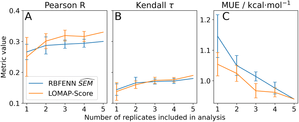Fig. 10 Statistical performances of RBFE predictions on the TNKS2 RBFE benchmarking series versus experimental ligand binding affinities using the data-driven approach described in this work (RBFENN; blue) versus the state-of-the-art LOMAP-Score approach (orange) for various statistical metrics. The data is presented as a dynamic representation of replicate inclusion, where for each progression of x all possible combinations of replicates (n = x) are included for the calculation of the mean metric value. Depicted error bars show the standard error of the mean metric across replicates; as for 5 replicates there is only one combination (all replicates), no confidence has been depicted.

The dynamic representation of statistical performances across replicates for TNKS2 highlights the importance of assessing protocol repeatability.^60,61 It appears that none of the statistical metrics have fully reached a plateau after 5 repeats, suggesting that the RBFE protocol could benefit from an even larger number of replicates or other optimisations. Although in this analysis no reference can be made to an optimal network chosen according to |ΔΔG_offset| values as in Section 3.3.4, the RBFENN (28 edges) and LOMAP-Score (27 edges) networks can be directly compared. With an overlap of 27%, the overlap is considerably lower than with TYK2. The eight shared edges are predominantly single-atom perturbations. The main observed qualitative difference between the two networks is in how either handles the alkyl-OH motifs and the (de)halogenations: it appears that in general the LOMAP-Score network allocates more edges to (de)halogenations (e.g.5k → 5m → 5i Fig. S18†), whereas the RBFENN network focuses more on allocating edges to perturbing the alkyl-OH motifs (e.g.5o → 5p → 5i, Fig. S17†). This coincides with a recent observation by Cresset developers that the default simulation protocol for SOMD fared poorly for perturbation involving alkyl-OH motifs. This has been subsequently corrected by tuning softcore parameters. These new parameter settings have not been used for the generation of the current version of RBFE-Space which explains the behaviour of the data-driven approach in this analysis.

Although the main aim of the TNKS2 screen was to compare directly the performances between RBFENN and LOMAP-Score networks, SOMD performance on TNKS2 in this work is poor compared to results published elsewhere. For example, Schindler et al.¹⁵ and Gapsys et al.¹⁶ report MUE values of 0.62 and 0.73 kcal mol⁻¹, respectively. Note that these values were computed using edges on neutral ligands only. Both of these examples contained considerably larger RBFE networks (45 edges); Schindler et al. note that these were obtained by requesting an optimal topology from the FEP+ implementation and no manual network augmentation was performed. This suggests that increased performance could be have been achieved using networks with a greater number of edges. Indeed, in-house results from Cresset suggest that Flare FEP (which deploys SOMD as its back-end RBFE engine) outperforms per-ligand binding affinity predictions of Schindler et al. with a manually adjusted network (70 edges), giving a MUE of 0.60 kcal mol⁻¹ and a pearson R value of 0.75 (Tables S1 and S2†).

4 Conclusions

In RBFE network generation there exist two main challenges: estimating the reliability of RBFE perturbations that form the edge of a network a priori, and optimising resources allocation to process a network that spans all compounds. The current work describes research into the first problem. Investigations into optimal network topology are actively being carried out.^21,25,26 Because the accuracy of an RBFE protocol is sensibly affected by the choice of the perturbation network this has important implications for the field. For instance, forcefield benchmarking studies with a given RBFE implementation should ideally be carried out with the same perturbation network. Benchmarking studies of different RBFE implementations should be made with networks tuned for performance for each implementation.

This work introduces several new concepts to the field of RBFE. By grafting a large number of RBFE perturbations onto a common benzene scaffold, a transferable training set was created for RBFE research and development. As this set covers a diverse set of RBFE perturbations it is highly suitable for ML work and is set to drive research in combining RBFE and ML methodologies further. A future direction for RBFESpace would be to explore whether the SEM of a large perturbation could be estimated from the SEMs of simpler sub-perturbations. This could allow increasing the size of the training set without increasing computing cost.

Using a siamese neural network architecture with graph representation of RBFE endpoint ligands, a SEM predictor was trained on RBFE-Space. This predictor is shown to outperform state-of-the-art heuristics in the context of modelling statistical uncertainties. The prototype predictor (RBFENN) was used to generate the first ML-based networks for planning of RBFE calculations. A future iteration of RBFENN could focus on optimisation of the data augmentation stage used in the pre-training stage since the current approach introduces correlations between data points that could influence the subsequent transfer learning step.

The prototype data-driven network generators are shown to match performance of state-of-the-art rule-based RBFE network generators that have required extensive calibration over multiple years to perform adequately with specific RBFE implementations. By contrast the data-driven method offers full transferability to other RBFE implementations with the single requirement of running a set of prescribed RBFE-Space simulations to recreate SEM values specific to that implementation. Beside network generation, the RBFENN predictor presented in this work could be used to ‘boostrap’ adaptive sampling schemes for initial resources allocation, for instance the NetBFE algorithm.²⁶ Our work has focused on normalising predicted SEM values into a LOMAP-Score metric for the LOMAP algorithm. Other algorithms based on optimal design principles could use RBFENN estimates to construct networks that minimise the total expected variance.^25,50 The availability of an inexpensive predictor of SEMs could also be exploited by algorithms that sample chemical space to identify molecules whose RBFE reliability to a reference compound can be determined with ease.

A promising application of the approach presented in this work is its implementation into an optimal design approach that aims to minimise the expected variance such as NetBFE.²⁶ Using these predicted variance, these types of network planning algorithms could be seeded with initial informed estimations of variances in the network which could accelerate the optimal design algorithm. The current study has been built on a LOMAP-Style network planning algorithm largely because this is the current practice in our workflows - optimal design requirements such as specifying a priori the number of edges/the amount of sampling and implementing cycle closure methodologies was considered out of scope for this study, but could be explored in future work.

As all heuristics depicted in Table 2 attempt to model RBFE inaccuracy (in the form of e.g. |ΔΔG_offset| values), this begs the question as to whether a predictor can be trained directly on this quantity instead of precisions. For this, instead of grafting perturbations onto benzene (as with RBFE-Space), the original ligands must be featurised as well as the protein system in which the RBFE perturbation takes place. This has been attempted before and offers additional information such as pose differences between input ligands which are highly influential to the RBFE reliability.^27,28 However, the bottleneck in this scenario is that a large number of RBFE simulations must be run. Additionally robust experimental binding affinity must be available for each RBFE edge Indeed, during early investigations of this work attempts were made to create a training set that included original ligands, but the chemical space associated with training such a model appeared too large with respect to the data available. For example, the PDBbind v2020 database⁶² contains 19 443 protein-ligand complexes (with experimental binding affinities) across 5316 proteins. Assuming equal distribution of ligands per protein in this set brings the average size of congeneric series to . Mapping all edges in each network results in (3.6² − 3.6) × 5316 = 49, 758 RBFE calculations, which is still a (very) conservative estimate as it is likely that some series will be larger than others: the number of possible edges in each series scales O(n²). Alternatively, a retrospective dataset could be generated gradually using previously completed RBFE calculations. This in turn presents several challenges because each point in the dataset will need be standardised as in general RBFE protocols evolve over time (thus affecting the accuracy of the results for the same perturbation) and even within RBFE campaigns different edges may be allocated different degrees of sampling (e.g. different numbers of λ windows).

Alternatively models could be trained on datasets built using ΔΔG_bind SEM values (Fig. 5D and Table 2): this would at least remove the requirement of experimental binding free energies for each data point, opening up the possibility of manually curating the chemical space in order to construct a diverse dataset rather than being restricted to congeneric series that have experimental data. Additionally, an RBFE-Space version with original ligands (i.e. not grafted onto benzene) would enable faster predictions as this removes the need for additional MCS calculations to map ligands onto RBFE-Space abstractions. However, this method would still require simulations of the bound leg for each data point (to generate the training set) which could still be prohibitively expensive. Training on ΔG_solvated SEM values with original ligands is possible. However this space is still large due to chemical diversity of drug-like molecular scaffolds. We estimate that such dataset would require ∼2.5 M perturbations.

Another possible future direction is to pursue an active learning approach where the RBFENN is re-trained using newly-obtained |ΔΔG_offset| values for edges while a congeneric series is being explored in a live drug discovery project. This could be combined with an adaptive approach to tune simulation protocols (in effect allocating different sampling efforts) to individual network edges.

Overall this work has demonstrated the importance of perturbation network planning for RBFE calculations, and the potential of machine learning to automate the generation of optimal RBFE networks. Continued efforts in this direction will increase the robustness and effectiveness of RBFE methodologies for drug discovery.

Data availability

All python code and jupyter notebooks used in this work are made publicly available under a GPL-2.0 license at https://github.com/michellab/RBFENN.

Author contributions

J. S.: conceptualization, methodology, software, validation, formal analysis, investigation, data curation, writing – original draft, writing – review & editing, visualization M. M.: writing – review & editing, supervision J. M.: conceptualization, methodology, resources, formal analysis, writing – review & editing, supervision, project administration, funding acquisition.

Conflicts of interest

JM is a member of the Scientific Advisory Board of Cresset. MM owns shares in Cresset.

Acknowledgements

The Hartree Centre (JADE1&2), HecBioSim [EPSRC grant no EP/R029407/1] is acknowledged for supercomputer time in aid of running RBFE-Space simulations (2.1.2). The authors thank Lester Hedges for the continuous development of BioSimSpace and contributing to discussions relating to the current work's algorithms. The authors also thank Antonia Mey, Huafeng Xu and David Mobley for valuable exchanges of knowledge regarding RBFE network generation and the usage of algorithms they developed and Peter Cherry for providing results on the TNKS2 dataset run by Cresset.

Notes and references

1. K. A. Armacost, S. Riniker and Z. Cournia, J. Chem. Inf. Model., 2020, 60, 1–5.
2. B. Kuhn, M. Tichý, L. Wang, S. Robinson, R. E. Martin, A. Kuglstatter, J. Benz, M. Giroud, T. Schirmeister, R. Abel, F. Diederich and J. Hert, J. Med. Chem., 2017, 60, 2485–2497.
3. Z. Cournia, B. Allen and W. Sherman, J. Chem. Inf. Model., 2017, 57, 2911–2937.
4. A. D. Simone, C. Georgiou, H. Ioannidis, A. A. Gupta, J. Juárez-Jiménez, D. Doughty-Shenton, E. A. Blackburn, M. A. Wear, J. P. Richards, P. N. Barlow, N. Carragher, M. D. Walkinshaw, A. N. Hulme and J. Michel, Chem. Sci., 2019, 10, 542–547.
5. Y. Khalak, G. Tresadern, M. Aldeghi, H. M. Baumann, D. L. Mobley, B. L. de Groot and V. Gapsys, Chem. Sci., 2021, 12, 13958–13971.
6. C. Mendoza-Martinez, M. Papadourakis, S. Llabrés, A. A. Gupta, P. N. Barlow and J. Michel, Chem. Sci., 2022, 13, 5220–5229.
7. S. Bosisio, A. S. J. S. Mey and J. Michel, J. Comput.-Aided Mol. Des., 2016, 31, 61–70.
8. A. Rizzi, T. Jensen, D. R. Slochower, M. Aldeghi, V. Gapsys, D. Ntekoumes, S. Bosisio, M. Papadourakis, N. M. Henriksen, B. L. de Groot, Z. Cournia, A. Dickson, J. Michel, M. K. Gilson, M. R. Shirts, D. L. Mobley and J. D. Chodera, J. Comput.-Aided Mol. Des., 2020, 34, 601–633.
9. G. J. Rocklin, S. E. Boyce, M. Fischer, I. Fish, D. L. Mobley, B. K. Shoichet and K. A. Dill, J. Mol. Biol., 2013, 425, 4569–4583.
10. H. H. Loeffler, S. Bosisio, G. D. R. Matos, D. Suh, B. Roux, D. L. Mobley and J. Michel, J. Chem. Theory Comput., 2018, 14, 5567–5582.
11. Y. Qiu, D. G. A. Smith, S. Boothroyd, H. Jang, D. F. Hahn, J. Wagner, C. C. Bannan, T. Gokey, V. T. Lim, C. D. Stern, A. Rizzi, B. Tjanaka, G. Tresadern, X. Lucas, M. R. Shirts, M. K. Gilson, J. D. Chodera, C. I. Bayly, D. L. Mobley and L.-P. Wang, J. Chem. Theory Comput., 2021, 17, 6262–6280.
12. L. Wang, Y. Wu, Y. Deng, B. Kim, L. Pierce, G. Krilov, D. Lupyan, S. Robinson, M. K. Dahlgren, J. Greenwood, D. L. Romero, C. Masse, J. L. Knight, T. Steinbrecher, T. Beuming, W. Damm, E. Harder, W. Sherman, M. Brewer, R. Wester, M. Murcko, L. Frye, R. Farid, T. Lin, D. L. Mobley, W. L. Jorgensen, B. J. Berne, R. A. Friesner and R. Abel, J. Am. Chem. Soc., 2015, 137, 2695–2703.
13. D. F. Hahn, C. I. Bayly, H. E. B. Macdonald, J. D. Chodera, V. Gapsys, A. S. J. S. Mey, D. L. Mobley, L. P. Benito, C. E. M. Schindler, G. Tresadern and G. L. Warren, Best practices for constructing, preparing, and evaluating protein-ligand binding affinity benchmarks, 2021, https://arxiv.org/abs/2105.06222.
14. A. S. J. S. Mey, B. K. Allen, H. E. Bruce McDonald, J. D. Chodera, D. F. Hahn, M. Kuhn, J. Michel, D. L. Mobley, L. N. Naden, S. Prasad, A. Rizzi, J. Scheen, M. R. Shirts, G. Tresadern and H. Xu, J. Open Source Softw., 2020, 2, 18378.
15. C. E. M. Schindler, H. Baumann, A. Blum, D. Böse, H.-P. Buchstaller, L. Burgdorf, D. Cappel, E. Chekler, P. Czodrowski, D. Dorsch, M. K. I. Eguida, B. Follows, T. Fuchß, U. Grädler, J. Gunera, T. Johnson, C. Jorand Lebrun, S. Karra, M. Klein, T. Knehans, L. Koetzner, M. Krier, M. Leiendecker, B. Leuthner, L. Li, I. Mochalkin, D. Musil, C. Neagu, F. Rippmann, K. Schiemann, R. Schulz, T. Steinbrecher, E.-M. Tanzer, A. Unzue Lopez, A. Viacava Follis, A. Wegener and D. Kuhn, J. Chem. Inf. Model., 2020, 60, 5457–5474.
16. V. Gapsys, D. F. Hahn, G. Tresadern, D. L. Mobley, M. Rampp and B. L. de Groot, J. Chem. Inf. Model., 2022, 62, 1172–1177.
17. A. S. J. S. Mey, J. J. Jiménez and J. Michel, J. Comput.-Aided Mol. Des., 2017, 32, 199–210.
18. M. M. Reif and C. Oostenbrink, J. Comput. Chem., 2013, 35, 227–243.
19. D. R. Slochower, N. M. Henriksen, L.-P. Wang, J. D. Chodera, D. L. Mobley and M. K. Gilson, J. Chem. Theory Comput., 2019, 15, 6225–6242.
20. J. A. Maier, C. Martinez, K. Kasavajhala, L. Wickstrom, K. E. Hauser and C. Simmerling, J. Chem. Theory Comput., 2015, 11, 3696–3713.
21. Q. Yang, W. Burchett, G. S. Steeno, S. Liu, M. Yang, D. L. Mobley and X. Hou, J. Comput. Chem., 2020, 41, 247–257.
22. S. Liu, Y. Wu, T. Lin, R. Abel, J. P. Redmann, C. M. Summa, V. R. Jaber, N. M. Lim and D. L. Mobley, J. Comput.-Aided Mol. Des., 2013, 27, 755–770.
23. M. Kuhn, S. Firth-Clark, P. Tosco, A. S. J. S. Mey, M. Mackey and J. Michel, J. Chem. Inf. Model., 2020, 60, 3120–3130.
24. Flare, https://www.cresset-group.com/tag/flare/.
25. H. Xu, J. Chem. Inf. Model., 2019, 59, 4720–4728.
26. P. Li, Z. Li, Y. Wang, H. Dou, B. K. Radak, B. K. Allen, W. Sherman and H. Xu, J. Chem. Theory Comput., 2022, 18, 650–663.
27. J. Jiménez-Luna, L. Pérez-Benito, G. Martínez-Rosell, S. Sciabola, R. Torella, G. Tresadern and G. D. Fabritiis, Chem. Sci., 2019, 10, 10911–10918.
28. A. T. McNutt and D. R. Koes, J. Chem. Inf. Model., 2022, 62, 1819–1829.
29. J. Scheen, W. Wu, A. S. J. S. Mey, P. Tosco, M. Mackey and J. Michel, J. Chem. Inf. Model., 2020, 60, 5331–5339.
30. G. Landrum, Open-Source Cheminformatics Software, http://www.rdkit.org/.
31. G. Landrum, Molecule highlighting and R-group decomposition, 2020, http://rdkit.blogspot.com/2020/10/molecule-highlighting-and-r-group.html.
32. P. Schmidtke, Grafting fragments onto molecules in rdkit – babysteps, 2021, https://pschmidtke.github.io/blog/rdkit/3d-editor/2021/01/23/grafting-fragments.html.
33. L. Hedges, A. Mey, C. Laughton, F. Gervasio, A. Mulholland, C. Woods and J. Michel, J. Open Source Softw., 2019, 4, 1831.
34. G. Calabrò, C. J. Woods, F. Powlesland, A. S. J. S. Mey, A. J. Mulholland and J. Michel, J. Phys. Chem. B, 2016, 120, 5340–5350.
35. C. Woods, A. S. J. S. Mey, G. Calabrò and J. Michel, Sire Molecular Simulation Framework, 2019.
36. M. R. Shirts and J. D. Chodera, J. Chem. Phys., 2008, 129, 124105.
37. D. Chicco, in Siamese Neural Networks: An Overview, ed. H. Cartwright, Springer US, New York, NY, 2021, pp. 73–94.
38. G. Koch, R. Zemel and R. Salakhutdinov, Siamese Neural Networks for One-shot Image Recognition, W&CP, vol. 37, 2015.
39. J. Gilmer, S. S. Schoenholz, P. F. Riley, O. Vinyals and G. E. Dahl, Proceedings of the 34th International Conference on Machine Learning, vol 70, 2017, pp. 1263–1272.
40. B. Ramsundar, P. Eastman, P. Walters, V. Pande, K. Leswing and Z. Wu, Deep Learning for the Life Sciences, O'Reilly Media, 2019.
41. A. Kensert, Keras documentation: Message-passing neural network for molecular property prediction, 2021, https://keras.io/examples/graph/mpnn-molecular-graphs/.
42. F. Zhuang, Z. Qi, K. Duan, D. Xi, Y. Zhu, H. Zhu, H. Xiong and Q. He, A Comprehensive Survey on Transfer Learning, 2019, https://arxiv.org/abs/1911.02685.
43. J. S. Delaney, J. Chem. Inf. Comput. Sci., 2004, 44, 1000–1005.
44. P. Walters, 2018, http://practicalcheminformatics.blogspot.com/2018/09/predicting-aqueous-solubility-its.html.
45. G. B. Goh, C. Siegel, A. Vishnu and N. O. Hodas, Using Rule-Based Labels for Weak Supervised Learning: A ChemNet for Transferable Chemical Property Prediction, 2018.
46. X. Li and D. Fourches, Inductive transfer learning for molecular activity prediction: Next-Gen QSAR Models with MolPMoFiT, 2020, https://jcheminf.biomedcentral.com/articles/10.1186/s13321-020-00430-x#citeas.
47. H. Moriwaki, Y.-S. Tian, N. Kawashita and T. Takagi, J. Cheminf., 2018, 10, 4.
48. N. Schneider, D. M. Lowe, R. A. Sayle and G. A. Landrum, J. Chem. Inf. Model., 2015, 55, 39–53.
49. A. Mey, M. Mackey, P. Tosco, J. Scheen and J. Michel, Free Energy Network Analysis, https://github.com/michellab/freenrgworkflows/tree/devel.
50. Q. Yang, W. Burchett, G. S. Steeno, S. Liu, M. Yang, D. L. Mobley and X. Hou, J. Comput. Chem., 2020, 41(3), 247–257.
51. V. Fung, J. Zhang, E. Juarez and B. G. Sumpter, npj Comput. Mater., 2021, 7, 1.
52. D. Jiang, Z. Wu, C.-Y. Hsieh, G. Chen, B. Liao, Z. Wang, C. Shen, D. Cao, J. Wu and T. Hou, J. Cheminf., 2021, 13, 12.
53. Y. Wang, J. Wang, Z. Cao and A. B. Farimani, Nat. Mach. Intell., 2022, 4, 279–287.
54. C. W. Coley, W. Jin, L. Rogers, T. F. Jamison, T. S. Jaakkola, W. H. Green, R. Barzilay and K. F. Jensen, Chem. Sci., 2019, 10, 370–377.
55. C. Cai, S. Wang, Y. Xu, W. Zhang, K. Tang, Q. Ouyang, L. Lai and J. Pei, J. Med. Chem., 2020, 63, 8683–8694.
56. G. Pesciullesi, P. Schwaller, T. Laino and J.-L. Reymond, Nat. Commun., 2020, 11, 1.
57. D. A. Rufa, H. E. Bruce Macdonald, J. Fass, M. Wieder, P. B. Grinaway, A. E. Roitberg, O. Isayev and J. D. Chodera, bioRxiv, 2020, 227959.
58. K. M. Merz, J. Chem. Theory Comput., 2010, 6, 1769–1776.
59. L. Takács, J. Comb. Theory Ser. A., 1990, 53, 321–323.
60. B. Knapp, L. Ospina and C. M. Deane, J. Chem. Theory Comput., 2018, 14, 6127–6138.
61. A. Grossfield, P. N. Patrone, D. R. Roe, A. J. Schultz, D. Siderius and D. M. Zuckerman, J. Open Source Softw., 2019, 1, 1.
62. M. Su, Q. Yang, Y. Du, G. Feng, Z. Liu, Y. Li and R. Wang, J. Chem. Inf. Model., 2019, 59, 895–913.

---

Footnotes

† Electronic supplementary information (ESI) available. See DOI: https://doi.org/10.1039/d2dd00083k

‡ see e.g. commit e7026e671d7a410e220dc110ad79a0d661b30b8b at (https://github.com/MobleyLab/Lomap/).

---