Reorganization energies of flexible organic molecules as a challenging target for machine learning enhanced virtual screening

Abstract

The molecular reorganization energy λ strongly influences the charge carrier mobility of organic semiconductors and is therefore an important target for molecular design. Machine learning (ML) models generally have the potential to strongly accelerate this design process (e.g. in virtual screening studies) by providing fast and accurate estimates of molecular properties. While such models are well established for simple properties (e.g. the atomization energy), λ poses a significant challenge in this context. In this paper, we address the questions of how ML models for λ can be improved and what their benefit is in high-throughput virtual screening (HTVS) studies. We find that, while improved predictive accuracy can be obtained relative to a semiempirical baseline model, the improvement in molecular discovery is somewhat marginal. In particular, the ML enhanced screenings are more effective in identifying promising candidates but lead to a less diverse sample. We further use substructure analysis to derive a general design rule for organic molecules with low λ from the HTVS results.

---

I. Introduction

By providing fast and accurate predictions of molecular properties, chemical machine learning (ML) has the potential to significantly increase the speed and scope of molecular discovery.^1–3 In this context, much attention has been paid on properties that are directly available from single-point electronic structure (e.g. density functional theory, DFT) calculations, such as atomization energies^4–6 or molecular orbital energies.^7,8 For established benchmark sets of small molecules like QM9,⁹ state-of-the-art ML models now reach extremely high accuracies for such properties, often surpassing the intrinsic error of the reference electronic structure methods.

Despite this success, there remains a gap between the small, rigid molecules in QM9 and technologically or pharmaceutically relevant compounds, which are often larger and much more flexible. Furthermore, the target properties of molecular discovery are in practice seldom simple electronic properties that are directly accessible through single-point DFT calculations. Instead, complex properties like the bulk electronic conductivity, pharmacological or catalytic activity of a molecule are ultimately of interest.¹⁰ Unfortunately, these are extremely complicated to rigorously simulate even for a single molecule. In high-throughput virtual screening (HTVS) studies, it has therefore become common to focus on simplified descriptors that are known to correlate with the property of interest.^11–13 Such descriptors include, e.g., the binding energy of a key intermediate in catalysis or the internal reorganization energy (λ) in molecular electronics.

Measuring the energetic cost for charge-carriers to move between molecular sites,^14,15λ provides an important contribution to the charge-carrier mobility in crystalline and amorphous organic semiconductors.^16,17 While computational screening for low-λ molecular structures has successfully guided discovery,¹⁸ its sensitivity to small variations in molecular structure¹⁹ renders a targeted molecular design challenging. Fragment^19–21 or rule-based^22,23 design strategies have been proposed to tackle this problem, while virtual screening^24–29 or data-efficient^30,31 discovery were used to assess large molecular candidate spaces, albeit without fully capturing the underlying structure–property relationships.

A reliable ML-based prediction of λ could fill exactly this gap—providing significant speed-ups for the assessment of thousands of molecules while potentially allowing for the extraction of robust chemical rules by explainable AI.³² ML-based approaches were indeed recently successful for the prediction of λ for rigid molecules,³³ while flexible molecules still pose a significant challenge,³⁴ likely because λ simultaneously depends on two potential energy surfaces (see Fig. 1).

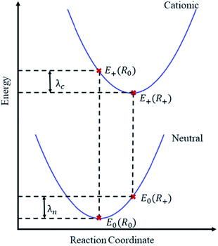Fig. 1 Illustration of the adiabatic potential energy surfaces of neutral and cationic molecular states. The reorganization energy λ is here calculated from the four indicated points³⁸ as λ = E₀(R₊) − E₀(R₀) + E₊(R₀) − E₊(R₊). Focusing on holes as charge carriers, E₀ and E₊ are the total energies of the neutral and cationic molecular states, evaluated at the equilibrium geometries R₀ and R₊ of the respective states. In practice, two equilibrium geometries thus need to be obtained.

In this contribution we therefore critically study the ML prediction of λ (specifically for hole conduction) as a challenging problem for chemical machine learning. To this end, we present a new dataset of hybrid DFT-level reorganization energies for 10 900 carbon and hydrogen containing molecules consisting of up to sixty atoms and five rotatable bonds. A series of Gaussian Process Regression (GPR)^35,36 models are developed for this dataset, both for straightforward structure/property mapping and Δ-ML³⁷ using a semiempirical baseline. We find that the conformational freedom of these molecules can introduce significant noise to this inference task, so that the performance of the models is strongly influenced by the conformer sampling method. We further show that significant improvements in the predictive performance are achieved by adopting the Δ-learning strategy. Finally, we critically evaluate the usefulness of the obtained ML methods for the discovery of low-λ structures in a diverse chemical space and for deducing molecular design rules.

II. Methods

Dataset

A set of flexible π-conjugated hydrocarbon molecules was generated by successively applying a series of molecular transformation operations to benzene (see Fig. S1†), similar to the procedure used in ref. 30. At each step, these operations modify structural elements in the parent molecule or add additional ones. The set of operations used herein includes biphenyl-conjugation, annelation (5/6-ring) and ring-contraction, among others (see ESI† for details). Based on these transformations, molecular structures with up to four rings and two linker atoms were randomly generated, leading to 131 810 unique structures. This set forms the virtual screening space for this study. DFT calculations were performed for a subset of 10 900 structures as detailed in the section on Structure-based ML models.

While these molecules thus purposely cover a diverse molecular and conformational space, we note that—as with any enumerated chemical dataset—unstable and reactive systems could be contained and synthesizability should be assessed separately. All chemoinformatics-related tasks were carried out using RDKit 2019.09.03.³⁹

Reorganization energies

Reorganization energies were calculated for the lowest-energy conformer of each molecule. To determine this conformer, RDKit is first used to compute 2D coordinates for the molecular graph, while an initial 3D structural guess is obtained and relaxed at the GFN2-xTB level using the xTB program (v6.3.0).⁴⁰ Conformational search is then carried out using the iterative meta-dynamics sampling and genetic crossover (iMTD-GC) approach, as implemented in the “Conformer-Rotamer Ensemble Sampling Tool” (CREST).⁴¹ Here, three different settings were compared as fully detailed in the Results section.

For the lowest-energy conformers, reorganization energies were computed at the GFN1-xTB level (λ_GFN1). Note that GFN1-xTB was chosen instead of its successor (GFN2-xTB) because we found the former to be slightly more reliable in terms of predicting λ and molecular geometries for the systems considered herein (see Fig. S2 and S3†). Electronic descriptor values entering property-based ML models (as detailed in the Results section) were also extracted from results of these calculations. These include frontier orbital energies and their gaps, Fermi levels, total energies and vertical energy differences. Final target λ_DFT values were calculated at the B3LYP^42–44 level of theory using the FHI-AIMS⁴⁵ code, including the TS dispersion correction.⁴⁶ Electronic wave functions were expanded in an extended “tier 1” basis set using “light” integration settings. Note that this level of theory is commonly employed for characterizing organic semiconductors, thus forming a good reference method for this study.^19,25,28,47

ML models

All models presented herein use GPR, a probabilistic machine learning method that allows for the smooth interpolation of property values from data. Specifically, these models infer the underlying relationship between different molecular representations and λ, based on a training set D = {X, y}. Here, X is a matrix consisting of molecular representation vectors x⁽ⁱ⁾ and y is a vector of target properties for the training molecules, with elements y⁽ⁱ⁾. Predictions for a set of unseen molecular representations X* can then be obtained as the predictive mean

ȳ(X*) = αK(X*, X), (1)

where the covariance (or kernel) matrix K with elements K_ij = K(x⁽ⁱ⁾, x^(j)) quantifies the similarity between molecular representations. The coefficients α minimize a regularized least-squares error between property predictions and reference values and can be calculated as

α = (K(X, X) + σ_n²1)⁻¹y (2)

where K(X, X) is again a covariance matrix. The hyperparameter σ_n incorporates observation noise, in this case, e.g. related to uncertainty due to conformational sampling (as detailed in the section on Conformer sampling).

In all models reported herein, the commonly used radial basis function (RBF) kernel is employed:

where the l is the kernel length-scale, σ_f² is the signal variance and d(., .) is the Euclidean distance.

A series of GPR models are presented herein, which differ in the type of representation and in how the covariance matrix is constructed. The most straightforward of these uses a representation of the molecular geometry of the lowest-energy conformer in the neutral charge state. This representation x⁽ⁱ⁾_s is constructed in two steps. First, each atomic environment is encoded into a rotationally invariant local representation using the smooth overlap of atomic positions (SOAP)⁴⁸ as implemented in Dscribe⁴⁹ (see Fig. S4† for details). These atomic representations are then combined into molecular representations using the auto-bag method,⁵⁰ which partitions the local feature vectors into k_max clusters using the k-means algorithm.⁵¹ Each molecular structure can then be encoded by a k_max-dimensional global feature vector that counts the occurrence of local environments that are assigned to each cluster. The effect of the hyperparameter k_max on the predictive performance is shown in Fig. S5,† arriving at a converged value of 500. Here, SOAP is only one of the possible choices for representing atomic environments. In fact, there is a range of modern many-body representations, which are closely related to each other and typically display comparable accuracy.⁵² To illustrate this we also considered the Many-Body Tensor Representation of Huo and Rupp.⁵³ This indeed yields very similar predictive performance for structure based models (see Fig. S6†).

Note that above we introduced the subscript s to refer to the use of structure-based molecular representations and the corresponding baseline ML model is denoted with K_s. Furthermore, a model termed K_p based on electronic properties computed at the semiempirical GFN1-xTB level was developed, with the corresponding representation x⁽ⁱ⁾_p (see below for details). Finally, a model K_sp is explored, that combines the two kernel functions as K_sp(i,j) = K_s(x⁽ⁱ⁾_s,x^(j)_s) + K_p(x⁽ⁱ⁾_p,x^(j)_p).

The hyperparameters θ_s = (σ_fs, l_s, σ_n), θ_p = (σ_fp, l_p, σ_n), and θ_sp = (σ_fs, σ_fp, l_s, l_p, σ_n) for the respective models are determined by maximizing their log-marginal likelihood over D using the L-BFGS algorithm with randomly sampled initial values. Our custom GPR model is based on respective code from the scikit-learn⁵⁴ implementation.

It should be noted that the choice of the ML method can in principle have a strong influence on the predictive accuracy. For the case of molecular reorganization energies, Abarbanel and Hutchison therefore performed an extensive comparison of different regression approaches (e.g. using kernel, decision tree and neural network based methods), finding little difference between different ML approaches.³⁴ To confirm this insensitivity, we also trained a decision tree based AdaBoost⁵⁵ model on the current data set and indeed found little difference to the GPR approach used herein (see Fig. S7†).

III. Results

Conformer sampling

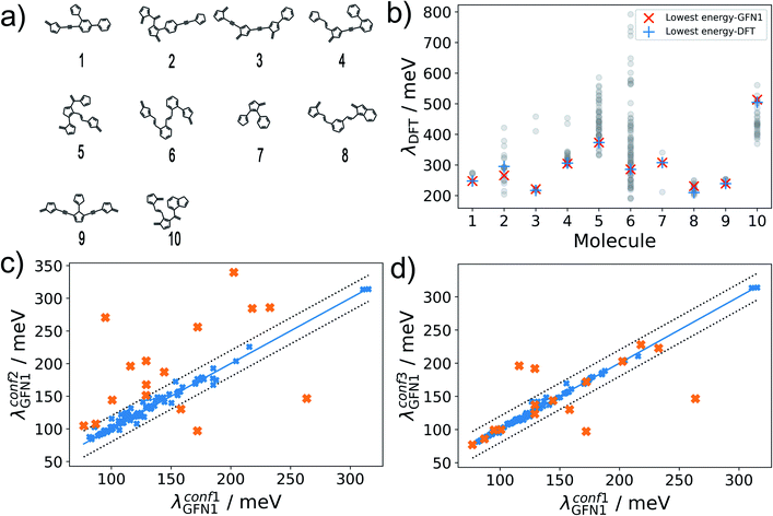
The hydrocarbon dataset presented herein contains molecules with diverse structural elements (see Fig. 2a for 10 randomly selected examples). While the enumerated 2D molecular graphs contain information on molecular bonding, they do not fully determine the molecular geometry, e.g. with respect to relative configurations around rotatable single bonds. As an example, 115 888 (53 046) of the contained molecules incorporate at least 2 (4) rotatable bonds, with a maximum of 5 rotatable bonds occurring overall. We thus expect a significant conformational flexibility for these molecules.

Fig. 2 Conformational diversity of the dataset. (a) Random molecules contained in the dataset. (b) Variability of λ_DFT obtained for full conformer ensembles derived from conf1 searches. Respective values obtained for the lowest-energy DFT or GFN1-xTB conformers are marked. (c) Correlation between λ_GFN1 for the lowest energy conformers obtained by with conf1 and conf2. Outliers are marked in orange. (d) Improved correlation is obtained for conf3, while outliers of (c) are again marked in orange.

This flexibility can influence the ML predictions of λ in two ways. First, the reference λ values may depend on the conformer, and flexible molecules display much larger conformational variety. Second, the ML prediction of λ is based on a representation derived from a 3D molecular geometry. For highly flexible molecules, we can expect significantly larger deviations between the geometries predicted with more approximate levels of theory and high-level references. This is known to impact the accuracy of ML models adversely.⁵⁶ To arrive at an internally consistent procedure when comparing among different molecular systems, we therefore focus on the lowest energy conformers that we can identify for each molecular system.

Unfortunately, a full conformer search at the DFT level is prohibitively expensive. This means that we require a robust and efficient protocol for the search of low-energy conformers. To this end we rely on semiempirical and force-field methods from the GFN family, which have recently been established for this purpose. These are used in combination with CREST, which implements a purpose-built workflow for conformational search.⁴¹ Depending on the underlying energy function, the accuracy and computational cost of this search can vary significantly, however. We therefore tested three different workflows, denoted as conf1-3.

In our reference method (conf1), we employ CREST in combination with the density functional tight-binding method GFN1-xTB.⁴⁰ Performing conformer searches for the 10 molecules of Fig. 2a, we find that between 3 and 90 conformers are identified within the default energy window of 6 kcal mol⁻¹ (260 meV) above the lowest energy one, underscoring the conformational flexibility of molecules in our dataset. For these conformer ensembles, we show the wide range of encountered λ_DFT values in Fig. 2b. Importantly, there is little variation between the values of λ_DFT calculated for the lowest-energy conformers at the GFN1-xTB and DFT level, which suggests that GFN1-xTB conformers are a reliable proxy for the true first-principles ground state geometry. Note that the excellent agreement in Fig. 2b only reflects the quality of GFN1-xTB conformers, while all reorganization energies in this subfigure were calculated at the DFT level. Unfortunately, performing the full conformer search at the GFN1-xTB level is still computationally prohibitive for hundreds of thousands of molecules, however.

Alternatively, the significantly more efficient force-field method GFN-FF⁵⁷ can be used, and the conformer search be accelerated using the ‘quick’ setting in CREST (herein termed conf2). For 100 randomly selected molecules, Fig. 2c shows a comparison of λ_GFN1 values for the lowest-energy conformers obtained with conf1 and conf2. While the bulk of the predictions falls within the error margins of ±20 meV, we also find 16 outliers – marked in orange. These can be attributed to an incomplete coverage of conformational space in the conf2 ensemble and to differences in the energetic ranking between GFN1-xTB and GFN-FF.

To address the latter point, in conf3 we therefore combine the higher accuracy of GFN1-xTB and the computational speed of GFN-FF: a conformer ensemble is generated with CREST at the GFN-FF level, while a subsequent local relaxation and energetic re-ranking is carried out using GFN1-xTB. Comparing again to conf1, we see a significantly better agreement between the methods (see Fig. 2d), with 5 remaining outliers falling beyond the error margins of ±20 meV. It should be noted, that conformer searches are in general a difficult global optimization problem, which cannot be solved deterministically in an efficient manner. Therefore, some amount of uncertainty is unavoidable and will affect the ML models in all cases. As discussed in the following, achieving lower uncertainty at this stage leads to significantly lower predictive errors, however.

Structure-based ML models

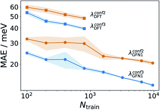
Having established an efficient conformer search workflow, we now turn to structure based ML models for predicting λ (K_s). As these models require 3D geometries as inputs, they are well suited to investigate the effect of the conformer search protocols on the ML models themselves, see Fig. 3. Here, learning curves for λ_GFN1 and λ_DFT are shown. While all models improve with more data, two striking differences can be seen. First, the models using the more accurate conformer search conf3 are consistently better than the ones using conf2. Second, the predictive error is consistently lower for λ_GFN1 than for λ_DFT.

Fig. 3 Effect of improved conformer searches on learning behavior. Learning curves for λ_DFT and λ_GFN1 using the conf2 and conf3 conformer search protocols. Training sets for λ_GFN1 (λ_DFT) consist of up to 9900 (880) molecules, with 1000 (100) unseen data points used to evaluate the predictive errors. Shaded errors indicate the standard deviation for five randomly draw training sets of each size. Note that the DFT assessment was stopped earlier due to the significantly higher computational cost of the method.

In part, this can be explained by the smaller range of λ_GFN1 values (see next section). However, a fundamental difference between the two targets also exists: While we predict λ_GFN1 on the basis of the corresponding neutral state molecular equilibrium structures, this does not hold for λ_DFT. In, the latter case, the differing neutral state equilibrium geometries (between GFN1-xTB and DFT) further complicate the learning task.

It should be noted here that learning λ_GFN1 is itself only of methodological interest, however. Indeed, the conf3 search requires GFN1-xTB for energy ranking, which has a similar computational effort to calculating λ_GFN1. In the following, we therefore exclusively focus on predicting λ_DFT, using conf3 for structure generation. To this end we extended our DFT annotated dataset to cover in total 10 900 molecules, randomly drawn from the full hydrocarbon database. The distribution of obtained λ_DFT values is shown in Fig. S8.† 1000 molecules served as an external test set for model validation, while at maximum 9600 of the remaining 9900 entered the respective training sets.

Beyond structure-based models

While the above results show that λ_DFT can be learned from the structure, the accuracy of the models leaves something to be desired, given that the intrinsic standard deviation of the dataset is ca. 80 meV. To explore how this performance is impacted by molecular flexibility, additional ΔK_s models were trained on different subsets of 1000 molecules with a fixed number of rotatable bonds (N_rb = 2,3,4,5). These models were then evaluated on test sets with the corresponding N_rb (see Fig. S9†). We find that models for less flexible molecules are indeed significantly more accurate than those for more flexible molecules. This confirms the notion that molecular flexibility poses a challenge for molecular ML models and underscores our previous point on the highly challenging nature of λ as a target property, e.g. compared to the atomization energy.

Since robust models already require the use of GFN1-xTB for conformer ranking, it is natural to ask whether electronic properties at the GFN1-xTB level could be used to improve them. The most straightforward way to do this is via a Δ-learning³⁷ strategy, i.e. by learning a correction to λ_GFN1. To this end, we first use a simple linear regression to describe systematic differences between λ_DFT and λ_GFN1:

λ_lin = aλ_GFN1 + b (4)

This linear model alone yields a stable MAE of 40 meV, independent of the training set size. It thus outperforms the structure based K_s models for all but the largest training sets (see Fig. 4). This means that, contrary to the findings of ref. 34 we find a reasonably good correlation between GFN and DFT based reorganization energies (R² = 0.54, see Fig. S10†). This is likely due to the different class of molecules (thiophene oligomers) considered therein. Defining as a new target property:

λ_Δ = λ_DFT − λ_lin, (5)

we can now build Δ-learning models that further improve on the linear approach. As expected, the Δ-learning variant of K_s (termed ΔK_s) indeed performs significantly better than both the linear and the baseline model, approaching an MAE of 30 meV at the largest training set size.

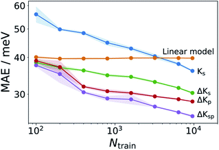Fig. 4 Learning curves for various ML models. Comparison of K_s models with various Δ-learning approaches. Shadings analogous to Fig. 3. The K_s model corresponds to the curve labeled λ^conf3_DFT in that figure.

The GFN1-xTB calculations required for obtaining λ_GFN1 can also be exploited in a different way. One challenge for the structure-based models is the indirect relationship between the neutral GFN1-xTB geometry and λ_DFT. We therefore also explored property-based models (termed K_p) which use frontier orbital energies and gaps, Fermi levels, total energies and vertical energy differences of the neutral and cationic system to construct a representation, as fully detailed in Table S2.† The respective ΔK_p model is actually slightly better than the corresponding structure-based model ΔK_s, despite not including any structural information. Finally, a combined model incorporating the structural and property kernels (termed ΔK_sp), performs better still, reaching an MAE of 25 meV at the largest training set size.

Please note that no optimization of the feature selection was performed for the property based models, other than checking that there were no strong linear dependencies between different properties. However, a more systematic feature selection procedure can provide physical insight and potentially improve the models. To explore this, we performed permutational feature importance (PFI) analysis for the ΔK_p model (see Fig. S11†).⁵⁹ This indicates that some features are particularly relevant for the model, e.g. the HOMO energy of the cationic state in the neutral geometry, the Fermi energy of the neutral state in the cation geometry and the individual contributions to the GFN1 reorganization energy. Based on this, we constructed additional models which only used subsets of the most important features. However, these sparse models displayed somewhat worse performance than the full model, indicating that all features ultimately contribute to the prediction accuracy. Nonetheless, more sophisticated feature engineering (e.g. using recursive selection or nonlinear transformations) may be able to achieve better performance with sparse models.

ML-assisted virtual screening

So far, we have seen that in a Δ-ML setting, the presented GPR models can lead to a modest increase in predictive performance relative to a semiempirical baseline method. This raises the question of whether this improvement has a tangible effect on the results of a HTVS for low-λ_DFT molecules. To address this issue, we applied ΔK_s, ΔK_sp (each trained on 9600 molecules) and GFN1-xTB to screen 120 910 previously unseen molecules for promising candidates. For each model, we extracted 500 candidates with the lowest predicted λ and calculated their actual λ_DFT values.

As illustrated in Fig. 5a, all three methods are quite successful in identifying promising candidates: from the 500 selected systems, GFN1-xTB identifies 436 molecules that display λ_DFT < 200 meV, compared to the somewhat higher numbers for the ΔK_s and the ΔK_sp models (where 487 and 492 are respectively identified). Narrowing the range to λ_DFT < 140 meV, the ΔK_sp still performs best and identifies 251 structures, while the ΔK_s and the GFN1-xTB identify 217 and 118 such cases, respectively.

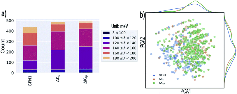Fig. 5 Results of the targeted identification of low-λ structures. (a) Distribution of λ_DFT values in the final selections derived from three different methods (see text). We only consider compounds that satisfy λ_DFT < 200 meV. (b) Kernel principal component analysis map of the identified structures (generated with the ASAP⁵⁸ code). Kernel-density estimates are shown along the principal components.

The 20 lowest-λ structures from all three screenings are shown in Fig. 6. Interestingly, 15 compounds in this subset were identified by the GFN1-xTB screening, while the ΔK_s and ΔK_sp models identified 9 and 11, falling slightly behind. In other words, the GFN1-xTB model actually has an edge over the ML model when considering the extreme low end of the distribution, although it is in general less effective in identifying low-λ structures. It is also notable that, although some overlap between the methods is observed (i.e. from the 1500 molecules selected by the three screenings only 1131 are unique candidates), many structures are exclusively identified by one method, in particular by GFN1-xTB. This is illustrated by the Kernel principal component analysis map⁵⁸ shown in Fig. 5b, which places similar molecular structures close to each other. Clearly, the semiempirical GFN1-xTB model overall exhibits the highest diversity, while the candidates selected by the data-driven models appear somewhat more concentrated. This reflects the fact that GPR models use metrics of molecular similarity in their predictions.

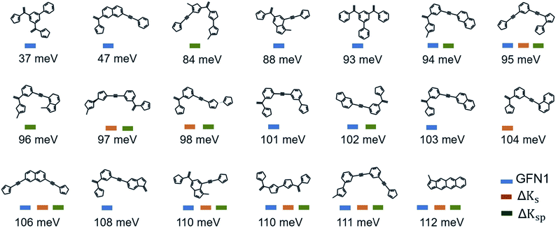Fig. 6 Lowest-λ_DFT candidates. Shown are the best candidates identified among 120k molecules in the three virtual screening campaigns. The corresponding λ_DFT values are listed below.

However, this is not primarily just a problem of the chosen models, since other ML approaches also (implicitly) work with feature similarity. It is rather that ML models are by definition most strongly influenced by those types of molecules which occur most frequently in the dataset. The HTVS setting does not necessarily require a good description of an average molecule, however. Instead, it requires a good description of the small percentage of unusual molecules that we are interested in. This implies that a non-uniform sampling strategy for training set construction might be helpful in this context. This will be explored in future work.

At the suggestion of a reviewer, the virtual screening was also performed with the ΔK_p approach (see Fig. S12 and S13†). This model shows comparable performance to ΔK_s for systems with λ < 140 meV, but is considerably worse for the range 140 meV < λ < 200 meV. This indicates that the structural information in ΔK_s and ΔK_sp helps the models to reliably identify systems that are structurally similar to low-λ training set molecules, thus increasing their screening accuracy.

Substructure analysis

Given a set of candidates from HTVS like the one in Fig. 6, it is natural to ask what makes these systems such good candidates. If general design rules could be obtained from this set, this would arguably be even more useful than the candidates themselves. Visual inspection indeed points to certain structural motifs that are fairly common, such as cyclopentadiene moieties and acetylene-bridged aromatic rings.

A more quantitative understanding of this can be obtained from a substructure analysis. To this end, we analysed whether certain structural motifs are significantly more likely to be found in the low-λ subset than in the full dataset. This can be quantified via the enrichment of a given substructure, defined as

where n_i,low and n_i,all are the number of times substructure i is found in the low-λ and full datasets, while N_low and N_all are the total number of molecules in each dataset. We complement this metric with the frequency of a given substructure in the dataset, defined as

f_i = (n_i,all/N_all). (7)

To obtain a general design rule, we search for substructures with both high enrichment and reasonably high frequency. This allows balancing between overly specific substructures that only occur in very few molecules to begin with (high enrichment/low frequency) and overly simple motifs that occur in many molecules, independent of λ (low enrichment/high frequency).

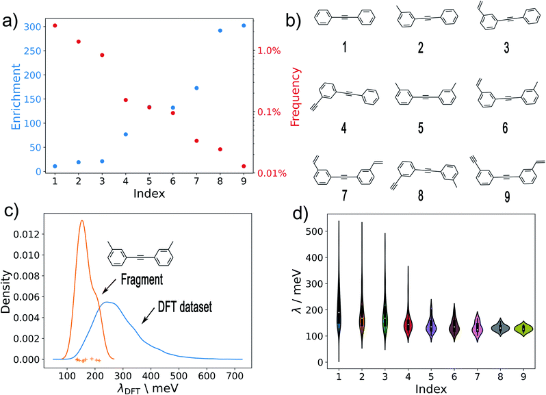
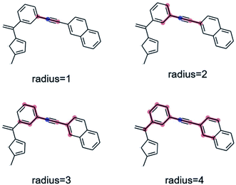
As a preliminary screening, potential substructures were defined via Morgan-fingerprints⁶⁰ of different bond-radii (see Fig. 8). As illustrated in Fig. S14,† this revealed a number of highly enriched substructures, which confirmed the initial impression that acetylene-bridged and cyclopentadiene containing structures are highly favourable. However, the substructures obtained in this fashion are often redundant and chemically unintuitive (i.e. by only containing parts of aromatic rings). We therefore manually derived a number of reasonable substructures from this analysis, in order to elucidate a robust and general design rule for low-λ molecules (see Fig. 7). Here, we focused on acetylene-bridged benzene rings, as cyclopentadiene is prone to dimerize in Diels–Alder reactions, pointing to potential stability issues with these molecules.

Fig. 7 Substructure analysis. (a) The enrichment and frequency of different substructures in the low-λ and full datasets, respectively. (b) Analysed substructures. (c) The kernel density estimated λ_DFT distributions of substructure 5 (shown in (b)) in the full training and validation sets (i.e. in 10 900 DFT datapoints). The individual λ-values of the ten molecules containing substructure 5 are shown as crosses. (d) Violin plots of λ_DFT for all substructures in all λ_DFT data.

Fig. 8 Graphical illustration of Morgan fingerprints with various radii. Fingerprints allow highlighting common structural motifs but also produce redundant results and may unintuitively cut through aromatic rings or functional groups.

In Fig. 7a, we plot the enrichment and frequency of each substructure. This reveals a contravening trend: The simplest structure (1) is very common in the full dataset, but also displays very low enrichment in the low-λ set. In contrast, the more elaborate structures (8) and (9) are highly enriched, but very rare overall. Meanwhile substructure (5) (two meta-substituted acetylene-bridged benzene rings) features a quite high enrichment and is also fairly common in the database. As a consequence, ten further molecules with this motif can be found in the previously computed set of 10 900 λ_DFT-values. This allows us to confirm that the corresponding molecules indeed display significantly lower reorganization energies than the full training set (Fig. 7c).

The distributions of λ_DFT-values for all substructures are shown in Fig. 7d. This confirms the impression obtained from the enrichment plots. Simple substructures like (1) are generally unspecific and can be found in both high- and low-λ molecules. Meanwhile, highly enriched substructures indeed robustly predict high quality candidates, and can thus be used to define general design rules.

It should be noted that the above analysis is ultimately limited by the biases of the underlying dataset. For example, heteroatomic substituents could affect the suitability of certain motifs quite strongly due to electronic push–pull effects, which are largely absent in the hydrocarbon dataset used herein. Nonetheless, the methodology we apply could of course also be applied to other datasets.

IV. Conclusion

In this work we have explored the potential benefits of using ML models to enhance virtual screening studies for molecules with low reorganization energies λ. We find that this is a challenging setting for molecular ML, both because of the conformational flexibility of the studied hydrocarbon molecules and the intrinsic difficulty of predicting λ from the equilibrium geometry alone. Both aspects can be mitigated by using a semiempirical electronic structure method for conformer searching and as a baseline model (provided there is at least a moderate correlation with the target property).

While this leads to a significant improvement of the predictive performance compared to the baseline, we find that the benefits of this are actually somewhat marginal in the context of virtual screening. Specifically, ML enhanced screening is more effective in identifying promising candidates, but the semiempirical model actually has some advantages in terms of candidate diversity. This calls into question whether the cost of building the ML models (in particular the generation of training data) is actually justified. In particular, computing λ_DFT for a single molecule takes on average 28 CPU hours on our hardware. In contrast, the generation of conformer ensembles (ca. 1 CPU hour per molecule) and the training of the ML models (one-time cost of 20 CPU hours for the largest training sets) are reasonably affordable. To obtain a clear advantage, more accurate and/or data-efficient ML models are thus required.

One way to achieve this would be to work with full conformer ensembles rather than single conformers to construct the representations.⁶¹ It should also be noted that packing and contact effects occurring in molecular crystals or amorphous structures are known to influence the encountered solid-state conformation and flexibility for geometrical relaxation.^26,62,63 Potentially, generative ML models trained on condensed phase data could therefore help producing more realistic conformer ensembles.

Data availability

Data and code for this paper is publicly available at https://gitlab.mpcdf.mpg.de/kchen/oscs.

Conflicts of interest

The authors declare no competing financial interests.

Acknowledgements

KC acknowledges funding from the China Scholarship Council. CK and JTM are grateful for support by Deutsche Forschungsgemeinschaft (DFG) through TUM International Graduate School of Science and Engineering (IGSSE), GSC 81. CK and KR gratefully acknowledge support from the Solar Technologies Go Hybrid initiative of the State of Bavaria. We also thankfully acknowledge computational resources provided by the Leibniz Supercomputing Centre.

References

1. K. T. Butler, D. W. Davies, H. Cartwright, O. Isayev and A. Walsh, Machine learning for molecular and materials science, Nature, 2018, 559, 547–555.
2. O. A. von Lilienfeld, K.-R. Müller and A. Tkatchenko, Exploring chemical compound space with quantum-based machine learning, Nat. Rev. Chem., 2020, 4, 347–358.
3. E. O. Pyzer-Knapp, K. Li and A. Aspuru-Guzik, Learning from the harvard clean energy project: the use of neural networks to accelerate materials discovery, Adv. Funct. Mater., 2015, 25, 6495–6502.
4. M. Rupp, A. Tkatchenko, K.-R. Müller and O. A. Von Lilienfeld, Fast and accurate modeling of molecular atomization energies with machine learning, Phys. Rev. Lett., 2012, 108, 058301.
5. G. Montavon, M. Rupp, V. Gobre, A. Vazquez-Mayagoitia, K. Hansen, A. Tkatchenko, K.-R. Müller and O. A. Von Lilienfeld, Machine learning of molecular electronic properties in chemical compound space, New J. Phys., 2013, 15, 095003.
6. H. Jung, S. Stocker, C. Kunkel, H. Oberhofer, B. Han, K. Reuter and J. T. Margraf, Size-extensive molecular machine learning with global representations, ChemSystemsChem, 2020, 2, e1900052.
7. A. Stuke, M. Todorović, M. Rupp, C. Kunkel, K. Ghosh, L. Himanen and P. Rinke, Chemical diversity in molecular orbital energy predictions with kernel ridge regression, J. Chem. Phys., 2019, 150, 204121.
8. M. Glavatskikh, J. Leguy, G. Hunault, T. Cauchy and B. Da Mota, Dataset's chemical diversity limits the generalizability of machine learning predictions, J. Cheminf., 2019, 11, 1–15.
9. R. Ramakrishnan, P. O. Dral, M. Rupp and O. A. von Lilienfeld, Quantum chemistry structures and properties of 134 kilo molecules, Sci. Data, 2014, 1, 1–7.
10. A. R. Thawani, R.-R. Griffiths, A. Jamasb, A. Bourached, P. Jones, W. McCorkindale, A. A. Aldrick, and A. A. Lee, The photoswitch dataset: a molecular machine learning benchmark for the advancement of synthetic chemistry, 2020, arXiv preprint arXiv:2008.03226.
11. J. Hachmann, R. Olivares-Amaya, S. Atahan-Evrenk, C. Amador-Bedolla, R. S. Sánchez-Carrera, A. Gold-Parker, L. Vogt, A. M. Brockway and A. Aspuru-Guzik, The harvard clean energy project: large-scale computational screening and design of organic photovoltaics on the world community grid, J. Phys. Chem. Lett., 2011, 2, 2241–2251.
12. E. O. Pyzer-Knapp, C. Suh, R. Gómez-Bombarelli, J. Aguilera-Iparraguirre and A. Aspuru-Guzik, What is high-throughput virtual screening? a perspective from organic materials discovery, Annu. Rev. Mater. Res., 2015, 45, 195–216.
13. Ö. H. Omar, M. del Cueto, T. Nematiaram and A. Troisi, High-throughput virtual screening for organic electronics: a comparative study of alternative strategies, J. Mater. Chem. C, 2021, 9, 13557–13583.
14. V. Coropceanu, J. Cornil, D. A. da Silva Filho, Y. Olivier, R. Silbey and J.-L. Bredas, Charge transport in organic semiconductors, Chem. Rev., 2007, 107, 926–952.
15. D. P. McMahon and A. Troisi, Evaluation of the external reorganization energy of polyacenes, J. Phys. Chem. Lett., 2010, 1, 941–946.
16. C. Wang, H. Dong, W. Hu, Y. Liu and D. Zhu, Semiconducting π-conjugated systems in field-effect transistors: a material odyssey of organic electronics, Chem. Rev., 2012, 112, 2208–2267.
17. J. Mei, Y. Diao, A. L. Appleton, L. Fang and Z. Bao, Integrated materials design of organic semiconductors for field-effect transistors, J. Am. Chem. Soc., 2013, 135, 6724–6746.
18. A. N. Sokolov, S. Atahan-Evrenk, R. Mondal, H. B. Akkerman, R. S. Sánchez-Carrera, S. Granados-Focil, J. Schrier, S. C. Mannsfeld, A. P. Zoombelt, Z. Bao and A. Aspuru-Guzik, From computational discovery to experimental characterization of a high hole mobility organic crystal, Nat. Commun., 2011, 2, 1–8.
19. H. Geng, Y. Niu, Q. Peng, Z. Shuai, V. Coropceanu and J.-L. Bredas, Theoretical study of substitution effects on molecular reorganization energy in organic semiconductors, J. Chem. Phys., 2011, 135, 104703.
20. C. Kunkel, C. Schober, J. T. Margraf, K. Reuter and H. Oberhofer, Finding the right bricks for molecular legos: A data mining approach to organic semiconductor design, Chem. Mater., 2019, 31, 969–978.
21. K.-H. Lin and C. Corminboeuf, Fb-reda: fragment-based decomposition analysis of the reorganization energy for organic semiconductors, Phys. Chem. Chem. Phys., 2020, 22, 11881–11890.
22. W.-C. Chen and I. Chao, Molecular orbital-based design of π-conjugated organic materials with small internal reorganization energy: generation of nonbonding character in frontier orbitals, J. Phys. Chem. C, 2014, 118, 20176–20183.
23. W. Huang, W. Xie, H. Huang, H. Zhang and H. Liu, Designing organic semiconductors with ultrasmall reorganization energies: insights from molecular symmetry, aromaticity and energy gap, J. Phys. Chem. Lett., 2020, 11, 4548–4553.
24. G. R. Hutchison, M. A. Ratner and T. J. Marks, Hopping transport in conductive heterocyclic oligomers: reorganization energies and substituent effects, J. Am. Chem. Soc., 2005, 127, 2339–2350.
25. M. Misra, D. Andrienko, B. Baumeier, J.-L. Faulon and O. A. von Lilienfeld, Toward quantitative structure-property relationships for charge transfer rates of polycyclic aromatic hydrocarbons, J. Chem. Theory Comput., 2011, 7, 2549–2555.
26. C. Schober, K. Reuter and H. Oberhofer, Virtual screening for high carrier mobility in organic semiconductors, J. Phys. Chem. Lett., 2016, 7, 3973–3977.
27. J. Yang, S. De, J. E. Campbell, S. Li, M. Ceriotti and G. M. Day, Large-scale computational screening of molecular organic semiconductors using crystal structure prediction, Chem. Mater., 2018, 30, 4361–4371.
28. E. Antono, N. N. Matsuzawa, J. Ling, J. E. Saal, H. Arai, M. Sasago and E. Fujii, Machine-learning guided quantum chemical and molecular dynamics calculations to design novel hole-conducting organic materials, J. Phys. Chem. A, 2020, 124, 8330–8340.
29. T. Nematiaram, D. Padula, A. Landi and A. Troisi, On the largest possible mobility of molecular semiconductors and how to achieve it, Adv. Funct. Mater., 2020, 30, 2001906.
30. C. Kunkel, J. T. Margraf, K. Chen, H. Oberhofer and K. Reuter, Active discovery of organic semiconductors, Nat. Commun., 2021, 12, 1–11.
31. C. Y. Cheng, J. E. Campbell and G. M. Day, Evolutionary chemical space exploration for functional materials: computational organic semiconductor discovery, Chem. Sci., 2020, 11, 4922–4933.
32. J. Jiménez-Luna, F. Grisoni and G. Schneider, Drug discovery with explainable artificial intelligence, Nat. Mach. Intell., 2020, 2, 573–584.
33. S. Atahan-Evrenk and F. B. Atalay, Prediction of intramolecular reorganization energy using machine learning, J. Phys. Chem. A, 2019, 123, 7855–7863.
34. O. Abarbanel and G. Hutchison, Machine learning to accelerate screening for marcus reorganization energies, J. Chem. Phys., 2021, 155, 054106.
35. C. Williams and C. Rasmussen, Gaussian processes for regression, in Advances in neural information processing systems, Max-Planck-Gesellschaft, MIT Press, Cambridge, MA, USA, 1996, pp. 514–520.
36. C. Rasmussen and C. Williams, Gaussian processes for machine learning, Adaptative computation and machine learning series, University Press Group Limited, 2006.
37. R. Ramakrishnan, P. O. Dral, M. Rupp and O. A. von Lilienfeld, Big data meets quantum chemistry approximations: The δ-machine learning approach, J. Chem. Theory Comput., 2015, 11, 2087–2096.
38. S. F. Nelsen, S. C. Blackstock and Y. Kim, Estimation of inner shell marcus terms for amino nitrogen compounds by molecular orbital calculations, J. Am. Chem. Soc., 1987, 109, 677–682.
39. The RDKit: Open-Source Cheminformatics Software, version 2019.09.3., 2019, http://www.rdkit.org.
40. S. Grimme, C. Bannwarth and P. Shushkov, A robust and accurate tight-binding quantum chemical method for structures, vibrational frequencies, and noncovalent interactions of large molecular systems parametrized for all spd-block elements (z = 1–86), J. Chem. Theory Comput., 2017, 13, 1989–2009.
41. P. Pracht, F. Bohle and S. Grimme, Automated exploration of the low-energy chemical space with fast quantum chemical methods, Phys. Chem. Chem. Phys., 2020, 22, 7169–7192.
42. A. D. Becke, Density-functional exchange-energy approximation with correct asymptotic behavior, Phys. Rev. A: At., Mol., Opt. Phys., 1988, 38, 3098.
43. C. Lee, W. Yang and R. G. Parr, Development of the colle-salvetti correlation-energy formula into a functional of the electron density, Phys. Rev. B: Condens. Matter Mater. Phys., 1988, 37, 785–789.
44. P. J. Stephens, F. J. Devlin, C. F. Chabalowski and M. J. Frisch, Ab initio calculation of vibrational absorption and circular dichroism spectra using density functional force fields, J. Phys. Chem., 1994, 98, 11623–11627.
45. V. Blum, R. Gehrke, F. Hanke, P. Havu, V. Havu, X. Ren, K. Reuter and M. Scheffler, Ab initio molecular simulations with numeric atom-centered orbitals, Comput. Phys. Commun., 2009, 180, 2175–2196.
46. A. Tkatchenko and M. Scheffler, Accurate molecular van der Waals interactions from ground-state electron density and free-atom reference data, Phys. Rev. Lett., 2009, 102, 073005.
47. N. E. Gruhn, D. A. da Silva Filho, T. G. Bill, M. Malagoli, V. Coropceanu, A. Kahn and J.-L. Bredas, The vibrational reorganization energy in pentacene: molecular influences on charge transport, J. Am. Chem. Soc., 2002, 124, 7918–7919.
48. A. P. Bartók, R. Kondor and G. Csányi, On representing chemical environments, Phys. Rev. B: Condens. Matter Mater. Phys., 2013, 87, 184115.
49. L. Himanen, M. O. Jäger, E. V. Morooka, F. F. Canova, Y. S. Ranawat, D. Z. Gao, P. Rinke and A. S. Foster, Dscribe: library of descriptors for machine learning in materials science, Comput. Phys. Commun., 2020, 247, 106949.
50. S. A. Meldgaard, E. L. Kolsbjerg and B. Hammer, Machine learning enhanced global optimization by clustering local environments to enable bundled atomic energies, J. Chem. Phys., 2018, 149, 134104.
51. S. Lloyd, Least squares quantization in pcm, IEEE Trans. Inf. Theory, 1982, 28, 129–137.
52. F. Musil, A. Grisafi, A. P. Bartók, C. Ortner, G. Csányi and M. Ceriotti, Physics-Inspired Structural Representations for Molecules and Materials, Chem. Rev., 2021, 121, 9759–9815.
53. H. Huo and M. Rupp, Unified Representation of Molecules and Crystals for Machine Learning, 2017, arXiv:1704.06439.
54. F. Pedregosa, G. Varoquaux, A. Gramfort, V. Michel, B. Thirion, O. Grisel, M. Blondel, P. Prettenhofer, R. Weiss, V. Dubourg, J. Vanderplas, A. Passos, D. Cournapeau, M. Brucher, M. Perrot and E. Duchesnay, Scikit-learn: Machine learning in Python, J. Mach. Learn. Res., 2011, 12, 2825–2830.
55. Y. Freund and R. E. Schapire, A decision-theoretic generalization of on-line learning and an application to boosting, J. Comput. Syst. Sci., 1997, 55, 119–139.
56. A. P. Bartók, S. De, C. Poelking, N. Bernstein, J. R. Kermode, G. Csányi and M. Ceriotti, Machine learning unifies the modeling of materials and molecules, Sci. Adv., 2017, 3, e1701816.
57. S. Spicher and S. Grimme, Robust atomistic modeling of materials, organometallic, and biochemical systems, Angew. Chem., Int. Ed., 2020, 132, 15795–15803.
58. B. Cheng, R.-R. Griffiths, S. Wengert, C. Kunkel, T. Stenczel, B. Zhu, V. L. Deringer, N. Bernstein, J. T. Margraf, K. Reuter and G. Csanyi, Mapping materials and molecules, Acc. Chem. Res., 2020, 53, 1981–1991.
59. A. Altmann, L. Toloşi, O. Sander and T. Lengauer, Permutation importance: a corrected feature importance measure, Bioinformatics, 2010, 26, 1340–1347.
60. D. Rogers and M. Hahn, Extended-connectivity fingerprints, J. Chem. Inf. Model., 2010, 50, 742–754.
61. S. Axelrod and R. Gomez-Bombarelli, Molecular machine learning with conformer ensembles, 2020, arXiv preprint arXiv:2012.08452.
62. G. Barbarella, M. Zambianchi, L. Antolini, P. Ostoja, P. Maccagnani, A. Bongini, E. A. Marseglia, E. Tedesco, G. Gigli and R. Cingolani, Solid-state conformation, molecular packing, and electrical and optical properties of processable β-methylated sexithiophenes, J. Am. Chem. Soc., 1999, 121, 8920–8926.
63. J. T. Blaskovits, K.-H. Lin, R. Fabregat, I. Swiderska, H. Wu and C. Corminboeuf, Is a single conformer sufficient to describe the reorganization energy of amorphous organic transport materials?, J. Phys. Chem. C, 2021, 125, 17355–17362.

---

Footnote

† Electronic supplementary information (ESI) available: Details on structure generation, electronic properties, hyperparameters and substructure analysis. See DOI: 10.1039/d1dd00038a

---