RegioML: predicting the regioselectivity of electrophilic aromatic substitution reactions using machine learning

Abstract

We present RegioML, an atom-based machine learning model for predicting the regioselectivities of electrophilic aromatic substitution reactions. The model relies on CM5 atomic charges computed using semiempirical tight binding (GFN1-xTB) combined with a light gradient boosting machine (LightGBM). The model is trained and tested on 21 201 bromination reactions with 101k reaction centers, which are split into training, test, and out-of-sample datasets with 58k, 15k, and 27k reaction centers, respectively. The accuracy is 93% for the test set and 90% for the out-of-sample set, while the precision (the percentage of positive predictions that are correct) is 88% and 80%, respectively. The test-set performance is very similar to that of the graph-based WLN method developed by Struble et al. (React. Chem. Eng., 2020, 5, 896–902) though the comparison is complicated by the possibility that some of the test and out-of-sample molecules are used to train WLN. RegioML out-performs our physics-based RegioSQM20 method (Nicolai Ree, Andreas H. Göller, Jan H. Jensen, J. Cheminf., 2021, 13, 10) where the precision is only 75%. Even for the out-of-sample dataset, RegioML slightly outperforms RegioSQM20. The good performance of RegioML and WLN is in large part due to the large datasets available for this type of reaction. However, for reactions where there is little experimental data, physics-based approaches like RegioSQM20 can be used to generate synthetic data for model training. We demonstrate this by showing that the performance of RegioSQM20 can be reproduced by a ML-model trained on RegioSQM20-generated data.

---

Introduction

Many useful reactions are underutilised in synthetic organic chemistry because of an inability to predict the regioselectivity of the reaction,¹ and there is thus an increasing interest in developing regioselectivity prediction methods for such reactions. Recent examples include nucleophilic^2,3 and electrophilic aromatic substitution reactions,^4–9 Diels–Alder reactions,^10,11 Heck reactions,¹² radical C–H functionalisation of heterocycles,¹³ and reactions such as alkylations, Michael additions, and aldol condensations that proceed through proton abstraction.¹⁴ These methods have been based on either quantum chemical (QM) calculations,^2,5,6 machine learning (ML) trained on experimental data,^8,10–12 or a combination of the two where QM has either provided descriptors for the ML model^3,9 or was used to augment the training data.^13,14 However, these approaches have rarely been compared on the same dataset.⁹In this paper we present a ML model (RegioML) that predicts the regioselectivity of electrophilic aromatic substitution (EAS) reactions using QM charges. We compare the performance of RegioML to that of RegioSQM20 (ref. 6) – a QM-based predictor for EAS regioselectivity – for the same dataset and discuss how QM-based predictors can be used to augment sparse experimental datasets. We focus in particular on the precision and recall of these methods for in- and out-of-sample datasets.

Methods

Dataset preparation

The reaction data are extracted from Reaxys using a set of queries (see the ESI†) resulting in a total of 30 368 bromination reactions. A thorough dataset curation is then performed to obtain a set of unique SMILES (simplified molecular input line entry system) of the reactants and their corresponding site of bromination, which reduces the total number of reactions to 21 896. For example, a reaction is discarded if there is not an exact one-to-one mapping between the heavy atoms of the reactant and the product excluding the reacting bromine(s), or if a reacting bromine forms a bond with something other than a cyclic sp² hybridized carbon atom (accounting for 5314 reactions). Furthermore, reactions with unique reaction IDs in Reaxys but identical reactants are merged (accounting for 3158 reactions).

Quantum chemical calculations

Recently, we published the RegioSQM20 method,⁶ which predicts the regioselectivities of EAS reactions from semiempirical calculations of proton affinities. The single-tautomer version of this method is applied to the 21 896 reactions to get proton affinities for all of the unique reaction sites. An extension of this method is also applied in which the RegioSQM20 calculations are followed by single point density functional theory (DFT) calculations in methanol (MeOH, dielectric constant = 33.6) using the PBEh-3c composite electronic structure method¹⁵ and the conductor-like polarizable continuum model^16,17 (C-PCM) as implemented in the quantum chemistry program ORCA version 4.2.¹⁸A few of the calculations resulted in extreme proton affinities corresponding to outliers in the dataset that complicated the development of regression models. However, the calculated proton affinities for both the original and extended RegioSQM20 calculations follow a Gaussian distribution (see the ESI†), which enables the use of Chauvenet's criterion to remove these outliers. In Chauvenet's criterion, the probability of the farthest point is calculated under the assumption of a Gaussian distribution. If this point is below some predefined value, then the point is removed, and the procedure is repeated until no more points are removed. In our dataset, molecules are removed if at least one atom in the molecule has a proton affinity corresponding to a probability below 1%.

Atomic descriptors

There are many possible choices for atomic descriptors, ranging from approximate but very efficient properties such as the Coulomb matrix¹⁹ to accurate but computationally expensive properties such as DFT derived charges and Fukui functions.⁹ We investigate seven different atomic descriptors of intermediate complexity as input to the ML models (details of the descriptors are given in Table S2 in the ESI†). The atomic descriptors are developed by Finkelmann et al.^20,21 and are chosen because they have been successfully applied to the prediction of the site of metabolism,^21,22 the hydrogen bond donor and acceptor strengths,^23,24 and Ames mutagenicity of primary aromatic amines.²⁵ Almost all of the descriptors depend on charge model 5 (CM5) atomic charges,²⁶ which are obtained from single point calculations using GFN1-xTB as implemented in the open source semiempirical software package xTB version 6.4.0.²⁷ This particular charge scheme has been shown to be largely conformation-independent and to correctly reflect changes in the chemical environment i.e. substituent effects.²⁰ Hence, only a single conformer is generated for each molecule using ETKDG versions 3 (ref. 28) with useSmallRingTorsions = True as implemented in RDKit version 2020.09.4.²⁹ This is the key to using quantum chemical derived descriptors as the computational cost is kept at a minimum (details about computational timings are provided in Results and discussion). The atomic descriptors are generated fully automatically from a SMILES representation of a given molecule.

From the screening of the seven atomic descriptors, we find that a charge shell descriptor with 5 shells and values sorted according to the Cahn–Ingold–Prelog (CIP) rules is particularly good for predicting the regioselectivity of bromination reactions (see Table S3 and Fig. S4 in the ESI†). An illustration of this 485-dimensional descriptor can be seen in Fig. 1.

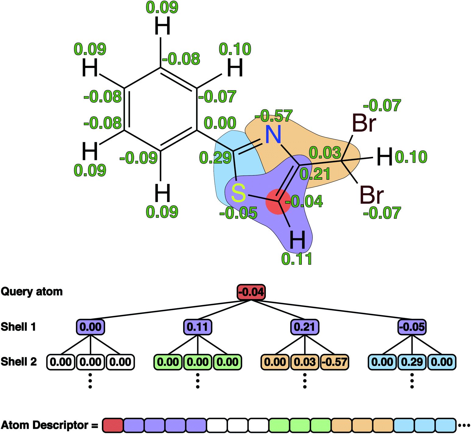Fig. 1 An illustration of the charge shell descriptor with values sorted according to the Cahn–Ingold–Prelog (CIP) rules. The green values correspond to the calculated CM5 charges using GFN1-xTB.

Dataset splitting

We utilize an unsupervised learning procedure similar to the one found in the MOLAN workflow by Sivaraman et al.,³⁰ which resembles the ButinaSplitter from DeepChem. The procedure is as follows: SMILES representations of each molecule are converted into extended connectivity (Morgan) fingerprints³¹ with radii of 2 and 1024 bits (ECFP4). The ECFP4 fingerprints are then used to construct a Tanimoto similarity matrix, which enables a clustering of the molecules using the Butina clustering algorithm³² with a radial cutoff of 0.6 as implemented in RDKit.²⁹ Clusters with at least 7 molecules are included in the training/test set and otherwise in the out-of-sample set to explore how well the trained machine learning models generalize. For some molecules either the descriptor or RegioSQM20 calculations fail, or the molecules are excluded due to Chauvenet's criterion, which left us with 21 201 reactions corresponding to 100 588 unique reaction sites. Thus, applying the above procedure results in a training/test set and an out-of-sample set of 15 246 and 5955 molecules, which correspond to 73 123 and 27 465 unique reaction sites, respectively.

Uniform stratified and random splits are then used to obtain a 80 : 20 ratio between the training and test sets resulting in 12 196 and 3050 molecules corresponding to 58 384 and 14 739 unique reaction sites, respectively. For the uniform stratified split, each of the individual clusters are randomly split and hereafter combined to ensure that both the training and test sets have similar representations of the underlying data distribution. On the other hand, the random split is indeed completely random with respect to all of the molecules obeying the cluster size cutoff.

As the strategy of this work is to learn and predict using atoms instead of molecules, all of the atomic descriptors for atoms in molecules belonging to the training, test, and out-of-sample sets are collected into different input sets and the corresponding proton affinities or classifications into different output sets.

An analysis of the training, test, and out-of-sample datasets can be found in the ESI.†

Machine learning models

In order to learn and predict the regioselectivity of EAS reactions, we explore various regression and classification models with respect to both the experimental and calculated data described above. Initially, a screening of 17 regression models and 13 classification models using PyCaret version 2.3.2 (ref. 33) is conducted (details can be found in the ESI†). This allows us to quickly find promising machine learning methods, which are then thoroughly examined in terms of finding optimal hyperparameters. The hyperparameter optimizations are carried out using a tree-structured Parzen estimator (TPE) as implemented in Optuna version 2.5.0.³⁴ All training and evaluation are done using either a normal or a stratified 5-fold cross-validation of the randomly shuffled training set in the case of the regression and classification models, respectively, and only the models with the best validation performance are saved for testing. As shown in Table S4† the best performance for both regression and classification is the ensemble decision tree variant called light gradient boosting machine (LightGBM) version 3.1.1 (ref. 35) using the sorted-shell atomic descriptors with a shell radius of 5. We refer to this method as simply “LightGBM” hereafter.

Furthermore, we examine the imbalance in the dataset using a “Null model”, where all sites are predicted to be non-reactive. And we employ a 1-nearest neighbor (1-NN) classifier as a baseline model using the brute-force search algorithm and the Jaccard (also known as Tanimoto) metric as implemented in scikit-learn,³⁶ which corresponds to a perfect memorization of the training set.³⁷

Results and discussion

The results we present here only involve the random splitting of the training/test set as similar performances are observed for both the stratified and random splits as seen in Table S5 in the ESI.† Unless otherwise noted, all machine learning models are classifiers that output a value between 0 and 1 for each atom, where a value greater than 0.5 indicates that an atom should be reactive.

Data-driven machine learning classifiers

In this section, we train and evaluate machine learning classifiers on experimental data collected from Reaxys consisting of 58 384, 14 739, and 27 465 unique reaction sites in the training, test, and out-of-sample sets, respectively. The experimental data often contain just single or a few reported reactive sites among all reaction sites in the reactant, i.e. there are significantly more negatives (N) than positives (P) in the dataset. Consequently the accuracy (the proportion of correct predictions, ACC) can be a misleading metric. For example, a “Null model”, where all sites are predicted to be non-reactive achieves a respectable accuracy of 76% (Table 1) for both the test and out-of-sample sets, but this just reflects the fact that 76% of the sites in both the datasets are unreactive. The Matthews correlation coefficient³⁸ (MCC) is a more robust metric to assess the model performance, since it also considers false positives (FP) and false negatives (FN) in addition to true positives (TP) and true negatives (TN).where are also known as precision, recall, specificity, and negative predictive value, respectively.

Table 1 Comparing different methods for predicting the reactivity of the 14 739 unique reaction sites in the test set and the 27 465 unique reaction sites in the out-of-sample set. The reported metrics are accuracy (ACC), Matthew's correlation coefficient (MCC), precision (PPV or positive predictive value), recall (TPR or true positive rate), specificity (TNR or true negative rate), and negative predictive value (NPV). All of the ML models are trained on the 58 384 unique reaction sites in the training set with two exceptions: the “RegioML (all reactions)” model is trained on all of the available data including the training, test and out-of-sample sets, and the “LightGBM (532 reactions)” model is trained on data from the RegioSQM20 paper⁶ in which 37 and 74 reactions are part of the test and out-of-sample sets, respectively. These reactions are therefore excluded from the reported statistics

Method	Test set						Out-of-sample set
	ACC	MCC	PPV	TPR	TNR	NPV	ACC	MCC	PPV	TPR	TNR	NPV
Null model	0.76	0.00	0.00	0.00	1.00	0.76	0.76	0.00	0.00	0.00	1.00	0.76
1-NN	0.86	0.62	0.71	0.72	0.91	0.91	0.81	0.49	0.59	0.64	0.86	0.88
RegioML	0.93	0.81	0.88	0.83	0.96	0.95	0.90	0.72	0.80	0.76	0.94	0.93
WLN (not retrained)	0.93	0.80	0.92	0.78	0.98	0.93	0.92	0.78	0.88	0.78	0.96	0.93
RegioML (all reactions)	0.99	0.98	0.99	0.99	1.00	1.00	0.99	0.98	0.99	0.98	1.00	0.99
RegioSQM20	0.89	0.70	0.75	0.81	0.91	0.94	0.88	0.69	0.73	0.80	0.91	0.94
LightGBM (532 reactions)	0.84	0.52	0.84	0.43	0.97	0.84	0.84	0.51	0.78	0.46	0.96	0.85
LightGBM RegioSQM20	0.88	0.69	0.75	0.78	0.92	0.93	0.86	0.62	0.69	0.74	0.89	0.92
RegioSQM20 PBEh-3c	0.90	0.73	0.81	0.78	0.94	0.93	0.90	0.72	0.79	0.79	0.93	0.93
LightGBM RegioSQM20
PBEh-3c	0.90	0.72	0.81	0.76	0.94	0.93	0.87	0.65	0.74	0.73	0.92	0.91
LightGBM RegioSQM20 regression	0.87	0.65	0.74	0.73	0.92	0.92	0.86	0.61	0.70	0.71	0.90	0.91

---

The MCC values for both the test and out-of-sample sets are zero, which clearly shows that the Null model lacks any real predictive power.

As a baseline model, we trained a 1-nearest neighbor (1-NN) classifier corresponding to a perfect memorization of the training set.³⁷ The data show that an impressive-looking 86% accuracy can be achieved for the test set by simple memorisation of the training set. In contrast, the MCC value is only 0.62 for the test set and considerably lower (0.49) for the out-of-sample set. These values primarily reflect a low precision where only 71% and 59% of the positive predictions are actually correct.

Our best machine learning model (LightGBM) achieves considerably better precisions of 88% and 80% for the test and out-of-sample sets, respectively. Note that while there is only a 3% drop in accuracy on going from the test set to the out-of-sample set, there is an 8% drop in the precision (and a concomitant drop in the MCC). Hereafter, we refer to this method (i.e. LightGBM trained on experimental data) as RegioML.

The test set MCC of RegioML is virtually identical to the Weisfeiler–Lehman neural network (WLN) architecture specifically trained to predict the regioselectivity of EAS reactions by Struble et al.⁸ While the precision is 4% higher for WLN, the recall (the fraction of positives that are predicted correctly) is 5% lower, leading to a nearly identical overall performance. WLN performs better on the out-of-sample set, with an MCC value that is nearly identical to that of the test set. However, it should be noted that many of the molecules in these two sets are likely included in the set used to train the WLN method, which is likely to inflate the MCC values of WLN. For example, we are able to achieve a MCC value of 0.98 on both the test and out-of-sample sets by training the LightGBM model on the entire collection of data using 10-fold cross-validation (the MCC value is for the best performing model).

Comparison to RegioSQM20

RegioSQM20 predicts the regioselectivity of EASs by finding the reaction center with the highest proton affinity. For computational efficiency, the proton affinities are computed using the semiempirical tight binding method GFN1-xTB and a continuum solvent model of MeOH. The centers with proton affinities within 1 kcal mol⁻¹ of the maximum are considered reactive. This method thus has only a handful of hyperparameters (choice of the computational method, solvent, energy cutoff, and conformational search method) and these are chosen based on a dataset of 532 experimental measurements, some of which are included in the current training set.

For the test set, the recall of RegioSQM20 is similar to that of RegioML (81% vs. 83%), but the precision is significantly worse (75% vs. 88%). For the out-of-sample set, the recall is somewhat better for RegioSQM20 (80% vs. 76%), but the precision is still worse (73% vs. 80%), leading to a slightly smaller MCC value of 0.69 compared to the 0.72 for RegioML. In contrast to RegioML, the overall performance of RegioSQM20 is very similar for the test and out-of-sample sets, as one would expect from a more physics based method. However, RegioSQM20 does not offer an advantage over RegioML for the out-of-sample dataset, while being computationally much more demanding (see below).

The main advantage of the RegioSQM20 approach is that it may offer an accuracy similar to that of RegioML based on a much smaller training set. Indeed a LightGBM model trained on the same 532 reactions used to develop RegioSQM20 results in MCC values around 0.5 for both the test and out-of-sample sets. While the precision is quite good for this model, the recall is less than 50% due to a large proportion of false negatives. Thus, in cases where little experimental data is available, physics-based methods such as RegioSQM20 are likely to outperform ML based methods, even if the latter rely on quantum descriptors such as atomic charges.

The computational expense of the physics-based methods can be mitigated by using them to generate synthetic data for the machine learning model. Indeed, a LightGBM classifier trained on RegioSQM20 predictions for the large training set of 58k reaction centers offers the same performance as that of RegioSQM20 for the test set. Of course, the performance is worse for the out-of-sample set just like for RegioML, but the training dataset can now easily be expanded to ensure a better coverage of chemical space. Furthermore, since RegioSQM20 is not used to offer real-time predictions to a user, more accurate and computationally expensive methods can be explored. For example, the precision of RegioSQM20 can be increased by 6% by using PBEh-3c single point calculations to compute the proton affinities – an increase that is reflected in the corresponding ML model. The overall performance of RegioSQM20 PBEh-3c is now identical to that of RegioML for the out-of-sample dataset, with a MCC value of 0.72.

We also explore whether it is better to predict proton affinities using regression and use them to identify reactive centers, rather than the classification approach. Although the LightGBM RegioSQM20 regression model is able to achieve a mean absolute error (MAE) of 2.00 kcal mol⁻¹ on the test set, its accuracy is not good enough to distinguish between reactive and non-reactive sites compared to that of the LightGBM RegioSQM20 model, as evidenced by the low recall values of 71–73%. However, the LightGBM RegioSQM20 regression model can be used to predict low, medium, or high reactivity as we showed in the RegioSQM20 paper.⁶ In fact, by combining the classification model and the regression model, one gets both regioselectivity predictions and a qualitative prediction of the reactivity of a molecule with almost no additional cost as the atomic descriptors only have to be calculated once. Examples of the output of RegioML can be seen in Fig. 2.

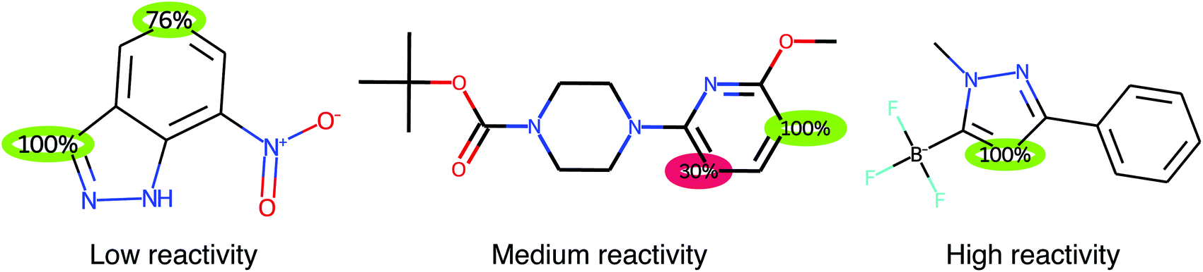Fig. 2 Examples of the output of RegioML. The scores are obtained by a LightGBM classification model, where values above 50% indicate that an atom should be reactive (green circles). However, atoms with scores above 5% are also highlighted (red circles). The predicted low, medium, or high reactivity is based on the highest proton affinity within the molecule obtained by a LightGBM regression model.

Timings

In Table 2 we compare the timings of the RegioSQM20 method, the RegioML model, and the WLN architecture by Struble et al.⁸ for the 3050 molecules in the test set. We report the median CPU time and the mean CPU time for predicting the regioselectivity of a molecule with a SMILES representation as input. For the RegioML model and the WLN architecture, the timings cover descriptor creation as well as model prediction for all reaction sites in the given reactant.

Table 2 Timings of the RegioSQM20 method, the RegioML model, and the WLN architecture for predicting the regioselectivity of the 3050 molecules in the test set with a SMILES representation as input. For the RegioML model and the WLN architecture, the timings include descriptor creation and model prediction for all reaction sites in the given reactant

Method	Median CPU time (s)	Mean CPU time (s)
a 4 Cores per molecule (Intel® Xeon® CPU E5-2643 v3 @ 3.40 GHz). b 1 Core per molecule (Intel® Xeon® CPU X5550 @ 2.67 GHz).
RegioSQM20^a	48	130
RegioML^b	0.46	0.69
WLN (not retrained)^b	0.03	0.03

---

The results show that the median CPU time requirements of the RegioSQM20 method is 48 s per molecule on four Intel® Xeon® CPU E5-2643 v3 @ 3.40 GHz cores. The RegioML model is almost 100 times faster on just a single Intel® Xeon® CPU X5550 @ 2.67 GHz core with a median CPU time of less than half a second per molecule. The WLN architecture is able to achieve a mean CPU time of just 0.03 s per molecule on the single Intel® Xeon® CPU X5550 @ 2.67 GHz core. The main reason for the slower performance of RegioML is the GFN1-xTB single point calculations needed to compute the atomic charges.

Conclusions and outlook

We present RegioML, an atom-based machine learning model for predicting the regioselectivities of electrophilic aromatic substitution (EAS) reactions. The model relies on ultra fast quantum chemical descriptor calculations combined with an ensemble decision tree variant called light gradient boosting machine (LightGBM). The atomic descriptors are based on CM5 atomic charges obtained from a single conformer embedded with RDKit²⁹ and single point calculations using the open source semiempirical tight binding method GFN1-xTB.²⁷ The model is trained and tested on 21 201 bromination EAS reactions corresponding to 101k reaction centers, which are split into a training, test, and out-of-sample datasets with 58k, 15k, and 27k reaction centers, respectively. The accuracy is 93% and 90% for the test and out-of-sample sets, respectively, but this is not a good measure of performance due to the preponderance of non-reactive sites. For example, the precision (the percentage of positive predictions that are correct) is 88% for the test set, but only 80% for the out-of-sample set. The final RegioML model released to users is trained on the entire data set and we expect similar performance for molecules in-sample and out-of-sample for this large dataset. For example, for a molecule in this large training set, we expect a precision of 99%, while for a molecule that is similar and out-of-sample, we expect a precision of 88% and 80%, respectively. The test-set performance is very similar to that of the graph-based WLN method developed by Struble et al.⁸ though the comparison is complicated by the possibility that some of the test and out-of-sample molecules are used to train WLN. RegioML out-performs our physics-based RegioSQM20 method⁶ where the precision is only 75%. Even for the out-of-sample dataset, RegioML slightly outperforms RegioSQM20.

The good performance of RegioML and WLN is in large part due to the large datasets available for this type of reaction. For example, if we retrain the RegioML model on the same 532 reactions we used to develop RegioSQM20, the performance is much worse due to a large increase in the false negative rate leading to a recall (the percentage of positives that are predicted correctly) below 50% compared to the 80% for RegioSQM20. Thus, one use of physics-based approaches such as RegioSQM20 is to generate synthetic data for the ML model for reactions where there is little experimental data. We demonstrate this by showing that the performance of RegioSQM20 can be reproduced by a ML model trained on RegioSQM20-generated data.

Data availability

RegioML is freely available under the MIT open source license at: https://github.com/jensengroup/RegioML.

Additional code for dataset curation and machine learning training is available at: https://sid.erda.dk/sharelink/HypB1igzDl.

Author contributions

AG and JHJ developed the idea and lead the project. NR wrote all the code and performed all the calculations. All authors contributed to the data analysis. All authors read and approved the final manuscript.

Funding

This work was supported by Bayer AG.

Conflicts of interest

The authors declare that there are no competing interests.

References

1. M. Hartenfeller, M. Eberle, P. Meier, C. Nieto-Oberhuber, K.-H. Altmann, G. Schneider, E. Jacoby and S. Renner, A collection of robust organic synthesis reactions for in silico molecule design, J. Chem. Inf. Model., 2011, 51, 3093–3098.
2. M. Liljenberg, T. Brinck, B. Herschend, T. Rein, S. Tomasi and M. Svensson, Predicting regioselectivity in nucleophilic aromatic substitution, J. Org. Chem., 2012, 77, 3262–3269.
3. K. Jorner, T. Brinck, P.-O. Norrby and D. Buttar, Machine learning meets mechanistic modelling for accurate prediction of experimental activation energies, Chem. Sci., 2021, 12, 1163–1175.
4. M. Kruszyk, M. Jessing, J. L. Kristensen and M. Jørgensen, Computational methods to predict the regioselectivity of electrophilic aromatic substitution reactions of heteroaromatic systems, J. Org. Chem., 2016, 81, 5128–5134.
5. J. C. Kromann, J. H. Jensen, M. Kruszyk, M. Jessing and M. Jørgensen, Fast and accurate prediction of the regioselectivity of electrophilic aromatic substitution reactions, Chem. Sci., 2018, 9, 660–665.
6. N. Ree, A. H. Göller and J. H. Jensen, RegioSQM20: improved prediction of the regioselectivity of electrophilic aromatic substitutions, J. Cheminf., 2021, 13, 10.
7. A. Tomberg, M. J. Johansson and P.-O. Norrby, A predictive tool for electrophilic aromatic substitutions using machine learning, J. Org. Chem., 2019, 84, 4695–4703.
8. T. J. Struble, C. W. Coley and K. F. Jensen, Multitask prediction of site selectivity in aromatic C–H functionalization reactions, React. Chem. Eng., 2020, 5, 896–902.
9. Y. Guan, C. W. Coley, H. Wu, D. Ranasinghe, E. Heid, T. J. Struble, L. Pattanaik, W. H. Green and K. F. Jensen, Regio-selectivity prediction with a machine-learned reaction representation and on-the-fly quantum mechanical descriptors, Chem. Sci., 2021, 12, 2198–2208.
10. W. Beker, E. P. Gajewska, T. Badowski and B. A. Grzybowski, Prediction of major regio-, site-, and diastereoisomers in Diels–Alder reactions by using machine-learning: The importance of physically meaningful descriptors, Angew. Chem., Int. Ed. Engl., 2019, 58, 4515–4519.
11. M. Moskal, W. Beker, S. Szymkuć and B. A. Grzybowski, Scaffold-Directed Face Selectivity Machine-Learned from Vectors of Non-covalent Interactions, Angew. Chem., Int. Ed., 2021, 60, 15230–15235.
12. L. Wang, C. Zhang, R. Bai, J. Li and H. Duan, Heck reaction prediction using a transformer model based on a transfer learning strategy, Chem. Commun., 2020, 56, 9368–9371.
13. X. Li, S. Zhang, L. Xu and X. Hong, Predicting regioselectivity in radical C–H functionalization of heterocycles through machine learning, Angew. Chem., Int. Ed., 2020, 59, 13253–13259.
14. R. Roszak, W. Beker, K. Molga and B. A. Grzybowski, Rapid and accurate prediction of pK_a values of C–H acids using graph convolutional neural networks, J. Am. Chem. Soc., 2019, 141, 17142–17149.
15. S. Grimme, J. G. Brandenburg, C. Bannwarth and A. Hansen, Consistent structures and interactions by density functional theory with small atomic orbital basis sets, J. Chem. Phys., 2015, 143, 054107.
16. M. Cossi and V. Barone, Analytical second derivatives of the free energy in solution by polarizable continuum models, J. Chem. Phys., 1998, 109, 6246–6254.
17. M. Garcia-Ratés and F. Neese, Efficient implementation of the analytical second derivatives of Hartree–Fock and hybrid DFT energies within the framework of the conductor-like polarizable continuum model, J. Comput. Chem., 2019, 40, 1816–1828.
18. F. Neese, Software update: The ORCA program system, version 4.0, Wiley Interdiscip. Rev.: Comput. Mol. Sci., 2018, 8, e1327.
19. M. Rupp, A. Tkatchenko, K.-R. Müller and O. A. von Lilienfeld, Fast and accurate modeling of molecular atomization energies with machine learning, Phys. Rev. Lett., 2012, 108, 058301.
20. A. R. Finkelmann, A. H. Göller and G. Schneider, Robust molecular representations for modelling and design derived from atomic partial charges, Chem. Commun., 2016, 52, 681–684.
21. A. R. Finkelmann, A. H. Göller and G. Schneider, Site of metabolism prediction based on ab initio derived atom representations, ChemMedChem, 2017, 12, 606–612.
22. A. R. Finkelmann, D. Goldmann, G. Schneider and A. H. Göller, MetScore: Site of metabolism prediction beyond cytochrome P450 enzymes, ChemMedChem, 2018, 13, 2281–2289.
23. C. A. Bauer, G. Schneider and A. H. Göller, Gaussian process regression models for the prediction of hydrogen bond acceptor strengths, Mol. Inf., 2018, 38, 1800115.
24. C. A. Bauer, G. Schneider and A. H. Göller, Machine learning models for hydrogen bond donor and acceptor strengths using large and diverse training data generated by first-principles interaction free energies, J. Cheminf., 2019, 11, 59.
25. L. Kuhnke, A. ter Laak and A. H. Göller, Mechanistic reactivity descriptors for the prediction of Ames mutagenicity of primary aromatic amines, J. Chem. Inf. Model., 2019, 59, 668–672.
26. A. V. Marenich, S. V. Jerome, C. J. Cramer and D. G. Truhlar, Charge model 5: An extension of Hirshfeld population analysis for the accurate description of molecular interactions in gaseous and condensed phases, J. Chem. Theory Comput., 2012, 8, 527–541.
27. S. Grimme, C. Bannwarth and P. Shushkov, A robust and accurate tight-binding quantum chemical method for structures, vibrational frequencies, and noncovalent interactions of large molecular systems parametrized for all spd-block elements (Z = 1–86), J. Chem. Theory Comput., 2017, 13, 1989–2009.
28. S. Wang, J. Witek, G. A. Landrum and S. Riniker, Improving conformer generation for small rings and macrocycles based on distance geometry and experimental torsional-angle preferences, J. Chem. Inf. Model., 2020, 60, 2044–2058.
29. RDKit, Open-Source Cheminformatics (version 2020.09.4), http://www.rdkit.org.
30. G. Sivaraman, N. E. Jackson, B. Sanchez-Lengeling, Á. Vázquez-Mayagoitia, A. Aspuru-Guzik, V. Vishwanath and J. J. de Pablo, A machine learning workflow for molecular analysis: Application to melting points, Mach. Learn.: Sci. Technol., 2020, 1, 025015.
31. D. Rogers and M. Hahn, Extended-connectivity fingerprints, J. Chem. Inf. Model., 2010, 50, 742–754.
32. D. Butina, Unsupervised data base clustering based on Daylight's fingerprint and Tanimoto similarity: A fast and automated way to cluster small and large data sets, J. Chem. Inf. Comput. Sci., 1999, 39, 747–750.
33. M. Ali, Pycaret: An Open Source, Low-Code Machine Learning Library in Python, PyCaret version 2.3.2, 2020.
34. T. Akiba, S. Sano, T. Yanase, T. Ohta and M. Koyama, Optuna: A next-generation hyperparameter optimization framework, Proceedings of the 25th ACM SIGKDD International Conference on Knowledge Discovery and Data Mining, 2019.
35. G. Ke, Q. Meng, T. Finley, T. Wang, W. Chen, W. Ma, Q. Ye and T.-Y. Liu, LightGBM: A highly efficient gradient boosting decision tree, Proceedings of the 31st International Conference on Neural Information Processing Systems, Red Hook, NY, USA, 2017, pp. 3149–3157.
36. F. Pedregosa, et al., Scikit-learn: Machine learning in Python, J. Mach. Learn. Res., 2011, 12, 2825–2830.
37. I. Wallach and A. Heifets, Most ligand-based classification benchmarks reward memorization rather than generalization, J. Chem. Inf. Model., 2018, 58, 916–932.
38. B. Matthews, Comparison of the predicted and observed secondary structure of T4 phage lysozyme, Biochim. Biophys. Acta, Protein Struct., 1975, 405, 442–451.

---

Footnote

† Electronic supplementary information (ESI) available. See DOI: 10.1039/d1dd00032b

---