Machine learning platform for determining experimental lipid phase behaviour from small angle X-ray scattering patterns by pre-training on synthetic data

Abstract

Lipid membranes are vital in a wide range of biological and biotechnical systems; they undepin functions from modulation of protein activity to drug uptake and delivery. Understanding the structure, interactions, self-assembly and phase behaviour of lipids is critical to developing a molecular undertanding of biological membrane mediated processes, establishing engineering approaches to biotechnical membrane application development. Small Angle X-ray Scattering (SAXS) is the de facto method used to analyse the structure of self-assembled lipid systems. The resultant diffraction patterns are however extremely difficult to assign automatically with researchers spending considerable time often analysing patterns ex situ from a beamline facility, reducing experimental capacity and optimisation. Furthermore, research projects will often focus on particular lipid compositions and thus would benefit significantly from a method which can be rapidly optimised for a range of samples of interest. We present a generalisable machine learning pipeline that is able to classify lipid phases based on their raw, experimental SAXS spectra, with >99% accuracy and an inference time of <60 ms, enabling high throughput on-site analysis. We achieved this through application of a synthetic data generation system, capable of building synthetic SAXS patterns from the underlying physics which dictate phase behaviour, and we also propose an extension of our system to synthetically generate co-existence phase spectra with known composition ratios. Pre-training our machine learning model on this synthetic data, and fine-tuning on experimental samples empowers the model in achieving state-of-the-art, rapid lipid phase classification, allowing researchers to be able to adapt their experiments on site if needed and hence massively accelerate high throughput lipid research.

---

Introduction

Lipid molecules can self-assemble into a huge variety of different liquid crystalline phases.¹ These phases can exist as either lamellar phases, where lipids form a bilayer structure,² or as more complex non-lamellar structures, such as inverse hexagonal (H_II)³ and inverse bi-continuous cubic phases (Q_II).⁴ Lipid phases are readily and controllably interconvertible through altering parameters which can include chemical composition,⁵ temperature,⁶ pressure, and pH.⁷ This enables cells to modulate protein activity,⁸ impact signalling pathways⁹ and to facilitate membrane fusion events.¹⁰ Furthermore, within biotechnological fields, the ability to controllably form a variety of lipid phases has been exploited to template hydrogels¹¹ and nanowires,¹² produce cargo delivery systems¹³ and protein crystallisation complexes.¹⁴ As both in vivo and in vitro uses of polymorphic lipid behaviour rely on the generation of particular lipid phases, identification of the membranes structural character is pivotal.

A method that is commonly employed to study lipid phase behaviour is small angle X-ray scattering (SAXS).^15,16 SAXS enables lipid structures to be assigned through the detection and indexing of Bragg X-ray diffraction peaks. The relative position of the Bragg peaks in the diffraction pattern enables the identification of a lipid phase through characteristic Bragg peak position ratios.¹⁷ Detailed analysis of the diffraction patterns allows the extraction of the structural information of lamellar,^18–20 cubic^21–24 and hexagonal^3,25,26 phases at the molecular scale. Through the use of high brightness synchrotron light sources, the kinetics of rapid phase transitions can be probed,²⁷ where increased understanding of lipid phase behaviour has led to the handling of increasingly complex structures.²⁸ Increasing light source brightness and detector frame rates offers the possibility of probing membrane structural transitions with ever greater time resolution and detail, but this increase in data presents significant analysis challenges.²⁹ A current typical synchrotron SAXS experimental workflow requires the researcher designing experiments to formulate mixtures either prior to the experimental time or at a laboratory at the beamline facility followed by performing the SAXS experiments. Analysis of scattering patterns is a time consuming and intensive process. Current lipid SAXS data analysis bottlenecks often necessitate off-line data analysis after an experiment has been completed. During high throughput synchrotron SAXS experiments, near real-time analysis offers the opportunity of optimising experimental planning and scientific output. Synchrotron beamtime is often limited and follow up experiments may be difficult to conduct in a timely manner. This effect is magnified by the ever-increasing volume of data to be analysed – as beamline techniques have matured³⁰ and the rate of data acquisition has followed accordingly. Additionally, in many cases, there may be a range of interpretations of the structure and dynamics of these phases. With human analysis, this can introduce classification bias, which can be significant in complex SAXS patterns, such as those that demonstrate phase coexistence in which individual patterns may exist together simultaneously. Several software tools such as AXcess,³¹ DPDAK,³² or DAWN³³ have been developed to assist in the processing of large amounts of data, including 2D diffraction images. In addition, basic analysis such as peak finding and fitting may also be performed with these programmes. However, these tools are not optimized to identify lipid phases and/or to deal with samples exhibiting multiple coexisting phases. This need has been partially addressed in software suites such as scatter³⁴ or SCryPTA,³⁵ which help the user to identify the lipid mesophase by displaying the peak positions for a given phase and first peak, yet this requires manual validation preventing high throughput analysis of the SAXS data. Other tools, such as those described by Joseph et al.³⁶ or Dully et al.³⁷ compare the ratios between peak positions with respect to those of known lipid polymorphs, allowing to extract the lipid mesophase without the need of user input. However, such approaches have limited success when dealing with coexisting lipid phases. To the best of our knowledge, there exists no method to automatically, quantitatively assign the degree of coexistence within a sample.

Machine learning (ML) based data analysis techniques have recently boomed due to the improved accessibility and unprecedented performance they offer across many different tasks,^38,39 from sentiment analysis to image classification and object detection.⁴⁰ The task-agnostic nature of these algorithms allow specific pipelines to be developed to allow predictability of a certain task. ML algorithms often require large datasets to achieve their maximum potential predictability,⁴¹ this aligns well with the high throughput nature of beamlines.³⁰ Recently, ML tools have been used for studying bio-macromolecular solutions of diverse protein structural units,⁴² predicting the physical properties of ionic liquids,⁴³ estimating the structure of ternary lipid phase diagrams,⁴⁴ and to study gel to fluid lipid bilayer transitions.⁴⁵ Additionally, recent previous works show that ML has the potential to predict lipid phase behaviour within a small experimental sample space, with reports of 66–96% accuracies depending on the specific phase being predicted.^46–48 However, no prior robust systems for generalised lipid phase analysis across multiple phases which achieve >99% accuracy have been developed.

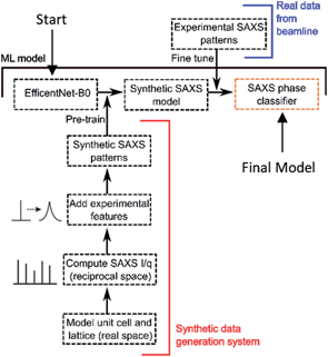
In this study, we demonstrate that a convolutional neural network (CNN),⁴⁹ pre-trained on synthetic SAXS data and fine-tuned on real SAXS patterns, allows for the successful identification of real and synthetic SAXS patterns without human intervention at runtime. To satisfy a sparsity in experimental data, a synthetic data generation system was built through meshed electron density models in real space and then transformed to Fourier space. Through this bespoke CNN we have unlocked phase predictions for a multitude of potential structures, including lamellar, hexagonal, and cubic gyroid, diamond, and primitive phases on real, unlabelled, experimental SAXS data as well as synthetically generated SAXS patterns. We have made our model public access (https://github.com/GouldGroup/SAXSpy) in the hope that the lipid SAXS community can find application for and engage with the model in a multitude of analytical settings.

Method

Unsupervised learning techniques were first used both as tools for exploratory data analysis, as well as to attempt to classify and label our experimental SAXS samples. The performance of unsupervised learning on our phase classification task was limited (see results). As such, our supervised learning pipeline was developed to allow lipid phase prediction for labelled experimental SAXS patterns (Fig. 1).

Fig. 1 Flow diagram of our ML pipeline. We start with an initial EfficientNet model convolutional neural network (CNN), global average pooling and a classification head to map the abstracted features to the 6 classifications (phases – blank, lamellar, hexagonal, P cubic, G cubic, D cubic). The model is pre-trained on synthetically generated SAXS patterns to make our SAXS model classifier. This is then fine-tuned on real, experimental SAXS patterns to form our final SAXS phase classifier model.

Synthetic data modelling

Model SAXS patterns were generated by building meshed electron density models of each phase to represent the lamellar (L, in 1D), hexagonal (H_II, in 2D) and cubic phases (Q_II, in 3D). The modelling details of the unit cell and lattice for each phase are provided in the ESI.† For each phase, the SAXS intensity is given by:

I(q) = |F(q)|²S(q)

where I(q) is the peak intensity at a given wavenumber, F(q) is the form factor (the Fourier transform of the electron density function) of a single unit cell, and S(q) is the reciprocal lattice. Once the initial peak positions and intensity values (I/q) were computed, additional features were added to simulate experimentally observed SAXS patterns. These included introducing Voigt signals at the peaks to model the imperfect peak widths found in real spectra and a Debye–Waller dampening factor,^46,50 to simulate exponential signal decay at larger wavenumbers, due to thermal fluctuations of the interfaces. Further non-peak specific features were also added such as a broad polycarbonate scattering peak which simulates the scattering usually observed from sample capillaries in experimental SAXS patterns.

For each phase, the model parameters were optimised to minimise the variance between the synthetic samples and the real, experimentally obtained patterns. The parameter range was then expanded about the central parameters such that a larger phase space was generated for model training (see ESI† for full parameter list).

The synthetic data generation package was written using Python 3.8, with mathematical operations and linear algebra performed using the NumPy⁵¹ 1.19.2 and SciPy⁵² 1.3.1 packages. Data featurization and pre-processing was also performing with the NumPy package. Tenserflow⁵³ 2.6.0 was used to implement our model and training procedure. The model was trained using a GTX 1080 Ti graphical processing unit (GPU) for ∼5 min per epoch for pre-training and ∼50 s per fine-tuning epoch.

Results and discussion

Lamellar phase modelling

The lamellar phase Bravais lattice can be modelled in one dimension, this gives a reciprocal lattice with lattice parameter a.

Modelling the electron density as three overlapping Gaussians that represent the bilayer head group and terminal methyl group positions gives a form factor of:

where L is the bilayer diameter, σ₁ is the electron density of the headgroup and σ₂ is the electron density of the terminal methyl group.

Inverse hexagonal phase modelling

The inverse hexagonal phase is composed of inverse micellar lipid cylinders that are packed hexagonally perpendicular to the z-coordinate. This symmetry enables the inverse hexagonal phase to be modelled in two dimensions. By taking a set of reciprocal lattice points along the radius from the origin a one-dimensional set of scattering points in reciprocal space is obtained.

The form factor for the inverse hexagonal phase was modelled using a polar coordinate system, akin to lamellar with two Gaussians for the lipid head and tail. In reciprocal space, this gives a form factor of:

where ρ(r) is the electron density, which is univariate due to the radial symmetry observed within the hexagonal phase, J₀ is the zeroth-order Bessel function and r is the radial position in the lattice.⁵⁴

Inverse Bi-continuous cubic phase modelling

To model the cubic phase, we based our model on a modification of the model presented by Garstecki and HoŁyst.^21–23 Like Garstecki and HoŁyst's model, our Triply Periodic Minimal Surface (TPMS) was generated using trigonometric approximations, but rather than using a rectangular bilayer function in three dimensions, our TPMS was decorated with two Gaussian convolved Kronecker delta functions to give the form factor:
where the triangulated TPMS is vectorised in 3D such that r_j is the position of the of the jth triangle centre, n_j is the normal unit vector to the triangle centre, L is the hydrocarbon width within the lipid bilayer, s_j is the surface area of the surface triangle and σ is the width of the Gaussian. Since r is the vector position of the triangle centre, which is sampled along the reciprocal lattice. The intensity value can thus be computed as a function of the wavevector:

The wave vector q is defined here with the Miller indices along the surface

Data exploration

Due to the availability of real data, lamellar and hexagonal phases were labelled and explored for evaluating the performance of unsupervised algorithms. SAXS patterns were first analysed through dimensionality reduction techniques, such that all the patterns (synthetic and real) could be visualised together, and their clustering explored. The patterns were mapped onto two-dimensional vector space. Dimensionality reduction followed by clustering is an example of unsupervised leaning, where the features of the data alone can be used to effectively label, or separate data based on the features within it. Compared to supervised techniques, unsupervised approaches typically incur reduced data requirements and are less time consuming. We utilised principal component analysis (PCA),^55,56 t-distributed stochastic neighbour embedding (t-SNE)⁵⁷ and uniform manifold approximation and projection (UMAP)⁵⁸ to explore our datasets. These dimensionality reduction techniques allow the visualisation of multiple features within a large dataset on a 2D latent space. PCA is a linear model which changes the basis of the high dimensional data by maximising the variance.

t-SNE and UMAP tend to perform better on non-linear data.^57,58 We therefore use all three techniques to be able to observe a representative view of the high dimensional SAXS data.

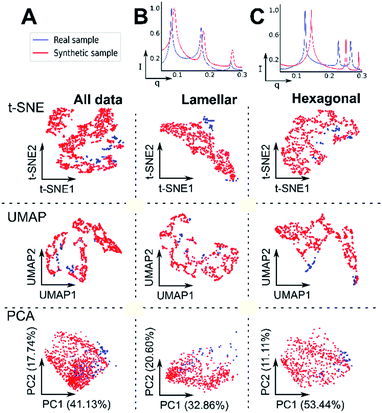
We first sought to answer whether our synthetic data generation system produced patterns that are representative of real, experimentally obtained SAXS patterns. This was important as our synthetic data, when visually compared to real data, appeared indistinguishable. In 2D space, a single, indistinguishable cluster was observed for both real and synthetic data with PCA. A single cluster was present when the data was considered as a combined multi-phase dataset (lamellar and hexagonal from each set – Fig. 2A) and when considered as a single-phase dataset (pure lamellar, Fig. 2B and pure hexagonal phases from each set, Fig. 2C). For PCA, over half of the measured variance was captured in the first two components for each model pair (e.g.Fig. 2A – variance PC1 + PC2 = 58.87%). Interestingly, t-SNE indicated a somewhat reasonable separation for real and synthetic lamellar but not for hexagonal patterns, with UMAP showing a similar separation for hexagonal, but not lamellar patterns. In t-SNE and UMAP, real data shows close proximity to synthetic in both lamellar and hexagonal datasets.

Fig. 2 Dimensionality reduction techniques indicate substantial overlap of real and synthetic datasets results depicting PCA, t-SNE and UMAP algorithms as applied to labelled real and synthetic datasets used for model training. In all instances the algorithms reduced the dimensionality to 2D vector space. The data was centred and transformed before projection. From the total synthetic dataset, 500 synthetic samples were randomly selected and 40 real samples are overlain, as indicated by colours. Results show comparing all data ((A) – 1000 synthetic and 80 real), the lamellar dataset ((B) – 500 synthetic and 40 real) and the hexagonal dataset ((C) – 500 synthetic and 40 real). Pattern intensity values were selected from q = 0.01–0.43, in each PCA instance, agreeable variance was retained. Pattern inserts at top show examples of I/q plots for synthetic and real data prior to dimensionality reduction.

A cluster in Fig. 2A t-SNE was observed in the top left of the plot and in the top right for UMAP; this suggests that our synthetic data covers a much larger range of possible parameters for each phase whilst constraining the significant features of each phase. The dimensionality reduction plots qualitatively show that real samples of the same phase, are not seen in the same cluster, whereas with synthetic samples, they tend to remain confined within a well-defined structure, which suggests that our synthetic parameters are more consistent.

Using the same techniques, we next sought to ask whether we could determine a means to separate phase patterns alone, without the need for a supervised approach. We compared lamellar and hexagonal patterns in both the synthetic and real datasets.

For real samples, two clusters were observed with UMAP and PCA although significant overlap of sample labelling was observed in each cluster, suggesting that the phases were inseparable based on their variances, this may be due to large peak overlap between the phases (Fig. 3A). Interestingly t-SNE indicated a single cluster with apparent label separation although overlap of lamellar was observed with hexagonal. t-SNE was also run following dimensionality reduction with a 10 component PCA and a near identical distribution was observed (ESI† and Fig. 3). For synthetic data (Fig. 3B), t-SNE and UMAP, lamellar and hexagonal show clear clustering with no significant clustering observed with PCA. It is known that t-SNE and UMAP cluster distance carries minimal meaningful information regarding the high dimensional data distance and density and thus were only used for data visualisation. For PCA however, we used K-means clustering⁵⁹ with 2 clusters in 4D and 10D (accounting for 72.9% and 89.9% of the total variance respectively) to attempt to separate our real lamellar and hexagonal phase patterns, this achieved a maximum accuracy of 75% at 4D with no increase in accuracy going to 10D. In tandem the dimensionality reduction⁶⁰ results show that a uniform unsupervised method is unable to significantly label real data and as such a supervised approach was developed.

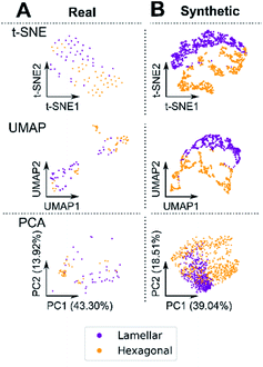Fig. 3 Unsupervised separation of lamellar and hexagonal phases using data visualisation and clustering. Data was sampled as in Fig. 2. Real hexagonal and lamellar data cannot be separated by clustering, whilst synthetic can, albeit with overall variance-preserving, non-linear algorithms, and some label overlap. Since these algorithms do not preserve high-dimensional distance/density information – neither synthetic nor real SAXS pattern phases can be separated using unsupervised clustering/dimensionality reduction techniques.

Model and data featurization

Our main objective was to optimise the model performance to inference time ratio; a supervised learning approach with the synthetically generated SAXS data was used to maximise model performance. A Cubic spline interpolation was used to maintain a fixed input shape for the model as well as a constant data point interval for each SAXS pattern.

Data

For each of the non-cubic lipid phases, 10 000 SAXS patterns were synthetically generated for training, with 6040 patterns for each of the cubic phases (Table 1). The data was generated based on the theoretical model and parameterisation shown prior. Stratified sampling was used such that the relative proportions of each phase in the dataset were representative of the likelihood of encountering such a phase – based on our real-patterns dataset. For the “Blank” phase category, only real blank samples were used and augmented by adding noise to each sample's signal.

Table 1 Overview of the datasets used in this work and the proportions of each phase, all data in the fine-tune, valid and test sets are real, experimentally obtained SAXS patterns except for cubic phases which are synthetically generated

Dataset	Phase
	Blank	Lamellar	Hexagonal	P Cubic	G Cubic	D Cubic
Pre-train	10 000	10 000	10 000	6040	6040	6040
Fine-tune	40	40	40	40	40	40
Valid	10	10	16	40	40	40
Test	10	20	17	7	7	7
Synth test	10 000	10 000	10 000	5000	5000	5000

---

In general, the model's input data and hence performance, relies heavily on the number of samples for each phase contributed by researchers. Since cubic lipid phases are rare, the synthetic data empowers the model to allow it to predict even the rare occurrences of cubic phase patterns. It is important to note, however, that all the cubic data used for training and validation were synthetically generated.

Data featurization

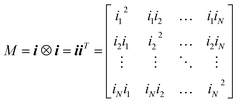
For each SAXS feature vector i of N datapoints from the pre-processed SAXS pattern, the outer product of the vector with its transpose was taken, such that a 2D matrix M of intensity values I and q valued indices was generated for each pattern.

i = (i₁, i₂, …, i_N)

where N = 200. This representation of the SAXS patterns allows for greater flexibility for neural modelling. The increased multi-dimensional spatial separation and value scaling allows a convolution kernel to more effectively abstract nuanced information from the SAXS pattern whilst the constant q value matrix indices are used as embedded positional encodings which provide an additional enforcement of spatial information.⁴⁹

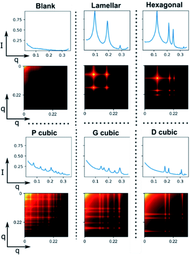
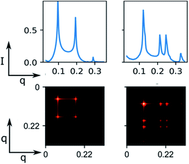
This representation also makes it easier to visualize peak pattern relationships at-a-glance (Fig. 4), since peaks are shown as points of high intensity, shoulder peaks and peak breadth are shown as an aura around the centre peak and the pattern remains consistent for each phase with the only variance being limited to the position of the pattern within the matrix and the intensity value. This depiction of the phase highlights the characteristic Bragg peak ratio in 2D space.

Fig. 4 2D feature map representation of sample SAXS patterns from our synthetic dataset. Each feature map is a result of the outer product of the intensity values vector with itself for each SAXS pattern shown above the map. Since the q range and intervals are fixed, the map indices can be used to determine the q values, with the matrix values being the intensity product.

It can also be seen that whilst lamellar and hexagonal have sharp and well-defined points of intensity, the cubic phases are more blurred. This is mainly due to the low intensity nature of cubic phases. However, a visual distinction is still maintained between all phases in the 2D feature maps.

As suggested with unsupervised learning, Fig. 4 and 5 in conjunction illustrate how the feature map is universally consistent across both synthetic and real samples. Furthermore, a clear distribution is observed for each phase, even with normally ambiguous SAXS patterns (see ESI†). It would appear that this consistency, with the added spatial separation, allows our ML model to perform significantly more robustly than using the standard I/q patterns, or even the pre-integrated beamline ring image – where the distinct phase information is more sparsely distributed.

Fig. 5 2D map representation of sample SAXS patterns from our real-samples dataset, the top row is the initial, interpolated SAXS pattern, with the bottom row being the 2D feature map representation of that pattern. The left column is an example of a lamellar phase sample with the right being hexagonal. A more crystalline lamellar sample is shown here to note distinction in the 2D space.

From this technique, we also propose a potential extension for this method from the assumption of phase co-existence as a linear combination of the SAXS pattern for each of the respective phases. A 2D feature map may enable a model to effectively scan various features across different lipid phases (Fig. 6). The feature map can be decomposed by the neural network into its separate phases, introducing information to the classification head regarding the composition of the co-existence sample.

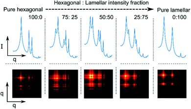Fig. 6 Synthetic phase co-existence feature map based on weighted, synthetic pure hexagonal and lamellar phase.

Although intensity magnitudes vary between each phase and its co-existing phase, each signals' peaks remain distinguishable by our model. Co-existing synthetic data may be generated using this method by taking a weighted sum of the outer product between two pure synthetic phases.

The label for co-existence can thus be defined as the proportion of each of pure samples, enabling some degree of mapping between the probability distribution of the model's predictions and the phase proportions, whilst simultaneously penalising overconfident models.

Model

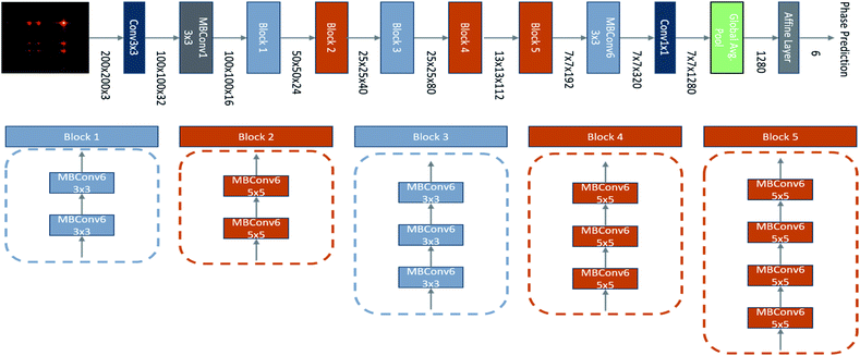
In order to satisfy our criteria of maximising accuracy whilst minimising inference time and computation to allow real-time analysis, we used the EfficientNet-B0 model architecture⁶¹ as our basis (Fig. 7). This model is the smallest and hence fastest of the EfficientNet family.⁶¹ Its architecture was determined using a Neural Architecture Search (NAS)^62,63 and it exploits mobile inverted bottleneck convolutions (MBConv)⁶⁴ to maximise accuracy at minimal computational requirements. Our model limits the input feature map resolution to 200 × 200, this limits memory usage without compromising on accuracy, further increases in map resolution yielded similar accuracy. A single feed-forward layer was used as the classification head with a softmax activation function, this proved sufficient as making the classification head deeper yielded the same, or worse accuracies. Global Average Pooling (GAP)⁶⁵ was performed on the features extracted by the CNN to reduce its dimensionality whilst minimising overfitting and the number of optimisable network parameters prior to the classification head. Not only is GAP more efficient than further fully connected layers, but it is more robust to spatial transformations since the spatial abstractions extracted by the CNN are compressed in a way that is more intuitive following spatial convolutions.

Fig. 7 Model architecture of our SAXS phase classifier. Each convolution block can be broken up into a set of MBConv operations with varying kernel properties and dimensions. The deeper we traverse through the network (from left to right) the more the spatial dimensions are reduced, and the number of convolution kernels is increased. The architecture is relatively shallow with each convolution being a depth wise separable convolution to minimise computational cost.

Training-procedure

The network weights were initialised based on the noisy-student EfficientNet-B0 pre-trained weights.⁶⁶ After broadcasting the feature map across the three channels, they were passed through the network with a dropout of 0.1 on the classification nodes during training.

The objective function used was categorical cross-entropy loss

The loss was computed after every batch with batch size = 8 and normalized accordingly. The use of MBConv layers and swish activations within the CNN prevented vanishing and exploding gradient problems, no gradient clipping or artificial gradient techniques were needed. The samples were fed into the model in two stages, pre-training and fine-tuning (Table 1). During the pre-training stage the model was trained on only synthetic data for two epochs, during which the loss was decreasing and the rate of decrease of the loss was also decreasing as expected (see ESI† for loss curves). The loss during the second epoch began fluctuating, suggesting further training epochs would result in overfitting. For each training stage, the adaptive gradient optimiser, Adam⁶⁷ was used with a learning rate of 0.01. A learning rate decay scheme was used such that for each epoch, the learning rate was conditionally scaled by a factor of 0.1 per epoch if the loss had plateaued.

In the fine-tuning stage, real, experimentally obtained SAXS patterns, from the fine-tune dataset were fed through the model (Fig. 1 and Table 1). The model was trained for up to 20 epochs on this set, with the same learning rate decay scheme applied, with patience of 10 epochs. The performance of the model in correctly identifying phases is shown to be strong, with values attaining 99.6% accuracy with our training procedure.

Tables 2 and 3 show that longer pre-training on synthetically generated SAXS patterns significantly improves our model's predictions. Further pre-training on synthetic data does improve the synthetic validation accuracy however, the test accuracy is reduced, suggesting overfitting. For each of the 5 epochs, both the validation and test accuracies fluctuate, with the test accuracy having an upwards general trend, these fluctuations can thus be attributed to the stochastic nature of the Adam optimiser. The fluctuation in the synthetic accuracy suggests that the optimisation landscape across both sets is not smooth, with the synthetic minima being much broader.

Table 2 Model accuracies for predicting the lipid phase behaviour based on a SAXS pattern from both our synthetic and real datasets after pre-training on synthetic SAXS patterns for 1 epoch. Longer pre-training significantly improves model accuracies (Δ + 3%). Whilst fine-tuning for more epochs also significantly improves accuracy then plateaus at different stages based on the amount of pre-training. Accuracy values shown as percentages

Fine-tune epochs	Valid/test accuracy (%)	Synthetic test accuracy (%)
0	54.9	98.3
5	95.5	97.7
10	92.4	94.8
15	96.9	98.8
20	96.9	96.3

---

Table 3 Model accuracies for predicting the lipid phase behaviour based on a SAXS pattern from both our synthetic and real datasets after pre-training on synthetic SAXS patterns for 2 epochs. Longer pre-training significantly improves model accuracies (Δ + 3%). Whilst fine-tuning for more epochs also significantly improves accuracy then plateaus at different stages based on the amount of pre-training. Accuracy values shown as percentages

Fine-tune epochs	Valid/test accuracy (%)	Synthetic test accuracy (%)
0	62.5	99.6
5	96.9	97.8
10	98.2	98.0
15	92.4	99.2
20	99.6	99.5

---

There is also a general upwards trend with increasing the number of fine-tune epochs on the accuracy, however this plateaus at around 10 epochs (Fig. 8), with further fine-tuning introducing marginal fluctuations in the model's accuracy, this suggests that further fine-tuning may result in overfitting and that larger fine-tune datasets may improve model performance.

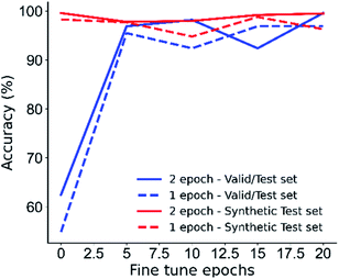Fig. 8 Model accuracy with fine-tuning epochs, more fine-tuning results in better model performance until approximately 10 epochs where accuracy begins to fluctuate.

Conclusions

Assigning the lipid phase observed from a SAXS pattern has been the limiting factor in many lipid researchers' workflows. We have shown that SAXS patterns can be theoretically modelled and that our synthetically generated data is valid. This data improved the performance of our phase prediction model, satisfying the requirement of large, varied datasets to train a robust deep learning model. We have successfully developed a complete ML pipeline that is state-of-the-art in predicting lipid phase behaviour with 99.6% accuracy on experimentally obtained SAXS data, with an inference time faster than humans on a home computer or mobile CPU. Our model is fine-tuned on real SAXS data, with no arbitrary rules on lipid phase behaviour. We hope that with this model, lipid researchers can quickly experiment with their samples at the beamline to generate more meaningful data, at high throughput and to enable researchers to quickly adapt their experiments based on their initial results. We have released the full pipeline code (https://github.com/GouldGroup/SAXSpy), from synthetic SAXS data generation to model training. Researchers can rapidly train their own SAXS prediction model to suit their needs using the optimal model. We hope that this work contributes to lipid research data analysis becoming more accessible and transparent.

Data availability

We have released the full pipeline code (https://github.com/GouldGroup/SAXSpy), from synthetic SAXS data generation to model training. This includes all experimental data which was used in the training of the model.

Conflicts of interest

There are no conflicts to declare.

Acknowledgements

HAA is supported by an awarded doctoral training studentship of the Engineering and Physical Sciences Research Council (EPSRC – EP/R513052/1) with training from the Institute of Chemical Biology (Imperial College London). The authors would like to thank Dr Chi L. Chan for their useful discussions and suggestions regarding the experimental data. We acknowledge Diamond Light Source for time on Beamline I22 under Proposals SM20789 and SM24537, and we would like to thank Dr Andy Smith and Dr Tim Snow for their assistance in using the beamline. We would like to acknowledge members, past and present, of the Membrane Biophysics group who contributed to the group's data repository.

Notes and references

1. V. Luzzati and A. Tardieu, Annu. Rev. Phys. Chem., 1974, 25, 79–94.
2. W. Helfrich, J. Phys. Condens. Matter, 1994, 6, A79.
3. J. M. Seddon, Biochim. Biophys. Acta, Rev. Biomembr., 1990, 1031, 1–69.
4. G. C. Shearman, O. Ces, R. H. Templer and J. M. Seddon, J. Phys. Condens. Matter, 2006, 18, S1105.
5. H. M. G. Barriga, O. Ces, R. V Law, J. M. Seddon and N. J. Brooks, Langmuir, 2019, 35, 16521–16527.
6. H. Matsuki, M. Goto, K. Tada and N. Tamai, Int. J. Mol. Sci., 2013, 14, 2282–2302.
7. A. Watts, K. Harlos, W. Maschke and D. Marsh, Biochim. Biophys. Acta, Biomembr., 1978, 510, 63–74.
8. E. J. Prenner, R. N. A. H. Lewis, K. C. Neuman, S. M. Gruner, L. H. Kondejewski, R. S. Hodges and R. N. McElhaney, Biochemistry, 1997, 36, 7906–7916.
9. P. V Escribá, M. Sastre and J. A. García-Sevilla, Proc. Natl. Acad. Sci. U. S. A., 1995, 92, 7595–7599.
10. V. Cherezov, D. P. Siegel, W. Shaw, S. W. Burgess and M. Caffrey, J. Membr. Biol., 2003, 195, 165–182.
11. C. L. Lester, S. M. Smith, C. D. Colson and C. A. Guymon, Chem. Mater., 2003, 15, 3376–3384.
12. S. Akbar, J. Boswell, C. Worsley, J. M. Elliott and A. M. Squires, Langmuir, 2018, 34, 6991–6996.
13. A. Angelova, B. Angelov, R. Mutafchieva, S. Lesieur and P. Couvreur, Acc. Chem. Res., 2011, 44, 147–156.
14. A. I. I. Tyler, R. V Law, J. M. Seddon, M. A. Kiselev, D. Lombardo, T. A. Harroun, N. Kučerka, M. P. Nieh, J. Katsaras, L. V Misquitta, Y. Misquitta, V. Cherezov, O. Slattery, J. M. Mohan, D. Hart, M. Zhalnina, W. A. Cramer, M. Caffrey, A. Angelova, B. Angelov, R. Mutafchieva, S. Lesieur and P. Couvreur, Biochim. Biophys. Acta, Gen. Subj., 2004, 1232, 147–156.
15. T. A. Harroun, N. Kučerka, M. P. Nieh and J. Katsaras, Soft Matter, 2009, 5, 2694–2703.
16. M. A. Kiselev and D. Lombardo, Biochim. Biophys. Acta, Gen. Subj., 2017, 1861, 3700–3717.
17. A. I. I. Tyler, R. V. Law and J. M. Seddon, Methods Mol. Biol., 2015, 1232, 199–225.
18. M. C. Wiener, R. M. Suter and J. F. Nagle, Biophys. J., 1989, 55, 315–325.
19. J. F. Nagle and M. C. Wiener, Biophys. J., 1989, 55, 309–313.
20. R. Zhang, R. M. Suter and J. F. Nagle, Phys. Rev. E: Stat. Phys., Plasmas, Fluids, Relat. Interdiscip. Top., 1994, 50, 5047–5060.
21. P. Garstecki and R. HoŁyst, Langmuir, 2002, 18, 2529–2537.
22. P. Garstecki and R. HoŁyst, Langmuir, 2002, 18, 2519–2528.
23. P. Garstecki and R. Hołyst, J. Chem. Phys., 2000, 113, 3772–3779.
24. E. Shyamsunder, S. M. Gruner, M. W. Tate, D. C. Turner, P. T. C. So and C. P. S. Tilcock, Biochemistry, 1988, 27, 2332–2336.
25. M. P. K. Frewein, M. Rumetshofer and G. Pabst, J. Appl. Crystallogr., 2019, 52, 403–414.
26. D. C. Turner and S. M. Gruner, Biochemistry, 1992, 31, 1340–1355.
27. M. Caffrey, Annu. Rev. Biophys. Biophys. Chem., 1989, 18, 159–186.
28. S. Yoshida, Y. Obata, Y. Onuki, S. Utsumi, N. Ohta, H. Takahashi and K. Takayama, Molecular Interaction between Intercellular Lipids in the Stratum Corneum and l-Menthol, as Analyzed by Synchrotron X-Ray Diffraction, 2017, vol. 65.
29. B. R. Pauw, A. J. Smith, T. Snow, N. J. Terrill and A. F. Thünemann, J. Appl. Crystallogr., 2017, 50, 1800–1811.
30. S. Purushothaman, B. L. L. E. Gauthé, N. J. Brooks, R. H. Templer and O. Ces, Rev. Sci. Instrum., 2013, 84, 085104.
31. J. M. Seddon, A. M. Squires, C. E. Conn, O. Ces, A. J. Heron, X. Mulet, G. C. Shearman, R. H. Templer, H. F. Gleeson, V. Percec, S. T. Lagerwall, P. Palffy-Muhoray and C. R. Safinya, Philos. Trans. R. Soc., A, 2006, 364, 2635–2655.
32. G. Benecke, W. Wagermaier, C. Li, M. Schwartzkopf, G. Flucke, R. Hoerth, I. Zizak, M. Burghammer, E. Metwalli, P. Müller-Buschbaum, M. Trebbin, S. Förster, O. Paris, S. V. Roth and P. Fratzl, J. Appl. Crystallogr., 2014, 47, 1797–1803.
33. M. Basham, J. Filik, M. T. Wharmby, P. C. Y. Chang, B. El Kassaby, M. Gerring, J. Aishima, K. Levik, B. C. A. Pulford, I. Sikharulidze, D. Sneddon, M. Webber, S. S. Dhesi, F. Maccherozzi, O. Svensson, S. Brockhauser, G. Náray and A. W. Ashton, J. Synchrotron Radiat., 2015, 22, 853–858.
34. S. Förster, L. Apostol and W. Bras, J. Appl. Crystallogr., 2010, 43, 639–646.
35. R. Dias de Castro, B. Renata Casadei, B. Vasconcelos Santana, M. Lotierzo, N. F. de Oliveira, B. Malheiros, P. Mariani, R. C. K. Kaminski and L. R. S. Barbosa, bioRxiv, 2019, 1–33.
36. J. S. Joseph, W. Liu, J. Kunken, T. M. Weiss, H. Tsuruta and V. Cherezov, Methods, 2011, 55, 342–349.
37. M. Dully, C. Brasnett, A. Djeghader, A. Seddon, J. Neilan, D. Murray, J. Butler, T. Soulimane and S. P. Hudson, J. Colloid Interface Sci., 2020, 573, 176–192.
38. A. Krizhevsky, I. Sutskever and G. E. Hinton, in Advances in Neural Information Processing Systems 25, ed. F. Pereira, C. J. C. Burges, L. Bottou and K. Q. Weinberger, Curran Associates, Inc., 2012, pp. 1097–1105.
39. A. Vaswani, N. Shazeer, N. Parmar, J. Uszkoreit, L. Jones, A. N. Gomez, Ł. Kaiser and I. Polosukhin, in Advances in neural information processing systems, 2017, pp. 5998–6008.
40. M. Liang, B. Yang, Y. Chen, R. Hu and R. Urtasun, in Proceedings of the IEEE/CVF Conference on Computer Vision and Pattern Recognition (CVPR), 2019.
41. T. B. Brown, B. Mann, N. Ryder, M. Subbiah, J. Kaplan, P. Dhariwal, A. Neelakantan, P. Shyam, G. Sastry, A. Askell, S. Agarwal, A. Herbert-Voss, G. Krueger, T. Henighan, R. Child, A. Ramesh, D. M. Ziegler, J. Wu, C. Winter, C. Hesse, M. Chen, E. Sigler, M. Litwin, S. Gray, B. Chess, J. Clark, C. Berner, S. McCandlish, A. Radford, I. Sutskever and D. Amodei, 2020, arXiv:2005.14165.
42. D. Franke, C. M. Jeffries and D. I. Svergun, Biophys. J., 2018, 114, 2485–2492.
43. D. Yalcin, T. C. Le, C. J. Drummond and T. L. Greaves, J. Phys. Chem. B, 2019, 123, 4085–4097.
44. M. Aghaaminiha, S. A. Ghanadian, E. Ahmadi and A. M. Farnoud, Biochim. Biophys. Acta, Biomembr., 2020, 1862, 183350.
45. V. Walter, C. Ruscher, O. Benzerara, C. M. Marques and F. Thalmann, Phys. Chem. Chem. Phys., 2020, 22, 19147–19154.
46. T. C. Le and N. Tran, ACS Appl. Nano Mater., 2019, 2, 1637–1647.
47. B. T. C. Le, N. Tran, X. Mulet and D. A. Winkler, Mol. Pharm., 2016, 13, 996–1003.
48. N. Tran, A. M. Hawley, J. Zhai, B. W. Muir, C. Fong, C. J. Drummond and X. Mulet, Langmuir, 2016, 32, 4509–4520.
49. Y. Lecun, Y. Bengio and G. Hinton, Nature, 2015, 521, 436–444.
50. I. Waller, Zeitschrift für Physik, 1923, 17, 398–408.
51. C. R. Harris, K. J. Millman, S. J. van der Walt, R. Gommers, P. Virtanen, D. Cournapeau, E. Wieser, J. Taylor, S. Berg, N. J. Smith, R. Kern, M. Picus, S. Hoyer, M. H. van Kerkwijk, M. Brett, A. Haldane, J. F. del Río, M. Wiebe, P. Peterson, P. Gérard-Marchant, K. Sheppard, T. Reddy, W. Weckesser, H. Abbasi, C. Gohlke and T. E. Oliphant, Nature, 2020, 585, 357–362.
52. P. Virtanen, R. Gommers, T. E. Oliphant, M. Haberland, T. Reddy, D. Cournapeau, E. Burovski, P. Peterson, W. Weckesser, J. Bright, S. J. van der Walt, M. Brett, J. Wilson, K. J. Millman, N. Mayorov, A. R. J. Nelson, E. Jones, R. Kern, E. Larson, C. J. Carey, İ. Polat, Y. Feng, E. W. Moore, J. VanderPlas, D. Laxalde, J. Perktold, R. Cimrman, I. Henriksen, E. A. Quintero, C. R. Harris, A. M. Archibald, A. H. Ribeiro, F. Pedregosa, P. van Mulbregt, A. Vijaykumar, A. Pietro Bardelli, A. Rothberg, A. Hilboll, A. Kloeckner, A. Scopatz, A. Lee, A. Rokem, C. N. Woods, C. Fulton, C. Masson, C. Häggström, C. Fitzgerald, D. A. Nicholson, D. R. Hagen, D. V. Pasechnik, E. Olivetti, E. Martin, E. Wieser, F. Silva, F. Lenders, F. Wilhelm, G. Young, G. A. Price, G. L. Ingold, G. E. Allen, G. R. Lee, H. Audren, I. Probst, J. P. Dietrich, J. Silterra, J. T. Webber, J. Slavič, J. Nothman, J. Buchner, J. Kulick, J. L. Schönberger, J. V. de Miranda Cardoso, J. Reimer, J. Harrington, J. L. C. Rodríguez, J. Nunez-Iglesias, J. Kuczynski, K. Tritz, M. Thoma, M. Newville, M. Kümmerer, M. Bolingbroke, M. Tartre, M. Pak, N. J. Smith, N. Nowaczyk, N. Shebanov, O. Pavlyk, P. A. Brodtkorb, P. Lee, R. T. McGibbon, R. Feldbauer, S. Lewis, S. Tygier, S. Sievert, S. Vigna, S. Peterson, S. More, T. Pudlik, T. Oshima, T. J. Pingel, T. P. Robitaille, T. Spura, T. R. Jones, T. Cera, T. Leslie, T. Zito, T. Krauss, U. Upadhyay, Y. O. Halchenko and Y. Vázquez-Baeza, Nat. Methods, 2020, 17, 261–272.
53. M. Abadi, P. Barham, J. Chen, Z. Chen, A. Davis, J. Dean, M. Devin, S. Ghemawat, G. Irving, M. Isard and others, in 12th USENIX Symposium on Operating Systems Design and Implementation, 2016, pp. 265–283.
54. N. Baddour, in Advances in Imaging and Electron Physics, Academic Press Inc., 2011, vol. 165, pp. 1–45.
55. I. T. Jolliffe, in Principal Component Analysis, Springer-Verlag, 2006, pp. 1–9.
56. C. C. David and D. J. Jacobs, Methods Mol. Biol., 2014, 1084, 193–226.
57. L. Van Der Maaten and G. Hinton, Visualizing Data using t-SNE, 2008, vol. 9.
58. L. McInnes, J. Healy and J. Melville, 2020, arXiv:1802.03426 [stat.ML].
59. X. Jin and J. Han, in Encyclopedia of Machine Learning, ed. C. Sammut and G. I. Webb, Springer US, Boston, MA, 2010, pp. 563–564.
60. L. H. Nguyen and S. Holmes, PLoS Comput. Biol., 2019, 15, e1006907.
61. M. Tan and Q. Le, Proceedings of the 36th International Conference on Machine Learning, ed. K. Chaudhuri and R. Salakhutdinov, PMLR, 2019, vol. 97, pp. 6105–6114.
62. B. Zoph and Q. V. Le, in 5th International Conference on Learning Representations, ICLR 2017, Toulon, France, April 24–26, 2017, Conference Track Proceedings, http://OpenReview.net, 2017.
63. A. Ghosh and N. D. Jana, Institute of Electrical and Electronics Engineers (IEEE), 2020, pp. 344–349.
64. M. Sandler, A. Howard, M. Zhu, A. Zhmoginov and L. C. Chen, in Proceedings of the IEEE Computer Society Conference on Computer Vision and Pattern Recognition, IEEE Computer Society, 2018, pp. 4510–4520.
65. M. Lin, Q. Chen and S. Yan, 2014, arXiv:1312.4400.
66. Q. Xie, M.-T. Luong, E. Hovy and Q. V Le, in Proceedings of the IEEE/CVF Conference on Computer Vision and Pattern Recognition (CVPR), 2020.
67. D. P. Kingma and J. L. Ba, 2017, arXiv:1412.6980.

---

Footnote

† Electronic supplementary information (ESI) available. See DOI: 10.1039/d1dd00025j

---