Quantification of secondary electrostatic interactions in H-bonded complexes†
Received
1st July 2022
, Accepted 12th July 2022
First published on 19th July 2022
Abstract
The H-bonding properties of compounds that contain multiple functional groups are difficult to predict, because there are through-bond polarisation effects and long-range secondary electrostatic interactions that have significant effects on the interactions with solvents and other molecules. Here we use experimental measurements of association constants for formation of 1![[thin space (1/6-em)]](https://www.rsc.org/images/entities/char_2009.gif) :1 H-bonded complexes that contain a single well-defined H-bond and a single well-defined secondary electrostatic interaction to quantify the magnitude of this effect. The results were used to develop a computational method for calculating functional group H-bond parameters that accurately reproduce the magnitudes of both primary H-bonding interaction and secondary electrostatic interactions. The effects of secondary electrostatic interactions are observed in calculations of ab initio Molecular Electrostatic Potential (MEP) values, but at the van der Waals surface, the magnitude of the effect is highly overestimated. MEP values calculated on electron density isosurfaces that lie closer to the nuclei provide a more accurate description of the experimental observations. H-bond parameters calculated using this approach successfully account for the properties of arrays of multiple H-bond donor and acceptor groups in different configurations. The results provide insight into the factors that govern the interaction properties of molecules that contain multiple functional groups and provide an accurate method for prediction of solution phase complexation free energies based on gas phase calculations of individual molecules.
:1 H-bonded complexes that contain a single well-defined H-bond and a single well-defined secondary electrostatic interaction to quantify the magnitude of this effect. The results were used to develop a computational method for calculating functional group H-bond parameters that accurately reproduce the magnitudes of both primary H-bonding interaction and secondary electrostatic interactions. The effects of secondary electrostatic interactions are observed in calculations of ab initio Molecular Electrostatic Potential (MEP) values, but at the van der Waals surface, the magnitude of the effect is highly overestimated. MEP values calculated on electron density isosurfaces that lie closer to the nuclei provide a more accurate description of the experimental observations. H-bond parameters calculated using this approach successfully account for the properties of arrays of multiple H-bond donor and acceptor groups in different configurations. The results provide insight into the factors that govern the interaction properties of molecules that contain multiple functional groups and provide an accurate method for prediction of solution phase complexation free energies based on gas phase calculations of individual molecules.
1 Introduction
H-bonding interactions are ubiquitous in nature and play an important role in materials and supramolecular chemistry. When a donor functional group comes into contact with an acceptor functional group, attractive non-covalent interactions lead to formation of a H-bond.1,2 For molecules with single functional groups the donor and acceptor properties have been empirically characterised, and the resulting H-bonding scales can be used to reliably predict the stabilities of the complexes, solvation energies and partition coefficients.3,4 However, using these scales to rationalise the behaviour of molecules containing multiple functional groups is less straightforward.
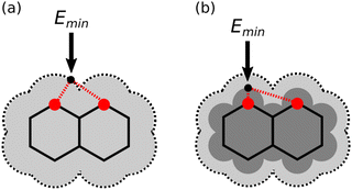
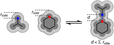
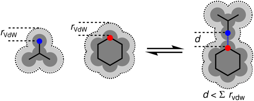
One factor that complicates the behaviour of molecules with closely packed arrays of polar groups is secondary electrostatic interactions, which are illustrated in Fig. 1. Although the two complexes are at first sight very similar, each with three intermolecular H-bonds, the association constant for formation of the complex shown in Fig. 1(a) is two orders of magnitude higher than the association constant for formation of the complex shown in Fig. 1(b) (104–105 M−1 compared with 102 M−1 in chloroform).5,6 In their classic paper,7 Jorgensen and Pranata used molecular mechanics calculations to offer an explanation. The primary H-bonding interactions shown in Fig. 1 bring neighbouring functional groups on the two molecules into close proximity. These functional groups are further apart than the H-bonded atoms, but they are close enough to make long-range secondary electrostatic interactions. Considering H-bond acceptors as atoms with partial negative charges and H-bond donors as atoms with partial positive charges provides a simple explanation for the experimental results for these systems. In Fig. 1(a), there two repulsive (red) and two attractive (blue) secondary interactions, whereas in Fig. 1(b) all the secondary interactions are repulsive. The concept of secondary electrostatic interactions has been successfully used to design exceptionally stable H-bonded arrays, which have applications in cosmetics, adhesives and surface films.8–10
 |
| | Fig. 1 Secondary electrostatic interactions in multiply H-bonded complexes. (a) Three primary H-bonding interactions (grey), two repulsive secondary electrostatic interactions (red) and two attractive secondary electrostatic interactions (blue). (b) Three primary H-bonding interactions (grey) and four repulsive secondary electrostatic interactions (red). | |
There have been many theoretical investigations of the properties of complexes with arrays of multiple H-bonds, such as those shown in Fig. 1. A large number of different factors have been identified as contributors to the overall stability of the complexes. It is clear that interactions between all of the atoms in the two molecules should be considered, and it has been shown that Brønsted–Lowry acid/base properties, π resonance assistance, polarisation, Pauli repulsion, dispersion and charge accumulation all play a role.11–17 These analyses highlight the difficulty of disentangling the properties of complexes, which contain multiple functional groups, where both through-bond polarisation and through-space effects contribute to interaction energies, and where there are multiple primary and secondary interactions that must be considered. Here we focus on simpler complexes with fewer interactions that allow more direct investigation of secondary electrostatic interactions. The approach is illustrated in Fig. 2. The complex in Fig. 2(a) provides a reference point with only one intermolecular H-bond and no significant secondary interactions. The complex in Fig. 2(b) introduces one additional secondary electrostatic interaction. Comparison of the stabilities of these two complexes therefore provides a simple quantification the secondary electrostatic interaction.
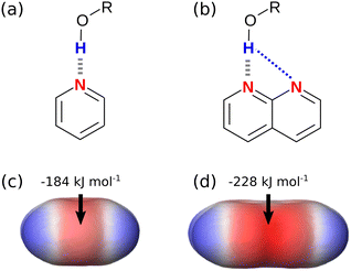 |
| | Fig. 2 (a) A complex with one intermolecular H-bond (grey). (b) A complex with one intermolecular H-bond and one attractive secondary electrostatic interaction (blue) (c) MEPS of pyridine (d) MEPS of naphthyridine. Calculations were carried out using DFT, B3LYP with a 6-31G* basis set in NWChem, and the MEPS is shown on the 0.0020 e bohr−3 electron density isosurface with the minimum value Emin highlighted. | |
We have previously shown that the properties of complexes like the one in Fig. 2(a) which have a single intermolecular H-bond can be accurately predicted using eqn (1).
| | | ΔG°/kJ mol−1 = −(α − αS)(β − βS) + 6 | (1) |
where
α and
β are H-bond donor and acceptor parameters that describe the solutes,
αS and
βS are the corresponding H-bond parameters that describe the solvent, and 6 is an empirical constant.
18
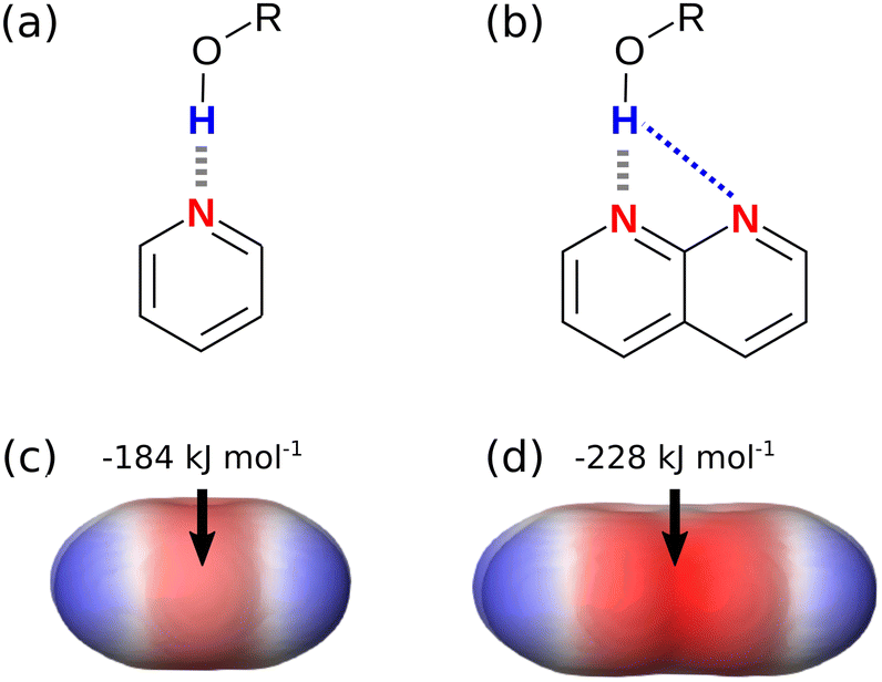
The H-bond parameters used in eqn (1) can be determined experimentally using measurements of association constants for formation of 1:1 complexes, or they can be calculated using ab initio methods. Fig. 2(c) shows the molecular electrostatic potential surface (MEPS) of pyridine calculated on the 0.0020 e bohr−3 electron density isosurface, which is an approximation of the van der Waals surface.19 The minimum on the MEPS, Emin, is located over the nitrogen lone pair, and the value can be used in eqn (2) to calculate the H-bond acceptor parameter β.4
Fig. 2(d) shows the MEPS of naphthyridine. The value of Emin is significantly more negative than the value calculated for pyridine in Fig. 2(c). When these values of Emin are used in eqn (2), the calculated values of β are 7.2 for pyridine and 10.1 for naphthyridine. Implementation of these parameters in eqn (1) would predict that the naphthyridine complex shown in Fig. 2(b) is significantly more stable than pyridine complex in Fig. 2(a). This example suggests that the MEPS of the individual molecules may provide a useful description of the effects of secondary electrostatic interactions on the stabilities of intermolecular complexes. Although it is known that through-space interactions with neighbouring functional groups affect the MEPS of a molecule, it is not clear whether the magnitude of this effect provides an accurate prediction of the magnitude of secondary electrostatic interactions.20,21 In this paper, we use experimental measurements of association constants for formation of 1:1 complexes to establish a quantitative relationship between the ab initio calculated MEPS and the free energy contribution due to secondary electrostatic interactions to the stabilities of multiply H-bonded complexes.
2 Results
Experimental measurement of secondary electrostatic interactions
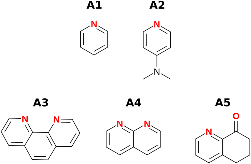
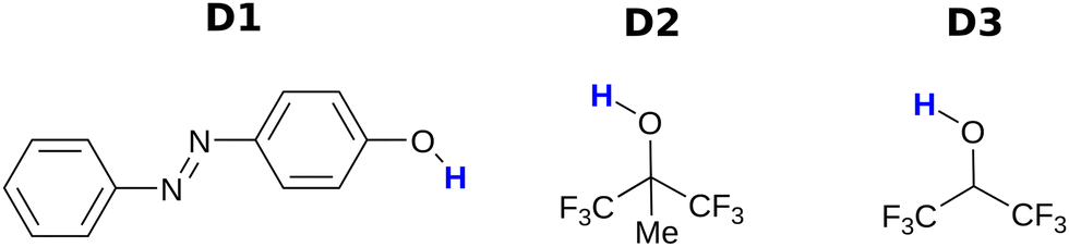
Fig. 3 and 4 show the H-bond donors and acceptors chosen for experimental investigation. Compounds A1 and A2 were used as reference points, because the experimentally determined β parameters span a wide range (7.2 to 9.3), and there are minimal secondary electrostatic interactions. Compounds A3, A4 and A5 have two H-bond acceptor sites of different polarity arranged in different geometries, which should lead to measurable secondary electrostatic interactions and allow calibration of the magnitude of through-space effects on the calculated MEPS. The presence of two interaction sites in A3 and A4 is easily taken care of, because they are identical, which leads to a statistical correction of a factor of two in the measured association constant. There could be ambiguity in the site of interaction of a H-bond donor with A5, but pyridines are much stronger H-bond acceptors than ketones, so interaction with the oxygen is unlikely.
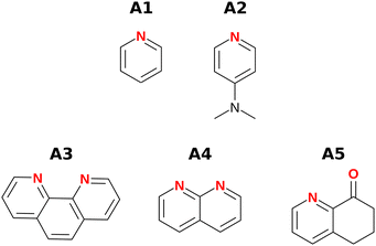 |
| | Fig. 3 H-bond acceptors. | |
 |
| | Fig. 4 H-bond donors. | |
UV/vis absorption titrations were carried out for all combinations of H-bond donors and acceptors in chlorobenzene and dichloromethane. In four cases the overlap of the absorption spectrum of the host with the spectrum of the guest or the solvent made it impossible to collect reliable data. For the other 21 systems, the data fit well to a 1:1 binding isotherm (see ESI†). The resulting association constants are presented in Table 1.
Table 1 Association constants (M−1) measured by UV/vis titrations at 298 K
|
|
Solvent |
| Chlorobenzene |
Dichloromethane |
| D1 |
D2 |
D3 |
D1 |
D3 |
|
Not determined due to spectral overlap.
|
| A1 |
99 ± 6 |
n.d.a |
n.d.a |
42 ± 3 |
94 ± 4 |
| A2 |
1070 ± 20 |
496 ± 4 |
3600 ± 200 |
480 ± 20 |
1000 ± 300 |
| A3 |
700 ± 20 |
400 ± 20 |
6300 ± 100 |
71 ± 8 |
380 ± 30 |
| A4 |
220 ± 60 |
170 ± 5 |
1630 ± 70 |
53 ± 5 |
210 ± 10 |
| A5 |
n.d.a |
68 ± 4 |
880 ± 70 |
n.d.a |
60 ± 5 |
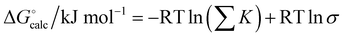
The results in Table 1 were used in eqn (1) to determine experimental values of the H-bond acceptor parameters for compounds A1–A5, βexpt. The literature values shown in Table 2 for the H-bond parameters of D1–D3 and the solvents allowed optimisation of the values of βexpt for A1–A5 to minimise the RMSE between the experimental and calculated values of ΔG°. For A3 and A4, which have two equivalent H-bond acceptor sites, the value of β was determined by applying a statistical correction to the experimentally measured association constants in Table 1.22 The optimised H-bond acceptor parameters for A1–A5 are shown in Table 2, and the agreement between the values of ΔG° calculated using these parameters and the experimentally measured values is illustrated in Fig. 5. The calculated values of ΔG° are all within 2.5 kJ mol−1 of the experimental values, with the exception of the D3·A3 complex in chlorobenzene, which is highlighted in red. An X-ray crystal structure of this complex was obtained (see ESI†). In addition to the primary OH⋯N H-bond, and there is a short contact between the CH group of the donor and the second nitrogen atom of the acceptor.23 This CH⋯N H-bond would lead to an anomalous increase the stability of this complex, and the effects would be larger in chlorobenzene, which is less polar than dichloromethane.
Table 2 H-bond parameters
|
|
α
S
|
β
S
|
α
|
β
expt
|
β
calc
|
|
Ref. 3.
The literature value in ref. 3 is 1.7, but a value of 1.6 gave much better agreement with the measurements reported here.
Ref. 25.
Ref. 26.
Agrees with ref. 24.
9.4 in ref. 24.
|
| Chlorobenzene |
1.4a |
1.1a |
— |
— |
— |
| Dichloromethane |
1.6b |
1.5a |
— |
— |
— |
|
D1
|
— |
— |
4.3c |
— |
— |
|
D2
|
— |
— |
4.0d |
— |
— |
|
D3
|
— |
— |
4.6d |
— |
— |
|
A1
|
— |
— |
— |
7.2e |
7.2 |
|
A2
|
— |
— |
— |
9.3f |
9.5 |
|
A3
|
— |
— |
— |
7.9 |
14.6 |
|
A4
|
— |
— |
— |
7.5 |
10.1 |
|
A5
|
— |
— |
— |
7.7 |
12.0 |
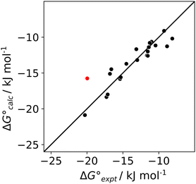 |
| | Fig. 5 Comparison of the experimental values of free energy changes for formation of 1:1 complexes ( ) with calculated values ( ) with calculated values ( ) obtained from the H-bond parameters in Table 2 and eqn (1). The line corresponds to y = x, and the D3·A3 complex in chlorobenzene is highlighted as an outlier (red point). ) obtained from the H-bond parameters in Table 2 and eqn (1). The line corresponds to y = x, and the D3·A3 complex in chlorobenzene is highlighted as an outlier (red point). | |
The values of βexpt determined for the reference compounds A1 and A2 agree exactly with the previously reported values, which gives confidence in the reliability of the measurements.24 The other three acceptors all have values of βexpt which are significantly larger than the value for pyridine (A1). This result suggests that the secondary electrostatic interactions illustrated in Fig. 2(b) do indeed enhance the stability of H-bonded complexes formed by A3–A5. Table 2 also shows values of βcalc which were obtained using eqn (2). For A1 and A2, the calculated H-bond parameters agree with experimental values. For A3–A5, the calculated H-bond parameters are much larger than the experimental values, and the size of the error depends on the arrangement of H-bond acceptor sites: the discrepancy between calculation and experiment for A3 is twice as large as the discrepancy for A4.
Computational analysis of secondary electrostatic interactions
The experiments reported here show that although the calculated MEPS of an individual molecule can be used to identify the presence of secondary electrostatic interactions in a H-bonded complex, the magnitude of the effect is overestimated if the van der Waals surface is used to calculated the electrostatic potential. Through-space effects on the MEPS can be modulated by changing the isosurface used for the calculation.21,27,28Fig. 6 illustrates the principle for A4. Fig. 6(a) shows that the minimum on the MEPS calculated on the van der Waals surface (light grey) is close to both acceptor atoms. Therefore the value of Emin is determined by a large primary contribution from the closest acceptor as well as a large secondary contribution from the other acceptor. However, the magnitude of the secondary contribution can be reduced by using a higher electron density isosurface which is closer to the nuclei (dark grey in Fig. 6(b)). In Fig. 6(b), the minimum on the dark grey surface is much closer to one of the two acceptors, and so the secondary contribution to the value of Emin from the other acceptor is small. In other words, the magnitude of through-space effects on the MEPS can be tuned by varying the electron density of the surface used for the calculation. In this way, it should be possible to find an isosurface that provides an accurate representation of the magnitudes of both primary H-bonding interactions and secondary electrostatic interactions.
 |
| | Fig. 6 Representations of electron density isosurfaces of naphthyridine. (a) On the van der Waals surface (light grey), the minimum on the MEPS (black dot) is close to both nitrogen atoms (red). (b) On a higher electron density isosurface (dark grey), the minimum on the MEPS is closer to one of the nitrogen atoms than the other. | |
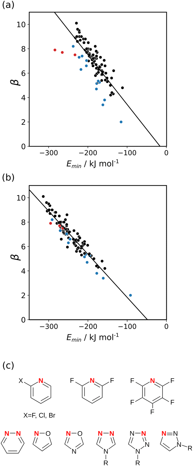
The experimentally determined H-bond acceptor parameters in Table 2 were used together with a collection of experimental parameters for compounds with sp2 nitrogen acceptors to investigate different electron density isosurfaces. For each compound, the MEPS was calculated using DFT, B3LYP with a 6-31G* basis set, at electron densities of 0.0020, 0.0050, 0.0104, 0.0200, 0.0300, 0.0400, 0.0500, 0.0600 and 0.0700 e bohr−3. Fig. 7(a) shows the relationship between the experimental values of β and the values of Emin calculated at the van der Waals surface. Although there is some correlation, there is considerable scatter in the data, and the compounds from Table 2 are clear outliers (red points). The other outliers highlighted in blue in Fig. 7(a) are the compounds shown in Fig. 7(c). These compounds all have a second H-bond acceptor in close proximity to the sp2 nitrogen, and the calculated value of the MEPS overestimates the magnitude of the through-space effect on the H-bond acceptor properties. Fig. 7(b) shows the relationship between the experimental values of β and the values of Emin calculated at a higher density isosurface. The scatter is significantly reduced, and all of the outliers now follow the same trend as the other compounds. This surface achieves the right balance of primary and secondary contributions to the value of Emin to provide an accurate quantitative description of secondary electrostatic interactions.
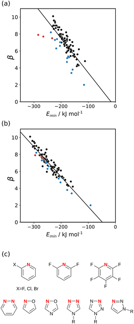 |
| | Fig. 7 Relationship between the experimentally measured H-bond parameter β for compounds with sp2 nitrogen acceptors and the value of Emin calculated using DFT, B3LYP with a 6-31G* basis set at (a) the 0.0020 e bohr−3 electron density isosurface and (b) the 0.0300 e bohr−3 electron density isosurface. The lines are the best linear fit. The points corresponding to compounds A3–A5 are highlighted in red. (c) The structures of the outliers highlighted in blue. | |
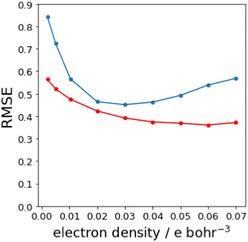
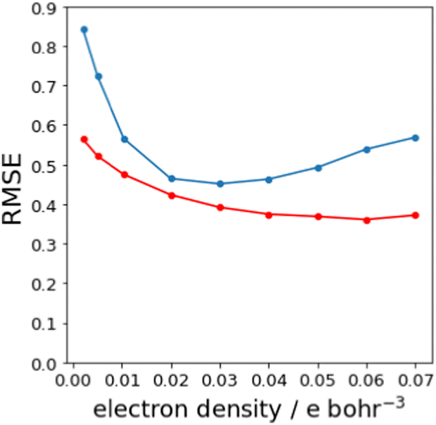
Fig. 7(b) shows that relationship between the values β and Emin is linear on the higher electron density isosurface. Therefore the values of Emin calculated at different isosurfaces were fitted to eqn (3), and the resulting values of RMSE are compared in Fig. 8 (blue data). There is a clear minimum in RMSE for isosurface densities of 0.0200 e bohr−3 to 0.0300 e bohr−3 suggesting that these surfaces provide the best description of the H-bond properties of sp2 nitrogen acceptors. The same analysis was carried out for amide carbonyl oxygen acceptors (see ESI†), and the resulting RMSE values are shown in Fig. 8 (red data). Although there is no well-defined minimum in this case, the higher density isosurfaces also provides a superior description of this class of H-bond acceptors. The 0.0300 e bohr−3 isosurface was therefore selected for calculation of β parameters using eqn (3) (sp2 nitrogen mβ = −0.036 kJ mol−1 and cβ = −1.7, amide oxygen mβ = −0.035 kJ mol−1 and cβ = 0.1).
 |
| | Fig. 8 RMSE between experimental values of β and values calculated using the best fit to eqn (3) for different electron density isosurfaces. Results for sp2 nitrogen acceptors are shown in blue, and for amide carbonyl oxygen acceptors in red. | |
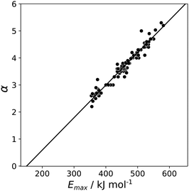
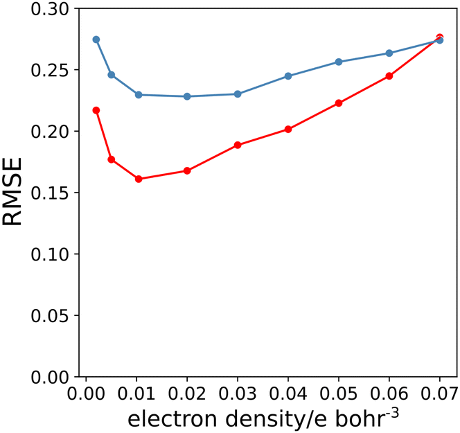
A similar approach was then used for the H-bond donor parameter α. The MEPS was calculated at different electron density isosurfaces for a collection of H-bond donors for which α parameters have been experimentally determined.4 Again higher electron density isosurfaces gave a superior description of the H-bond properties of these compounds compared with the van der Waals surface. Fig. 9 compares the experimental α parameter for OH donors with the value of Emax calculated at the 0.0104 e bohr−3 isosurface. The relationship between α and Emax is clearly linear. Therefore the values of Emax calculated at different isosurfaces were fit using eqn (4), and the resulting values of RMSE are compared in Fig. 10 (red data). There is a well-defined minimum in RMSE for an isosurface density of 0.0104 e bohr−3 suggesting that this surface provides the best description of the H-bond properties of OH donors. A similar result was obtained for NH donors (blue data in Fig. 10). The 0.0104 e bohr−3 isosurface was therefore selected for calculation of α parameters using eqn (4) (OH mα = 0.015 kJ mol−1 and cα = −3.8, NH mα = 0.011 kJ mol−1 and cα = −2.8).
 |
| | Fig. 9 Relationship between the experimentally measured H-bond parameter α for compounds with OH donors and the value of Emax calculated using DFT, B3LYP with a 6-31G* basis set at the 0.0104 e bohr−3 electron density isosurface. The line is the best linear fit. | |
 |
| | Fig. 10 RMSE between experimental values of α and values calculated using the best fit to eqn (4) for different electron density isosurfaces. Results for NH donors are shown in blue, and for OH donors in red. | |
Fig. 11 provides a rationale for the superior performance of the higher electron density isosurfaces in predicting H-bonding properties. Neutron diffraction experiments show that the distance between a H-bond acceptor and the hydrogen atom of the donor in a H-bond is shorter than the sum of the van der Waals radii by 0.5–1.0 Å.29 On the optimal electron density isosurfaces identified above, the location of Emin is 0.45 Å closer to the nucleus than the van der Waals surface and the location of Emax is 0.25 Å closer to the nucleus. These locations would represent the point of contact between two H-bonded molecules that penetrate the van der Waals surfaces by 0.7 Å, which is consistent with the experimental measurements.
 |
| | Fig. 11 Penetration of the van der Waals surface on formation of a H-bond. | |
3 Secondary electrostatic interactions in H-bond arrays
Experimentally determined association constants were collected from the literature for 37 different 1:1 complexes with multiple H-bonds measured in chloroform, dichloromethane or carbon tetrachloride.6,10,30–42 The components of these complexes are all relatively rigid molecules, so that entropy changes due to conformational restriction make minimal contributions to the free energy changes associated with complexation. The geometries of the individual molecules were optimised using DFT. For each compound, the MEPS was calculated at the 0.0020, 0.0104 and 0.0300 e bohr−3 electron density isosurfaces, and these surfaces were used to calculate H-bond parameters as explained below.
Two different methods were used to obtain H-bond parameters. In the first method, footprinting of the 0.0020 e bohr−3 electron density isosurface was used to obtain a set of surface site interaction points (SSIP), and the SSIP closest in space to each H-bond donor and acceptor group was used as the H-bond parameter for that interaction site.4,43 In the second method, eqn (3) and (4) were used in conjunction with the 0.0104 e bohr−3 and the 0.0300 e bohr−3 isosurfaces to determine H-bond parameters. Firstly, each point on the MEPS was assigned to the closest atom in space.44 The maximum value on the MEPS assigned to each H-bond donor was then used to calculate the value of α for that interaction site, and the minimum value assigned to each H-bond acceptor was used to calculate the value of β. For oxygen atoms with two well-defined minima on the MEPS, two values of Emin corresponding to the two lone pair directions were considered.45
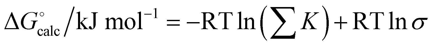
The association constant K for formation of a complex that makes N H-bonds was calculated using eqn (5). Each H-bond contributes a free energy change described by eqn (1), and an effective molarity (EM) term was added to account for the intramolecular nature of all interactions after the first intermolecular H-bond is made. The value of EM is not known, but we assume that a constant value can used for all of these systems, because the molecules are relatively rigid and the H-bond arrays have similar geometries.
| |  | (5) |
For some of the complexes used in this study, multiple binding modes are possible. For example, adenine can form doubly H-bonded complexes of similar stability along the Watson–Crick or Hoogsteen faces. The overall association constant can be obtained by summing over all possible binding modes. In addition for complexes involving self-association, a statistical factor must be included to compare with the experimentally measured free energy change.46Eqn (6) was therefore used to obtain calculated values of ΔG° for comparison with experimental data.
| |  | (6) |
where
σ is 2 for self-association and 1 for hetero-complexes.
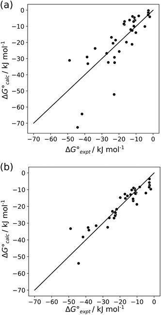
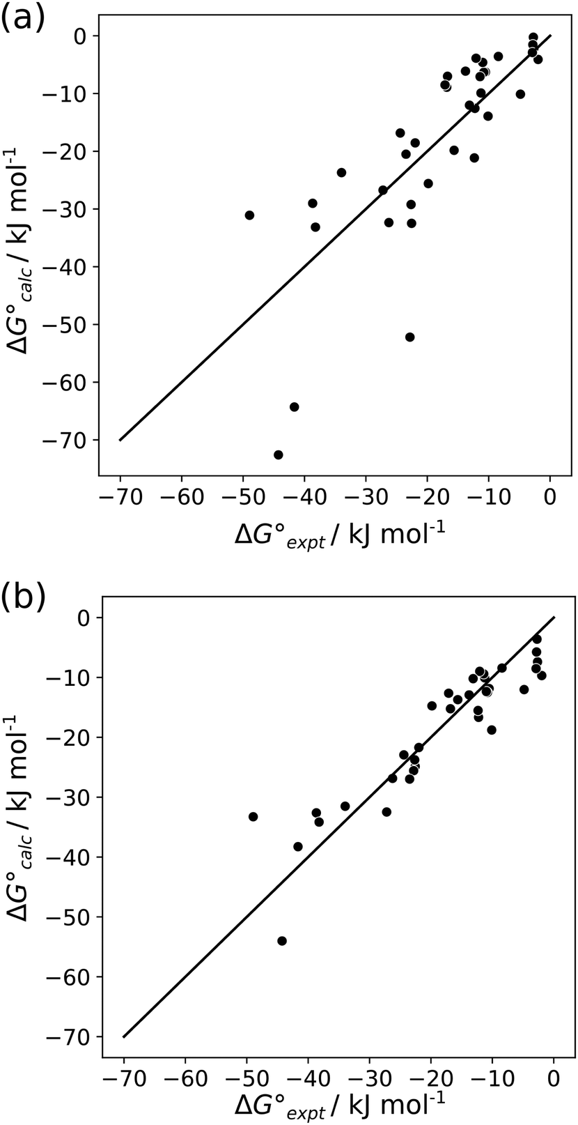
For the two different sets of H-bond parameters described above, the value of EM was optimised to minimise the RMSE between the experimental values of ΔG° and the values calculated using eqn (6). The optimised value of EM did not show any significant dependence on the method used to calculate H-bond parameters: 93 M for H-bond parameters obtained from the van der Waals surface, and 125 M for H-bond parameters obtained from the higher density isosurfaces. However, there are dramatic differences in the results obtained using the two methods. Fig. 12(a) shows that H-bond parameters obtained from the van der Waals surface provide a poor description of the properties of multiply H-bonded complexes (RMSE = 9.8 kJ mol−1). Fig. 12(b) shows that H-bond parameters obtained from the higher density isosurfaces provide a good description of these systems (RMSE = 4.7 kJ mol−1). This method also performs better than direct calculation of complexation energies using ab initio methods (see ESI† for comparison with previous reports).47
 |
| | Fig. 12 Comparison of experimentally measured free energy changes for formation of multiply H-bonded complexes ( ) with calculated values ( ) with calculated values ( ) obtained from eqn (5) and (6) and H-bond parameters calculated on (a) the van der Waals surface, and (b) at the higher electron density isosurfaces (0.0300 e bohr−3 for β and 0.0104 e bohr−3 for α). The black lines are y = x. ) obtained from eqn (5) and (6) and H-bond parameters calculated on (a) the van der Waals surface, and (b) at the higher electron density isosurfaces (0.0300 e bohr−3 for β and 0.0104 e bohr−3 for α). The black lines are y = x. | |
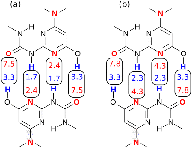
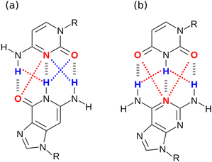
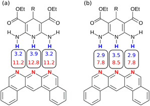
The difference in the performance of the two methods can be directly related to the treatment of secondary electrostatic interactions. Fig. 13 compares the description of an ADAD·ADAD complex using H-bond parameters derived from different surfaces. The parameters for the two external H-bonds are similar in Fig. 13(a) and (b), but the parameters for the two internal H-bonds are quite different. Secondary electrostatic interactions lower the values of the H-bond parameters for the internal sites compared with the external sites, but in both cases the effects are much larger at the van der Waals surface (Fig. 13(a)). The result is an underestimate of the stability of the calculated values for all complexes containing alternating acceptors and donors in Fig. 12(a).
 |
| | Fig. 13 H-bond parameters for an ADAD·ADAD complex calculated on (a) the van der Waals surface, and (b) the higher electron density isosurfaces (0.0300 e bohr−3 for β and 0.0104 e bohr−3 for α). | |
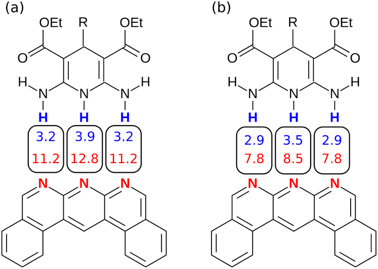
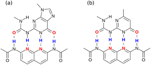
Similarly, Fig. 14 shows the H-bond parameters used to describe an AAA·DDD complex where the secondary electrostatic interactions are attractive. The H-bond donor and acceptor parameters that describe the central H-bond are elevated in both descriptions, but the effects are much larger at the van der Waals surface (Fig. 14(a)). This effect leads to an overestimate of the stability of the calculated values for all complexes containing attractive secondary electrostatic interactions in Fig. 12(a).
 |
| | Fig. 14 H-bond parameters for an AAA·DDD complex calculated on (a) the van der Waals surface, and (b) the higher electron density isosurfaces (0.0300 e bohr−3 for β and 0.0104 e bohr−3 for α). | |
The method for determining H-bond parameters using higher electron density isosurfaces clearly provides an excellent quantitative description of the secondary electrostatic interactions that determine the properties of H-bond arrays. There is one outlier in Fig. 12(b), which is the ADDA·DAAD complex shown in Fig. 15(a). This complex has a very similar structure to another ADDA·DAAD complex, which is shown in Fig. 15(b). The reported association constants are 3.8 × 10⁸ M−1 and 6 × 10⁶ M−1, but the values predicted using eqn (5) are 7 × 10⁶ M−1 for both complexes10,30 so this outlier may be an artefact. Removing this outlier reduces the RMSE for the results shown in Fig. 12(b) from 4.7 to 4.0 kJ mol−1.
 |
| | Fig. 15 ADDA·DAAD complexes. (a) K = 3.8 × 10⁸ M−1 in chloroform10 (b) K = 6 × 10⁶ M−1 in chloroform.30 | |
4 Discussion
The results shown in Fig. 12(b) demonstrate that H-bond parameters calculated from the MEPS of the individual molecules provide a quantitative description of the contributions of secondary electrostatic interactions to the stabilities of complexes that feature multiple interactions. An advantage of the approach is that these H-bond parameters include the effects of neighbouring groups due to through-bond polarisation as well as through-space electrostatic interactions. Secondary electrostatic interactions will perturb interactions with the solvent as well as interactions with the binding partner, and implementation of the H-bond parameters described here have the effects of desolvation implicitly built into the approach through eqn (5).
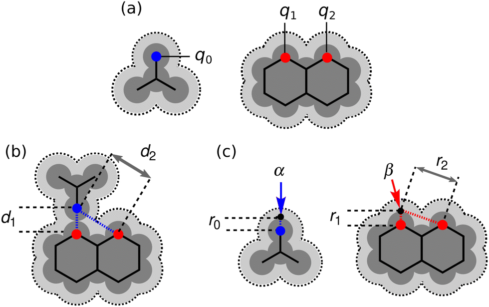
It is instructive to compare the treatment of secondary electrostatic interactions based on H-bond parameters with the original molecular mechanics interpretation. Fig. 16(a) illustrates an atom-centred point charge representation of secondary electrostatic interactions. The total Coulombic interaction E in Fig. 16(b) is the sum of the short range H-bonding interaction and the long-range secondary electrostatic interaction (eqn (7)).
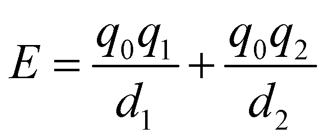
| |  | (7) |
 |
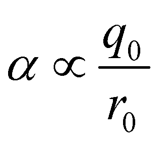
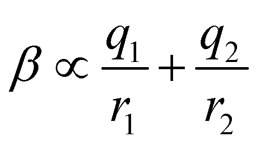
| | Fig. 16 (a) Representation of molecular charge distributions as point charges. (b) Coulombic interactions between a H-bond donor and a molecule with two H-bond acceptors. (c) The H-bond donor (α) and acceptor (β) parameters for the two compounds are proportional to the molecular electrostatic potential calculated on surfaces defined by the dark grey regions. The pale grey surfaces represent the van der Waals surface. | |
Fig. 16(c) shows how the H-bond parameters for the two compounds would be calculated using an atom-centred point charge representation of the molecular charge distribution. Since the values of α and β are linearly related to the electrostatic potential calculated at a distance r from the nucleus, which is defined by the choice of isosurface, the H-bond donor and acceptor parameters are given by eqn (8) and (9) respectively.
| |  | (8) |
| |  | (9) |
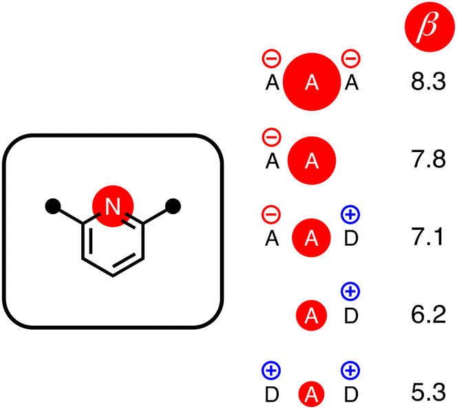
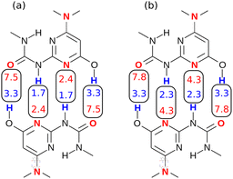
The energy associated with formation a H-bond between the two molecules is proportional to the product αβ. By multiplying eqn (8) and (9), we obtain an expression with two terms: one proportional to q0q1, which represents the primary H-bonding interaction, and one proportional to q0q2, which represents the secondary electrostatic interaction. This analysis demonstrates that the approach developed here based on the MEPS of individual molecules is exactly analogous to the original interpretation based on intermolecular electrostatic interactions developed by Jorgensen and Pranata. Indeed the qualitative ideas that stem from the original secondary electrostatic approach can be applied equally well to an approach based on H-bond parameters. Fig. 17 illustrates how the properties of H-bond arrays can be understood based on the H-bond parameters of individual molecules. The average values of the H-bond acceptor parameter β calculated for pyridine-type acceptors in different molecular environments are shown in Fig. 17. A H-bond acceptor next to the nitrogen atom increases the β value, but a neighbouring H-bond donor group decreases the β value. The effects are roughly additive, so we can think about how secondary electrostatic interactions affect the local MEPS within a molecule in just the same way as we would think about secondary electrostatic interactions between two different molecules.
 |
| | Fig. 17 The effect of secondary electrostatic interactions on the H-bond acceptor parameters of the nitrogen atoms of pyridines in different molecular environments. The value of β for unsubstituted pyridine is 7.2. | |
5 Conclusion
In this paper we have studied the through-space effects of neighbouring polar groups on the MEP at different electron density surfaces. We conclude that the effect is exaggerated at the van der Waals surface, but inner surfaces provide a much better description of the electrostatics of polar molecules. We selected the 0.0300 e bohr−3 surface for obtaining β parameters and the 0.0104 e bohr−3 surface for obtaining α parameters. Moreover, we have developed a method to predict the complexation energies of multiply hydrogen bonded systems. We show that the through-space effects at the inner surfaces quantitatively predict secondary interactions. Ultimately we show that the secondary interaction term can be obtained as an inherent property of the MEP of an individual molecule, and does not depend on the identity of the functional groups on the other molecule.
Conflicts of interest
There are no conflicts to declare.
Acknowledgements
We thank Dr A. Bond for collecting and analysing X-ray diffraction data. We thank Dr D. P. Reynolds for the stimulating discussions. We thank the Herchel Smith Fund for financial support.
Notes and references
- W. M. Latimer and W. H. Rodebush, J. Am. Chem. Soc., 1920, 42, 1419–1433 CrossRef CAS.
- L. Pauling and L. O. Brockway, Proc. Natl. Acad. Sci. U. S. A., 1934, 20, 336–340 CrossRef CAS PubMed.
- R. Cabot, C. A. Hunter and L. M. Varley, Org. Biomol. Chem., 2010, 8, 1455–1462 RSC.
- C. S. Calero, J. Farwer, E. J. Gardiner, C. A. Hunter, M. Mackey, S. Scuderi, S. Thompson and J. G. Vinter, Phys. Chem. Chem. Phys., 2013, 15, 18262–18273 RSC.
- Y. Kyogoku, R. Lord and A. Rich, Biochim. Biophys. Acta, 1969, 179, 10–17 CrossRef CAS.
- Y. Kyogoku, R. C. Lord and A. Rich, Proc. Natl. Acad. Sci. U. S. A., 1967, 57, 250–257 CrossRef CAS PubMed.
- W. L. Jorgensen and J. Pranata, J. Am. Chem. Soc., 1990, 112, 2008–2010 CrossRef CAS.
-
N. Mougin, A. Livoreil and J. Mondet, EU Pat., EP1392222B1, 2006 Search PubMed.
-
G. M. L. H. van Gemert, S. Chodorowski-Kimmes, H. M. Janssen, E. W. Meijer and A. W. Bosman, Int. Pat., WO2010002262A1, 2010 Search PubMed.
- T. Park, S. C. Zimmerman and S. Nakashima, J. Am. Chem. Soc., 2005, 127, 6520–6521 CrossRef CAS PubMed.
- P. L. A. Popelier and L. Joubert, J. Am. Chem. Soc., 2002, 124, 8725–8729 CrossRef CAS PubMed.
- W. E. V. Narváez, E. I. Jiménez, E. Romero-Montalvo, A. S. de la Vega, B. Quiroz-García, M. Hernández-Rodríguez and T. Rocha-Rinza, Chem. Sci., 2018, 9, 4402–4413 RSC.
- W. E. V. Narváez, E. I. Jiménez, M. Cantú-Reyes, A. K. Yatsimirsky, M. Hernández-Rodríguez and T. Rocha-Rinza, Chem. Commun., 2019, 55, 1556–1559 RSC.
- C.-H. Wu, Y. Zhang, K. van Rickley and J. I. Wu, Chem. Commun., 2018, 54, 3512–3515 RSC.
- A. Asensio, N. Kobko and J. J. Dannenberg, J. Phys. Chem. A, 2003, 107, 6441–6443 CrossRef CAS.
- S. C. C. van der Lubbe and C. Fonseca Guerra, Chem. – Eur. J., 2017, 23, 10249–10253 CrossRef CAS PubMed.
- W. Hujo and S. Grimme, J. Chem. Theory Comput., 2012, 9, 308–315 CrossRef PubMed.
- C. A. Hunter, Angew. Chem., Int. Ed., 2004, 43, 5310–5324 CrossRef CAS PubMed.
- R. F. W. Bader, W. H. Henneker and P. E. Cade, J. Chem. Phys., 1967, 46, 3341–3363 CrossRef CAS.
- S. C. C. van der Lubbe, F. Zaccaria, X. Sun and C. Fonseca Guerra, J. Am. Chem. Soc., 2019, 141, 4878–4885 CrossRef CAS PubMed.
- A. Oliver, C. A. Hunter, R. Prohens and J. L. Rosselló, J. Comput. Chem., 2018, 39, 2371–2377 CrossRef CAS PubMed.
- M. M. Cetin, R. T. Hodson, C. R. Hart, D. B. Cordes, M. Findlater, D. J. C. Jr., A. F. Cozzolino and M. F. Mayer, Dalton Trans., 2017, 46, 6553–6569 RSC.
- D. J. Sutor, Nature, 1962, 195, 68–69 CrossRef CAS.
- M. Berthelot, C. Laurence, M. Safar and F. Besseau, J. Chem. Soc., Perkin Trans. 2, 1998, 283–290 RSC.
- S. J. Pike, J. J. Hutchinson and C. A. Hunter, J. Am. Chem. Soc., 2017, 139, 6700–6706 CrossRef CAS PubMed.
- R. Cabot and C. A. Hunter, Org. Biomol. Chem., 2010, 8, 1943–1950 RSC.
- P. W. Kenny, J. Chem. Inf. Model., 2009, 49, 1234–1244 CrossRef CAS PubMed.
- P. W. Kenny, J. Chem. Soc., Perkin Trans. 2, 1994, 199 RSC.
- Z. Rahim and B. N. Barman, Acta Crystallogr., Sect. A: Cryst. Phys., Diffr., Theor. Gen. Crystallogr., 1978, 34, 761–764 CrossRef.
- T. F. A. de Greef, G. Ercolani, G. B. W. L. Ligthart, E. W. Meijer and R. P. Sijbesma, J. Am. Chem. Soc., 2008, 130, 13755–13764 CrossRef CAS PubMed.
- F. H. Beijer, R. P. Sijbesma, J. A. J. M. Vekemans, E. W. Meijer, H. Kooijman and A. L. Spek, J. Org. Chem., 1996, 61, 6371–6380 CrossRef CAS PubMed.
- Y. Kyogoku, R. C. Lord and A. Rich, Nature, 1968, 218, 69–72 CrossRef CAS PubMed.
- S. E. Krikorian, J. Phys. Chem., 1982, 86, 1875–1881 CrossRef CAS.
- T. J. Murray and S. C. Zimmerman, J. Am. Chem. Soc., 1992, 114, 4010–4011 CrossRef CAS.
- P. L. Wash, E. Maverick, J. Chiefari and D. A. Lightner, J. Am. Chem. Soc., 1997, 119, 3802–3806 CrossRef CAS.
- B. A. Blight, A. Camara-Campos, S. Djurdjevic, M. Kaller, D. A. Leigh, F. M. McMillan, H. McNab and A. M. Z. Slawin, J. Am. Chem. Soc., 2009, 131, 14116–14122 CrossRef CAS PubMed.
- V. Hegde, P. Madhukar, J. D. Madura and R. P. Thummel, J. Am. Chem. Soc., 1990, 112, 4549–4550 CrossRef CAS.
- R. P. Sijbesma and E. W. Meijer, Chem. Commun., 2002, 5–16 Search PubMed.
- T. W. Bell and J. Liu, J. Am. Chem. Soc., 1988, 110, 3673–3674 CrossRef CAS.
- Y. Ducharme and J. D. Wuest, J. Org. Chem., 1988, 53, 5787–5789 CrossRef CAS.
- S. H. M. Söntjens, R. P. Sijbesma, M. H. P. van Genderen and E. W. Meijer, J. Am. Chem. Soc., 2000, 122, 7487–7493 CrossRef.
- J. Hine, S. Hahn and J. Hwang, J. Org. Chem., 1988, 53, 884–887 CrossRef CAS.
- M. D. Driver, M. J. Williamson, N. D. Mitri, T. Nikolov and C. A. Hunter, J. Chem. Inf. Model., 2021, 61, 5331–5335 CrossRef CAS PubMed.
- J. L. Bentley, Commun. ACM, 1975, 18, 509–517 CrossRef.
- P. Murray-Rust and J. P. Glusker, J. Am. Chem. Soc., 1984, 106, 1018–1025 CrossRef CAS.
- C. Hunter and H. Anderson, Angew. Chem., Int. Ed., 2009, 48, 7488–7499 CrossRef CAS PubMed.
- O. Lukin and J. Leszczynski, J. Phys. Chem. A, 2002, 106, 6775–6782 CrossRef CAS.
Footnote |
| † Electronic supplementary information (ESI) available. CCDC 2170565 and 2170566. For ESI and crystallographic data in CIF or other electronic format see DOI: https://doi.org/10.1039/d2cp03004g |
|
| This journal is © the Owner Societies 2022 |
Click here to see how this site uses Cookies. View our privacy policy here. 
 Open Access Article
 This Open Access Article is licensed under a
  and
Christopher A.
Hunter
and
Christopher A.
Hunter


 ) with calculated values (
 ) obtained from the H-bond parameters in Table 2 and eqn (1). The line corresponds to y = x, and the D3·A3 complex in chlorobenzene is highlighted as an outlier (red point).
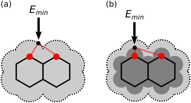


 ) with calculated values (
 ) obtained from eqn (5) and (6) and H-bond parameters calculated on (a) the van der Waals surface, and (b) at the higher electron density isosurfaces (0.0300 e bohr−3 for β and 0.0104 e bohr−3 for α). The black lines are y = x.