
 Open Access Article
 This Open Access Article is licensed under a Creative Commons Attribution-Non Commercial 3.0 Unported Licence
A physics-inspired neural network to solve partial differential equations – application in diffusion-induced stress
Yuan
Xue
a,
Yong
Li
 *a,
Kai
Zhang
b and
Fuqian
Yang
c
*a,
Kai
Zhang
b and
Fuqian
Yang
c
aJiangsu Key Laboratory of Engineering Mechanics, School of Civil Engineering, Southeast University, Nanjing, Jiangsu 210096, China. E-mail: clyong1991@seu.edu.cn
bSchool of Aerospace Engineering and Applied Mechanics, Tongji University, Shanghai 200092, China. E-mail: zhangkai@tongji.edu.cn
cMaterials Program, Department of Chemical and Materials EngineeringUniversity of Kentucky, Lexington, KY 40506, USA. E-mail: fuqian.yang@uky.edu
First published on 4th March 2022
Abstract
Analyzing and predicting diffusion-induced stress are of paramount importance in understanding the structural durability of lithium- and sodium-ion batteries, which generally require solving initial-boundary value problems, involving partial differential equations (PDEs) for mechanical equilibrium and mass transport. Due to the complexity and nonlinear characteristics of the initial-boundary value problems, numerical methods, such as finite difference, finite element, spectral analysis, and so forth, have been used. In this work, we propose two whole loss functions as the sum of the residuals of the PDEs, initial conditions and boundary conditions for the problems with decoupling and coupling between diffusion and stress, respectively, and apply a physics-inspired neural network under the framework of DeepXDE to solve diffusion-induced stress in an elastic sphere in contrast to traditional numerical methods. Using time-space coordinates as inputs and displacement and the solute concentration as outputs of artificial neural networks, we solve the spatiotemporal evolution of the displacement and the solute concentration in the elastic sphere for both the decoupling and coupling problems. The numerical results from the physics-inspired neural network are validated by analytical solutions and a finite element simulation using the COMSOL package. The method developed in this work opens an approach to analyze the stress evolution in electrodes due to electrochemical cycling.
1. Introduction
Lithium-ion batteries (LIBs), as one of the world's most promising clean energy storage devices, have attracted great attention due to their higher energy density, larger capacity, and longer life span. Diffusion-induced stress (DIS) due to the concentration gradient during mass transport and/or the deformation of active materials during charging and discharging has been proven to be one of the most important factors contributing to the failure of LIBs.1,2 DIS can be calculated generally from partial differential equations (PDEs) for mechanical equilibrium and mass transport, in which mechanical equations consist of constitutive equations and equilibrium equations and the mass transport equation is the diffusion equation. The methods to solve such a set of PDEs can follow the techniques in thermo-elasticity, as used first by Prussin.3For instance, Li4 studied DIS in elastic structures of different geometries (e.g., cylindrical, spherical and thin plate) and obtained analytical solutions for each geometry by substituting the analytical solution of the corresponding diffusion equation with the analytical solution for the corresponding thermoelastic problem. Following the thermal analogy method, Yang5 incorporated diffusion-induced bending in analyzing DIS in an elastic hollow cylinder, in which the analytical forms of resultant axial stress and hoop stress were formulated. Hao et al.6 investigated the effects of surface stress on DIS in solid and hollow nanowire electrode particles and obtained analytical solutions since the surface stress was used in the boundary conditions. Ostadhossein et al.7 studied stress effects on the initial lithiation of crystalline silicon nanowires in LIBs based on ReaxFF. Hong et al.8 used the numerical simulation in analyzing the DIS evolution in Sn micropillars.
It is very difficult to obtain analytical solutions due to the coupling between diffusion and stress with stress-assisted diffusion9 and/or a concentration-dependent elastic modulus10 being included in the DIS analysis. Similarly, it is very difficult to obtain analytical solutions when a large deformation,11–13 plastic flow,14,15 phase transition,16,17 chemical reaction,18,19 dislocation motion,20,21 and mechanical contact22 are considered in calculating the DIS in host materials of LIBs. Numerical methods, such as the finite difference method and the finite element method, are generally used to obtain numerical results. The increasing demand for fast charging has led to the observation of some critical experimental behaviors during the charging and discharging of LIBs,23,24 which require the development of numerical modeling and simulation of DIS in LIBs. However, as numerical modeling and simulation of diffusion-induced stress become more and more complex, the traditional numerical methods used to solve related PDEs may face the issues of numerical convergence and computational cost, resulting in great hindrance to research and development. Hence, there is a great need to develop new numerical methods in DIS research.
In the last decade, explosive growth of data occurred in all fields, and there has been great progress in computer-related technologies. All of these have provided the conditions needed for the development and applications of machine learning. Deep learning25–27 has become an active area in the field of machine learning and has made remarkable achievements in machine translation,28 language processing,29 visual recognition30 and other related fields. It is now convenient to use the chain rule to differentiate compositions of functions by automatic differentiation in machine learning packages, such as TensorFlow31 and PyTorch,32i.e. neural networks have become promising and efficient tools for solving PDEs.
In industrial applications of deep learning, a feedforward neural network is one of the simplest, most widely used and most rapidly developed artificial neural networks. The feedforward neural network was designed to approximate target functions, making it possible to solve PDEs by deep learning. Raissi et al.33 provided a deep learning framework, which is referred to as physics-informed neural networks (PINNs), to solve both forward problems with initial and boundary conditions and inverse problems with some additional information for nonlinear problems. Lu et al.34 proposed a deep learning library of DeepXDE and introduced a residual-based adaptive refinement method to improve the training efficiency of PINNs. Reformulating PDEs with backward stochastic differential equations, Han et al.35 targeted on solving nonlinear PDEs with hundreds and potentially thousands of dimensions. Bar-Sinai et al.36 introduced a data-driven discretization method to resolve spatiotemporal issues over large length and time scales, and their results suggested that the accuracy of the proposed method is in accordance with finite difference methods.
Solving the PDEs, which consist of geometrical equations, constitutive equations and equilibrium equations, is generally an effective way to understand the deformation and stress fields in a solid. Recently, a deep learning strategy has been used to solve mechanical problems using the strain energy of a solid as a loss function for a deep neural network.37 In analyzing the Föppl–von Kármán equation, Li et al.38 compared the differences of numerical accuracies for three differnt methods with a loss function, i.e. purely data-driven, PDE-based and energy-based. These studies suggest that deep learning likely has broad potential in solving mechanical problems and can also be applied to solve chemomechanical coupling prblems, such as DIS in LIBs.
In this work, we propose two loss functions associated with mass transport and diffusion-induced stress for decoupling and coupling between diffusion and stress, respectively, and use the loss functions in a neural network to numerically solve DIS in an elastic sphere. Such an approach is different from traditional deep learning, which needs the exact solution or reference solution at the corresponding coordinates in the training. This paper is organized as follows. In part 2, we introduce mathematical formulations for DIS and mass transport in the elastic sphere. In part 3, we briefly introduce some basic theory of deep learning and design a physics-inspired neural network, which is also referred to as the deep neural network (DNN), to solve the PDEs in part 2. In part 4, we develop three DNNs with different parameters and compare the numerical results from deep learning with analytical solutions. In part 5, we further test the robustness and capability of the DNN by analyzing DIS in the elastic sphere with stress-limited diffusion and compare the results with the results from the finite element simulation. Finally, we conclude the work.
2. Mathematical formulations for diffusion-induced stress in an elastic sphere
Consider a classical case, i.e. the DIS in an isotropic, spherical particle of an initial radius R. The deformation of the sphere is linearly elastic. Since the velocity of the elastic wave is generally much faster than the diffusion rate, mechanical deformation can be regarded as quasi-static. There are only three non-zero stress components, i.e. the radial stress component σr and tangential stress components σθ = σφ due to the spherical symmetry of the problem.Without any body force, the differential equation for the mechanical equilibrium in the elastic sphere in the framework of linear elasticity39 is
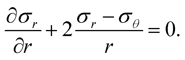 | (1) |
Similar to linear thermoelasticity,3,40 the constitutive relationship between stress and strain can be written as
 | (2) |
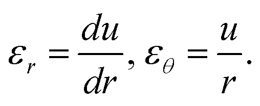 | (3) |
Substituting eqn (2) and (3) in eqn (1), we obtain the differential equation of mechanical equilibrium in terms of the radial displacement u and the solute concentration C as
 | (4) |
For the traction-free condition on the surface of the spherical particle, the initial and boundary conditions are
u(r,0) = 0,![[thin space (1/6-em)]](https://www.rsc.org/images/entities/char_2009.gif) u(0,t) = 0,σr(R,t) = 0 u(0,t) = 0,σr(R,t) = 0 | (5) |
Without the stress effects on diffusion, the differential equation for mass transport is
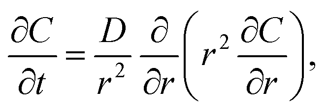 | (6) |
 | (7) |
In this work, we use time-space coordinates as the DNN inputs and the concentration and displacement as the DNN outputs. Note that there is a convergence issue for a nanosized spherical particle when the chain rule is used to differentiate the function composition via the automatic differentiation of spatial coordinates. To improve the training precision and efficiency, dimensionless variables are introduced as follows:
 | (8) |
 | (9) |
Using the dimensionless variables, eqn (4) and (6) are re-written as
 | (10) |
 | (11) |
 | (12) |
 | (13) |
3. Deep neural networks for solving PDEs
DNNs include an input layer, several hidden layers and an output layer. As one of the most basic DNNs, the feedforward neural network (FNN) is easy to be trained to solve problems in most cases. In this work, we mainly use the FNN to solve the above PDEs. Detailed information is presented in Appendix.In previous studies,35,36 most researchers had adopted a ‘data driven’ method to solve PDEs by deep learning. In the DIS analysis, using the ‘data driven’ method to deal with PDEs requires the coordinate r and time t as the inputs of a neural network and the numerical solutions of the displacement u and the concentration C as the outputs. A key part of the neural network to evaluate the results is the loss function, which can be expressed in the ‘data driven’ method as
 | (14) |
As given by eqn (14), the loss function for the data-driven model can be minimized only when the solution field of a sufficiently large number of sample points can be observed. However, for the PDEs in the DIS analysis, exact solutions or reference solutions are generally difficult to derive and/or obtain. Hence, it is necessary to develop new loss functions to obtain the solutions.
To use DNNs to solve the DIS problems, the outputs of the DNN must satisfy the PDs of (10) and (11) and the corresponding initial and boundary conditions of (12) and (13). Following the work by Lu et al.,34 we construct a whole loss function of the PDEs for the DIS in the spherical sphere as the sum of the residuals of the PDEs and the initial and boundary conditions in analyzing the discrepancy between the DNN and constraints.
Let LPDEs be the residuals from the two PDEs as
 | (15) |
The boundary conditions for mechanical deformation include the traction and displacement conditions, and both can be regarded as the Dirichlet boundary condition. For the mass-transport equation, the boundary conditions are the Neumann boundary conditions. The loss function of the initial conditions can be treated as the ones similar to the Dirichlet boundary condition in DNNs. Thus, the loss functions for the four boundary conditions LBCs and two initial conditions LICs are constructed, respectively, as
 | (16) |
 | (17) |
Here, (0, τi),(1, τi) and (xi, 0) are the residual points sampled randomly on the boundary (i.e., x = 0 and x = 1) at the initial time (i.e., τ = 0). NBCs is the number of points sampled on the left and right boundaries, and NICs is the number of points sampled at initial time.
The whole loss function is then constructed as
| LDIS = LPDEs + λ(LBCs + LICs) | (18) |
The minimization of the total loss LDIS is performed to determine the appropriate whole weight matrix and bias vector θ* = [W, b] in the DNN, which is used to obtain the numerical solution of the corresponding PDEs for the given initial and boundary conditions for a pre-determined error limit ε. When the whole loss function is smaller than the error limit, the DNN stops training and establishes the whole weight matrix and bias vector. The flow chart of the DNN with the loss functions to solve the PDEs for the DIS in the elastic sphere is shown in Fig. 1, and some parameters and optimizers used in the DNN are listed in Table 1. Note that we can pre-determine an iteration number as the stop signal instead of the error tolerance for optimization. The open-source machine learning libraries Tensorflow31 and DeepXDE34 were used in the DNN to obtain related parameters.
 | ||
| Fig. 1 Flow chart of the DNN to solve the PDEs for the DIS in the elastic sphere. | ||
According to eqn (18), the training data in this work are different from those used in the traditional ‘data driven’ method36 and possess the following pivotal features.
• The dataset does not contain exact solutions (reference solutions).
• The dataset only relies on the coordinates in the solution domain, which indicates that the number of training points can be infinite theoretically.
• The training sample can be arbitrary and can be adjusted during the training process.
Generally, the validation and test processes are important to DNNs;41,42 however, the DNN used in this work can be regarded as a computation tool in solving the PDEs rather than training a “universal” model to find the solution of any PDE. Since the dataset can be sampled arbitrarily, we only used sample 2000 points to test during iterations. Meanwhile, it should be noted that once the training is completed for the given coordinates of any point, the DNN can give the corresponding solutions. Thus, one can obtain the results of all the domains without considering the results in the test set that is a sub-domain of the whole solution domain.
4. DISs in the elastic sphere without stress-limited diffusion
The procedure for solving the PDEs by deep learning is summarized here. First, we construct a neural network û = (y;θ*) as a surrogate of the solution u(y), which takes the input y = [x, τ] and the output vector with the same dimension as u. Second, two training sets for the PDEs and initial/boundary conditions are specified. A loss function consisting of the summation of the weighted L2 norm of both the PDE equations and initial/boundary conditions is established to measure the discrepancy between the neural network û(y;θ*) and constraints. Finally, the minimization of the loss function of the DNN allows for the determination of the parameter θ*, which is referred to as the “training” process. It should be noted that there is no guarantee for a unique solution because of the nonconvex optimization problem. A common strategy is to perform random initialization a few times for the training process and choose the final solution from the solutions with the smallest training loss. In this work, all the training tasks are handled using a Nvidia Titan Rtx GPU.According to the reports in the literature,39 the number of training points and the weights of loss may heavily affect the final results. Based on the loss weights and the number of training points, we adopted three DNNs with different parameters to investigate the effects of the number of the sample points on the stress distribution and mass transport. We set the first DNN with Nd:NBCs:NICs = 10000:200:100 and λ = 1.0, the second one with Nd:NBCs:NICs = 10000:200:100 and λ = 0.1, and the third one with Nd:NBCs:NICs = 20000:400:200 and λ = 0.1. One can analyze the effect of the number of training points by comparing the results between the DNN solution with Nd = 10000 and λ = 1.0 and the DNN solution with Nd = 20000 and λ = 1.0, and from the DNN solution with Nd = 10000 and λ = 1.0 and the DNN solution with Nd = 10000 and λ = 0.1, one can determine the effect of the loss weight. It needs to be pointed out that all the training points in the domain, on the boundary and at the initial time, are chosen randomly from a uniform distribution.
All the properties of the material used in the loss function of eqn (18) are listed in Table 2, which are the material properties of the electrode material Mn2O4 used in LIBs.40 After completing the training, the DNN, we can obtain the DNN solutions of the dimensionless displacement and the concentration for the given initial and boundary conditions.
| Parameters | E | ν | Ω | J 0 | R | D | C 0 |
|---|---|---|---|---|---|---|---|
| Value | 1010 | 0.3 | 3.497 × 10⁻⁶ | 0.001 | 2.0 × 10⁻⁷ | 7.08 × 10⁻¹⁵ | 0 |
| Unit | Pa | — | m3 mol−1 | mol (m2 s)−1 | m | m2 s−1 | mol m−3 |
The numerical results obtained from the DNN with the proposed architecture and loss function are compared to the analytical solution of the corresponding problem. Without the stress-limited diffusion, the concentration distribution in the elastic sphere in a dimensionless form is45
 | (19) |
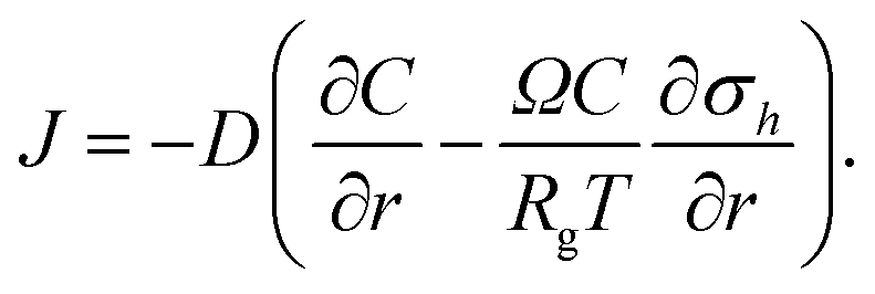
To visualize the accuracy of the prediction and analyze the error, we sampled 2000 points uniformly at several fixed times (e.g., τ = 0.01, 0.1, 0.2 and 0.4) and then plotted the DNN solutions under different parameters. For comparison, the results from the analytical solutions at these typical dimensionless times are also shown in Fig. 2. Here, the red solid lines represent the spatial distribution of the solute concentration and the displacement obtained from the analytical solutions at different dimensionless times, and the blue dashed lines, green dashed–dot lines and yellow dotted lines represent, respectively, the numerical results obtained from three different DNNs at different dimensionless times. To more intuitively compare the differences between different DNN solutions and the analytical solutions, we enlarge the plots at some key dimensionless time nodes in Fig. 2.
 | ||
| Fig. 2 Numerical results from the three different DNN solutions and the analytical solutions: (a) dimensionless concentration and (d) dimensionless displacement at dimensionless times of τ = 0.01, 0.1, 0.2 and 0.4; (b and c) enlarged view of the dimensionless concentration and (e and f) enlarged view of the dimensionless displacement at some key dimensionless times. | ||
The L2 relative error between the DNN results and the analytical solutions is calculated as
 | (20) |
 | (21) |
Here, yexact and ypred correspond to the results obtained from the analytical solutions and the DNN solutions, and N is the number of points selected in computing the L2 relative error. It should be noted that the accuracies of both the dimensionless concentration and dimensionless displacement are measured by the L2 relative error of eqn (20). We uniformly sampled 100 points from x = 0.01 to 1.0 (i.e. 0.01, 0.02, …, 0.99, 1.0), which is used to quantitatively calculate the L2 relative error between the exact solutions and DNN solutions. All the correlation coefficients of the L2 relative error under different DNN solutions are listed in Table 3. Table 3 also lists the training time under different DNN solutions.
000 and λ = 1.0, (b) DNN solution with Nd = 10000 and λ = 0.1, and (c) DNN solution with Nd = 20000 and λ = 1.0
| (a) | ||||
|---|---|---|---|---|
| τ | 0.01 | 0.1 | 0.2 | 0.4 |
| Accuracy of C* | 0.9889 | 0.9973 | 0.9984 | 0.9993 |
| Accuracy of u* | 0.9376 | 0.9801 | 0.9900 | 0.9952 |
| Training time(s) | 295 | |||
| (b) | ||||
|---|---|---|---|---|
| τ | 0.01 | 0.1 | 0.2 | 0.4 |
| Accuracy of C* | 0.9798 | 0.9952 | 0.9973 | 0.9988 |
| Accuracy of u* | 0.8951 | 0.9672 | 0.9826 | 0.9926 |
| Training time(s) | 261 | |||
| (c) | ||||
|---|---|---|---|---|
| τ | 0.01 | 0.1 | 0.2 | 0.4 |
| Accuracy of C* | 0.9998 | 0.9989 | 0.9992 | 0.9997 |
| Accuracy of u* | 0.5976 | 0.9307 | 0.9784 | 0.9835 |
| Training time(s) | 443 | |||
It can be observed from Fig. 2a that the red solid lines, blue dashed lines, green dash–dot lines and yellow dotted lines at different dimensionless times nearly overlap, suggesting that the DNN successfully predicts the concentration distribution. Such a result is also confirmed in Table 3, as the correlation coefficients of the L2 relative error for the dimensionless concentration at different dimensionless times are approximately equal to 1. According to Fig. 2d, the red solid lines, blue dashed lines, green dash–dot lines and yellow dotted lines at dimensionless times τ = 0.01 and 0.4 nearly overlap; however, the red lines slightly deviate from the results from the DNN solutions at dimensionless times τ = 0.01 and 0.1, leading to the L2 relative error of the dimensionless displacement at dimensionless times τ = 0.01 and 0.1 larger than those of the corresponding ones at τ = 0.2 and 0.4. The numerical results from the DNN solutions have slight errors in predicting the spatial distribution of the dimensionless displacement at dimensionless times τ = 0.01 and 0.1, while the numerical results from the DNN solutions are still acceptable.
According to Fig. 2 and Table 3, we can conclude that the DNN solution with Nd = 10000 and λ = 1.0 gave the best results with the least training time and the DNN solution with Nd = 20000 and λ = 1.0 took the longest training time and had the worst results. For the DNN solution with Nd = 20000 and λ = 1.0 at τ = 0.01, the relative error of the dimensionless displacement is very large because the exact dimensionless displacement is close to 0. In fact, this is a common behavior in the training process of the DNN, which is referred to as “overfitting”.46
The analytical solutions of the radial and hoop stresses are calculated from the theory of elasticity39 with eqn (10) and the initial/boundary conditions (12). Using eqn (19), we have the DIS in the elastic sphere as
 | (22) |
 | (23) |
Note that the dimensionless concentration and dimensionless displacement are the outputs of the DNN solutions. We used the dimensionless concentration, the dimensionless displacement and the constitutive relationship to calculate the DIS in the elastic sphere. The dimensionless stresses in the elastic sphere are
 | (24) |
 | (25) |
In the following discussion, we use the dimensionless concentration and dimensionless displacement obtained from the DNN solution with Nd = 10000 and λ = 1.0. Fig. 3 shows the spatial distribution of the dimensionless radial and hoop stresses at four dimensionless times τ = 0.01, 0.1, 0.2 and 0.4. Solid lines represent the numerical results from the analytical solution, and dashed lines represent the numerical results obtained from the DNN solution. It is evident that the solid lines and the dashed lines nearly overlap at different dimensionless times, suggesting that the DNN solution exhibits a high accuracy in calculating the DIS in the elastic sphere.
 | ||
| Fig. 3 Spatial distribution of the dimensionless radial and hoop stresses at four dimensionless times τ = 0.01, 0.1, 0.2 and 0.4. (a and b) radial stresses and (c and d) hoop stresses. | ||
It needs to be pointed out that the numerical results obtained from the DNN solution exhibit sharp increases for the radial and hoop stresses at the spherical center. In the numerical calculation, the term u/r (hoop strain) will numerically approach infinity as r approaches 0, leading to the sharp increase of the spatial distribution of radial and hoop stresses near the electrode center. In general, the numerical results obtained from the DNN solution are in good accordance with the results from the analytical solution. The difference between the numerical results obtained from the DNN solution and the results from the analytical solution decreases with an increase in the diffusion time, which indicates that the DNN gradually ‘learns’ how to solve the PDEs.
5. DISs in the elastic sphere with stress-limited diffusion
One of the important features of the DNN is the capability of solving nonlinear problems. In this section, we incorporate the stress-limited diffusion in mass transport.47 Yang9 reviewed the interaction between chemical stress and diffusion, which includes hydrostatic stress in the chemical potential. In an ideal solid solution, chemical potential μ can be expressed as| μ = μ0 + RgTlnC − Ωσh, | (26) |
 | (27) |
The species flux J can be calculated as
 | (28) |
Substituting eqn (26) in (28) yields
 | (29) |
According to the mass conservation, there is
 | (30) |
Substituting eqn (29) in (30), we have
 | (31) |
Finally, the diffusion equation considering the effect of hydrostatic stress can be obtained by substituting eqn (27) in (31).
 | (32) |
Similar to the case of Fick's diffusion under the galvanostatic operation with a constant flux J0 at the surface of the spherical particle, the initial and boundary conditions take the forms
| C(r, 0) = 0 | (33) |
 | (34) |
 | (35) |
Here, we set T = 300 K in the calculation. Other material parameters used in this section are listed in Table 2.
The effect of the stress-limited diffusion is explicitly expressed in the differential equation for the mass transport, as revealed in eqn (31) and the corresponding boundary conditions of (32). Using the same dimensionless variables in eqn (8), eqn (32)–(35) are expressed as
 | (36) |
| C*(r, 0) = 0 | (37) |
 | (38) |
 | (39) |
Similar to the case of Fick's diffusion, the whole loss function of PDEs is calculated as the sum of the residuals of the PDEs and initial and boundary conditions, LDIS = LPDEs + λ(LBCs + LICs), with LICs the same as the case without the stress-limited diffusion and
 | (40) |
 | (41) |
The procedure for solving the PDEs with the stress-limited diffusion by the DNN is similar to that discussed in Section 4, except the change of the whole loss function with eqn (40) and (41). Three DNNs with the same parameters as Fick's diffusion are used. The numerical results obtained from the DNN solutions are compared to the numerical results from the finite element simulation (FEM) to evaluate the accuracy of the DNN solutions. The PDE module in the commercial multi-physics software of COMSOL was used in the finite element simulation. The 2-node linear element with an element length of R0/1000 was used to ensure the convergence and accuracy of the FEM results. Note that there is no analytical solution for the nonlinear diffusion eqn (32) with the initial and boundary conditions (33)–(35).
Fig. 4 shows the spatial distributions of the dimensionless concentration and dimensionless displacement at four dimensionless times τ = 0.01, 0.1, 0.2 and 0.4. The red solid lines represent the spatial distribution of the FEM results of the dimensionless concentration and dimensionless displacement at different dimensionless times, and the blue dashed lines, green dashed–dot lines and yellow dotted lines represent the numerical results obtained from three DNNs with different parameters at different dimensionless times. The correlation coefficients of the L2 relative error, as listed in Table 4, are also used to analyze the accuracy of the numerical results obtained from the DNN solutions.
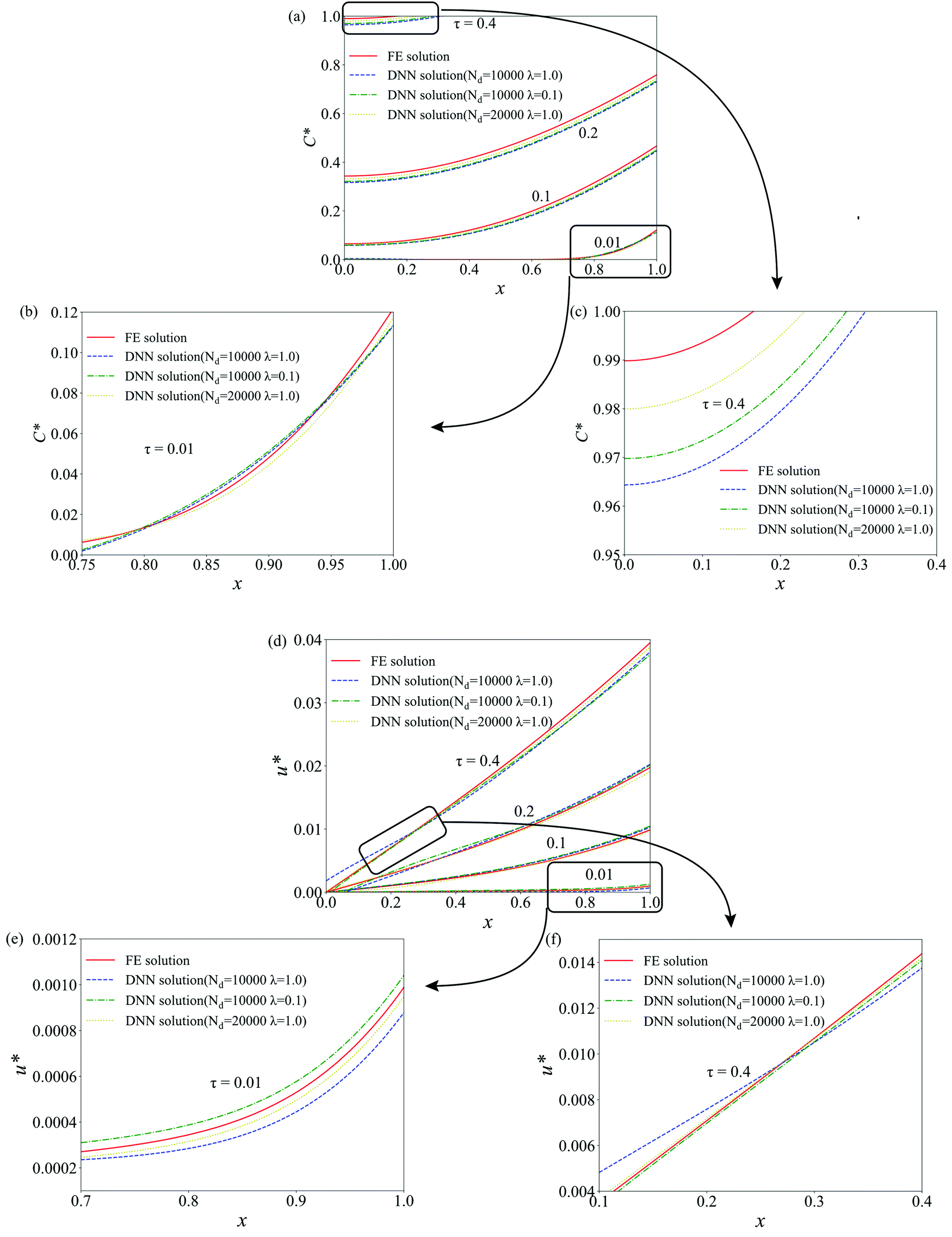 | ||
| Fig. 4 Numerical results from the DNN solutions with different parameters and the FEM simulation: (a) dimensionless concentration and (d) dimensionless displacement at dimensionless times of τ = 0.01, 0.1, 0.2 and 0.4; (b and c) enlarged view of the dimensionless concentration and (e and f) enlarged view of the dimensionless displacement at some key dimensionless times. | ||
According to Fig. 4, the red solid lines, blue dashed lines, green dashed–dot lines and yellow dotted lines at different dimensionless times nearly overlap, suggesting that the DNN solutions successfully obtain the spatial distributions of the solute concentration and the displacement. As listed in Table 4, the L2 relative error of the dimensionless concentration at different dimensionless times increases slightly with the increase of the dimensionless time and are larger than the corresponding one without the coupling effect. Such a trend in the L2 relative error of the dimensionless concentration is likely due to the coupling between stress and diffusion, leading to the increase in the numerical error. A similar conclusion can be drawn from the L2 relative error of the dimensionless displacement at different dimensionless times, i.e. the accuracy is lower than the corresponding one without the coupling effect.
000 and λ = 1.0, (b) DNN solution with Nd = 10000 and λ = 0.1, and (c) DNN solution with Nd = 20000 and λ = 1.0
| (a) | ||||
|---|---|---|---|---|
| τ | 0.01 | 0.1 | 0.2 | 0.4 |
| Accuracy of C* | 0.9256 | 0.9257 | 0.9402 | 0.9693 |
| Accuracy of u* | 0.8092 | 0.9165 | 0.9398 | 0.9561 |
| Training time(s) | 166 | |||
| (b) | ||||
|---|---|---|---|---|
| τ | 0.01 | 0.1 | 0.2 | 0.4 |
| Accuracy of C* | 0.9264 | 0.9291 | 0.9443 | 0.9714 |
| Accuracy of u* | 0.8738 | 0.9423 | 0.9558 | 0.9603 |
| Training time(s) | 160 | |||
| (c) | ||||
|---|---|---|---|---|
| τ | 0.01 | 0.1 | 0.2 | 0.4 |
| Accuracy of C* | 0.9583 | 0.9648 | 0.9762 | 0.9937 |
| Accuracy of u* | 0.9465 | 0.9534 | 0.9659 | 0.9864 |
| Training time(s) | 272 | |||
For three different DNN solutions, the DNN solution with Nd = 20000 and λ = 1.0 provides the best results in contrast to the case without coupling. Note that the accuracy may increase slightly if we use more training points (e.g., 50000 points in the solution domain). However, this will significantly increase the training time with a slight increase in the accuracy (e.g., from 0.9998 to 0.9999).
Using the numerical results of the dimensionless concentration and dimensionless displacement obtained from the DNN solution with Nd = 20000 and λ = 1.0, we calculated the DIS in the elastic sphere with the coupling between diffusion and stress. Fig. 5 displays the spatial distributions of the dimensionless radial and hoop stresses at four dimensionless times τ = 0.01, 0.1, 0.2 and 0.4. Solid lines represent the FEM results, and the dashed line represents the numerical results calculated from the DNN solutions. According to Fig. 5, the numerical results from the DNN solutions exhibit sharp increases of the radial and hoop stresses at the spherical center, the same as the case without the coupling. Also, the dashed lines deviate slightly from the solid lines at different dimensionless times near the surface of the elastic sphere in contrast to the case without the coupling. This behavior reveals that the coupling between stress and diffusion introduces a slightly larger error than the case without the coupling.
 | ||
| Fig. 5 Spatial distribution of the dimensionless radial and hoop stresses at four dimensionless times τ = 0.01, 0.1, 0.2 and 0.4. (a and b) radial stresses; (c and d) hoop stresses. | ||
6. Conclusions
In summary, we have demonstrated the feasibility of using DNNs to solve the DIS problems in a spherical electrode of LIBs with two whole loss functions for the cases with and without the coupling between stress and diffusion, respectively. The two whole loss functions were developed under the framework of linear elasticity for DIS in an elastic sphere. Three different DNNs with different parameters were used in the training of the DNN, and the numerical results obtained from the DNN solutions were compared to those from the exact solutions and the FEM results, respectively. The results reveal that we can use the DNN and the whole loss functions to analyze the DIS present in the elastic sphere during electrochemical cycling.DNNs have the following advantages over traditional numerical methods in solving the DIS problems in elastic materials.
• The DNN is a mesh-free method that can reduce the error introduced by meshing to ensure a certain accuracy.
• The DNN can handle two PDEs in DIS problems simultaneously, which can limit the errors introduced in the substitution process.
• Once the DNN for solving the PDEs in DIS problems has been designed, we only need to change some parameters (e.g., boundary conditions and initial conditions) to solve similar problems, which saves the calculation time.
Compared with the traditional DNN method – ‘data driven’, the method presented in this work does not rely on any exact solution, which means it can be implemented to solve the practical DIS problems because the exact solutions are very difficult to obtain. It needs to be pointed out that more training points are needed to reduce the “overfitting” behavior and increase the accuracy. However, there is only a slight increase in the accuracy with increasing the training. There is a great need to design DNNs with less training time, strong adaptability and high accuracy.
Author contributions
Yuan Xue performed the deep learning calculation and wrote the manuscript; Yong Li contributed to the conception of the study; Kai Zhang performed data analyses; Fuqian Yang helped in performing the analysis with constructive discussion.Conflicts of interest
There are no conflicts to declare.Appendix. Structure of neural networks
The FNN is also referred to as a multilayer perceptron (MLP) because it has multiple hidden layers. Consider an L-layer neural network or an (L – 1) hidden-layer neural network with Sl neurons in the l-th layer. Let Snm be the m-th neuron in the n-th layer, which can be regarded as one of the outputs of the upper layer that can be obtained by applying an activation function at the upper layer Sn−1 as | (42) |
| Sl = σ(WTSl−1 + bl) | (43) |
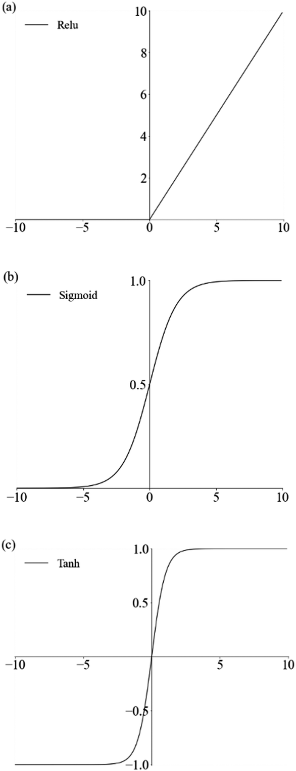 | ||
| Fig. 6 Activation functions: (a) rectified linear unit (ReLU), (b) logistic sigmoid, and (c) hyperbolic tangent (Tanh) | ||
We set x and τ as the inputs of the neural network in the DNN and u* and C* as the outputs. The hyperbolic (tanh) function is used as the activation function in the calculation. The whole neural network used to solve the PDEs can be simply expressed as
| Input layer: S0(y) = [x, τ] ∈ R2 | (44) |
| Hidden layers: Sl(y) = σ(WTSl−1(y) +bl) ∈ RSl, for 1 ≤l ≤ L −1 | (45) |
| Output layer: SL(y) = [u*, C*] ∈ R2 | (46) |
The training process is essentially to find the most appropriate weights and bias of the whole neural network by minimizing the loss function. To achieve this purpose, backpropagation48 is an important step, in which the most commonly used method is the gradient descent method.49 In addition, some common optimizers, such as stochastic gradient descent (SGD), Adam,43 and L-BFGS,44 are adopted in most cases as well.
Acknowledgements
Y. L. and K. Z. are grateful for support from the National Natural Science Foundation of China under grant numbers 11902073 and 11902222.References
- F. Yang, J. Electrochem. Soc., 2021, 168, 040520 CrossRef CAS.
- P. Huang and Z. Guo, Mech. Mater., 2021, 157, 103843 CrossRef.
- S. Prussin, J. Appl. Phys., 1961, 32, 1876–1881 CrossRef CAS.
- J. C.-M. Li, Metall. Trans. A, 1978, 9, 1353–1380 CrossRef.
- F. Yang, Mech. Res. Commun., 2013, 51, 72–77 CrossRef.
- F. Hao, X. Gao and D. Fang, J. Appl. Phys., 2012, 112, 103507 CrossRef.
- A. Ostadhossein, E. D. Cubuk, G. A. Tritsaris, E. Kaxiras, S. Zhang and A. C. van Duin, Phys. Chem. Chem. Phys., 2015, 17, 3832–3840 RSC.
- C. S. Hong, N. Qaiser, H. G. Nam and S. M. Han, Phys. Chem. Chem. Phys., 2019, 21, 9581–9589 RSC.
- F. Yang, Mater. Sci. Eng., A, 2005, 409, 153–159 CrossRef.
- F. Yang, Sci. China: Phys., Mech., 2012, 55, 955–962 CAS.
- K. Zhao, M. Pharr, S. Cai, J. J. Vlassak and Z. Suo, J. Am. Ceram. Soc., 2011, 94, s226–s235 CrossRef CAS.
- Z. Cui, F. Gao and J. Qu, J. Mech. Phys. Solids, 2012, 60, 1280–1295 CrossRef CAS.
- Z. Cui, F. Gao and J. Qu, J. Mech. Phys. Solids, 2013, 61, 293–310 CrossRef CAS.
- Y. Li, W. Mao, Q. Zhang, K. Zhang and F. Yang, J. Electrochem. Soc., 2020, 167, 040518 CrossRef CAS.
- Y. Li, Q. Zhang, K. Zhang and F. Yang, J. Power Sources, 2020, 457, 228016 CrossRef CAS.
- C. V. Di Leo, E. Rejovitzky and L. Anand, J. Mech. Phys. Solids, 2014, 70, 1–29 CrossRef CAS.
- F. Gao and W. Hong, J. Mech. Phys. Solids, 2016, 94, 18–32 CrossRef CAS.
- B. Lu, Y. Song, Q. Zhang, J. Pan, Y. T. Cheng and J. Zhang, Phys. Chem. Chem. Phys., 2016, 18, 4721–4727 RSC.
- F. Yang, J. Appl. Phys., 2010, 107, 103516 CrossRef.
- Y. Li, J. Zhang, K. Zhang, B. Zheng and F. Yang, Int. J. Plast., 2018, 115, 293–306 CrossRef.
- F. Yang, Theor. Appl. Mech. Lett., 2014, 4, 051001 CrossRef.
- B. Lu, Y. Zhao, J. Feng, Y. Song and J. Zhang, J. Power Sources, 2019, 440, 227115 CrossRef CAS.
- E. Gao, B. Lu, Y. Zhao, J. Feng, Y. Song and J. Zhang, J. Electrochem. Soc., 2021, 168, 060549 CrossRef CAS.
- Y. Liu, Y. Zhu and Y. Cui, Nat. Energy, 2019, 4, 540–550 CrossRef.
- Y. Bengio, Learning deep architectures for AI, Now Publishers Inc, 2009 Search PubMed.
- L. Deng and D. Yu, Found. Trends Signal Process., 2014, 7, 197–387 CrossRef.
- Y. Bengio, A. Courville and P. Vincent, IEEE Trans. Pattern Anal. Mach. Intell., 2013, 35, 1798–1828 Search PubMed.
- A. Vaswani, S. Bengio, E. Brevdo, F. Chollet, A. N. Gomez, S. Gouws, L. Jones, Ł. Kaiser, N. Kalchbrenner and N. Parmar, Proceedings of the 13th Conference of the Association for Machine Translation in the Americas, Boston, 2018 Search PubMed.
- Y. LeCun, Y. Bengio and G. Hinton, Nature, 2015, 521, 436–444 CrossRef CAS PubMed.
- I. Goodfellow, Y. Bengio and A. Courville, Deep learning, MIT press, 2016 Search PubMed.
- M. Abadi, P. Barham, J. Chen, Z. Chen, A. Davis, J. Dean, M. Devin, S. Ghemawat, G. Irving and M. Isard, OSDI’16: Proceedings of the 12th USENIX conference on Operating Systems Design and Implementation, Savannah, 2016 Search PubMed.
- A. Paszke, S. Gross, S. Chintala, G. Chanan, E. Yang, Z. DeVito, Z. Lin, A. Desmaison, L. Antiga and A. Lerer, In NIPS Workshop, 2017 Search PubMed.
- M. Raissi, P. Perdikaris and G. E. Karniadakis, J. Comput. Phys., 2019, 378, 686–707 CrossRef.
- L. Lu, X. Meng, Z. Mao and G. E. Karniadakis, SIAM Rev., 2021, 63, 208–228 CrossRef.
- J. Han, A. Jentzen and E. Weinan, Proc. Natl. Acad. Sci. U. S. A., 2018, 115, 8505–8510 CrossRef CAS PubMed.
- Y. Bar-Sinai, S. Hoyer, J. Hickey and M. P. Brenner, Proc. Natl. Acad. Sci. U. S. A., 2019, 116, 15344–15349 CrossRef CAS PubMed.
- E. Samaniego, C. Anitescu, S. Goswami, V. M. Nguyen-Thanh, H. Guo, K. Hamdia, X. Zhuang and T. Rabczuk, Comput. Method Appl. M., 2020, 362, 112790 CrossRef.
- W. Li, M. Z. Bazant and J. Zhu, Comput. Method Appl. M., 2021, 383, 113933 CrossRef.
- S. Timoshenko and J. N. Goodier, Theory of Elasticity, Mcgraw-Hill College, Blacklick, OH, 1970 Search PubMed.
- F. Hao and D. Fang, J. Electrochem. Soc., 2013, 160, A595–A600 CrossRef CAS.
- D. Kang, X. Wang, X. Zheng and Y.-P. Zhao, Fuel, 2021, 290, 120006 CrossRef CAS.
- J. Ma, D. Kang, X. Wang and Y.-P. Zhao, Fuel, 2022, 310, 122250 CrossRef CAS.
- O. Konur, D. Kingma and J. Ba, International Conference on Learning Representations, San Diego, 2015 Search PubMed.
- R. H. Byrd, P. Lu, J. Nocedal and C. Zhu, SIAM J. Sci. Comput., 1995, 16, 1190–1208 CrossRef.
- J. Crank, The mathematics of diffusion, Oxford university press, 1979 Search PubMed.
- N. Srivastava, G. Hinton, A. Krizhevsky, I. Sutskever and R. Salakhutdinov, J. Mach. Learn. Res., 2014, 15, 1929–1958 Search PubMed.
- Y. Li, K. Zhang and B. Zheng, Solid State Ionics, 2015, 283, 103–108 CrossRef CAS.
- D. E. Rumelhart, G. E. Hinton and R. J. Williams, Nature, 1986, 323, 533–536 CrossRef.
- S. Klein, J. P. Pluim, M. Staring and M. A. Viergever, Int. J. Comput. Vis., 2009, 81, 227 CrossRef.
| This journal is © the Owner Societies 2022 |