
 Open Access Article
 This Open Access Article is licensed under a
 Creative Commons Attribution 3.0 Unported Licence
Dynamic stabilisation during the drainage of thin film polymer solutions†
Emmanouil
Chatzigiannakis
 and
Jan
Vermant
*
and
Jan
Vermant
*
Department of Materials, ETH Zürich, 8032 Zürich, Switzerland. E-mail: jan.vermant@mat.ethz.ch
First published on 8th April 2021
Abstract
The drainage and rupture of polymer solutions was investigated using a dynamic thin film balance. The polymeric nature of the dissolved molecules leads to significant resistance to the deformation of the thin liquid films. The influence of concentration, molecular weight, and molecular weight distribution of the dissolved polymer on the lifetime of the films was systematically examined for varying hydrodynamic conditions. Depending on the value of the capillary number and the degree of confinement, different stabilisation mechanisms were observed. For low capillary numbers, the lifetime of the films was the highest for the highly concentrated, narrowly-distributed, low molecular weight polymers. In contrast, at high capillary numbers, the flow-induced concentration differences in the film resulted in lateral osmotic stresses, which caused a dynamic stabilisation of the films and the dependency on molecular weight distribution in particular becomes important. Phenomena such as cyclic dimple formation, vortices, and dimple recoil were observed, the occurrence of which depended on the relative magnitude of the lateral osmotic and the hydrodynamic stresses. The factors which lead to enhanced lifetime of the films as a consequence of these flow instabilities can be used to either stabilise foams or, conversely, prevent foam formation.
1 Introduction
When bubbles or droplets come into close proximity, a thin liquid film (TLF) usually forms between them. The dynamics of this TLF control both the equilibrium1 and non-equilibrium2 properties of various multiphase systems, such as foams, emulsions, antibubbles, and immiscible polymer blends.3–7 A body of work related to the dynamics of TLFs has focused on the influence of the interaction forces and surface stresses on film stability.8–10 For example, the effects of DLVO forces acting across the film have been quantified,11,12 and effects of surface rheology,13,14 and Marangoni stresses15–17 on the drainage have been studied for a wide range of surface-active systems. Yet, properties of the bulk fluids in confinement have also been identified as possibly playing an important role.18–21 The most known effect is the occurrence of oscillatory structural forces normal to the interface due the confinement of finite sized structural elements, such as micelles,22 nanoparticles18 or polyelectrolytes.23 The local structuring causes a difference in the osmotic pressure between the film and the surrounding plateau border which can balance the Laplace pressure difference and stabilises the film.18 However, the expulsion of a structured layer can also gives rise to attractive depletion forces (Casimir-like forces) which accelerate drainage.24These effects have some common characteristics among different systems, like micelles, nanoparticles, and polyelectrolytes. First, the magnitude of structural forces increases with the concentration.18,22,25–27 Moreover, smaller sizes lead to larger structural forces,26,28 with size polydispersity adversely impacting film stability.18,29–31 For films at equilibrium, this reduction in film stability is attributed to the weakening of the layering in the TLF,32 while for draining films the different depletion layer lengths play a role.29 Finally, there have been some reports on polyelectrolytes and micelles, which indicate that structural forces depend on the deformability of the confined species,27,33 and on their charge density.33,34
Structural and depletion forces do not depend only on the intrinsic properties of the confined species and concentration. Rather, the observation of oscillatory forces, as measured in colloidal-probe AFM, was found to depend on the employed approach speed,27 with the importance of structural forces becoming negligible as hydrodynamics become important.29 At high drainage speeds, the deformability of the confining film surfaces also plays a role, as it results in a less constrained organisation of the confined species.35,36
One common feature is that these forces, either repulsive or attractive, act normal to the film's surface. However, lateral forces can also be induced, e.g. as the concentration of confined species in the film becomes increasingly inhomogeneous at faster thinning rates, corresponding to high Péclet numbers. This effect can be expected to occur especially in films containing poly-disperse species. In contrast to Marangoni surface stresses,16 such dynamic osmotic stresses are bulk stresses. The utilisation of such stresses to influence film drainage has not yet been explored. However, there are indications in literature that this is a worthwhile avenue. For example, it has been observed that concentration differences between the inner TLF and the surrounding Plateau border can give rise to an “osmotic swelling” of the dimple, caused by the inflow of liquid towards the centre of the film.37,38 Moreover, looking back at the pioneering work of Nikolov and Wasan,18 one can observe that the surfaces of draining films containing nanoparticles show thickness corrugations. This is another indication that apart from the normal contribution of osmotic pressure, there might be a lateral ones too, when concentration gradients are induced by the flow.
Most of the studies mentioned so far involved either the approach of bubbles or particles at constant speed and the measurement of the static oscillatory forces29,39,40 or planar films draining with very low thinning velocities.18,30 In such experimental conditions it would be impossible to detect dynamic effects such as the “osmotic swelling of the dimple”,37,41 similarly to the inability to detect using colloidal-probe AFM27 the spontaneously growing dimple due to Marangoni counterflows.42–44 Such effects can only be observed in (i) constant pressure experiments, and (ii) at realistically high capillary numbers, at which the film is dimpled.
The present work aims to investigate the conditions under which such stresses because of concentration fluctuations, which we will term dynamic osmotic stresses, come into play. This bears relevance as polymers in solution are used as viscosity modifiers, e.g. in lubricants45 where undesired foaming can be an issue46 or in emulsion stability.47 Browne48 studied the collision of two air bubbles in aqueous polyvinlypyrrolidone solutions using AFM. No structural or depletion forces were observed. Starting from such a reference case for which osmotic stresses are negligible, we then explore how and when these come into play, specifically interrogating the effect of polymer molecular weight, molecular weight polydispersity, and thinning velocity on their magnitude. We study neutral polymers, which in contrast to ref. 48 have no surface activity. We can thus decouple the effects related to the dynamic osmotic stresses from those related to Marangoni stresses and surface rheology. A good solvent for the dissolved polymer is chosen to ensure that phase separation does not occur at rest.
Using the dynamic thin film balance49 we study the behaviour of dilute and semi-dilute polymer solutions in a broad range of hydrodynamic conditions. The visualisation capabilities of this technique provides insight into the phenomena occurring in these confined environments, and provide clear guidelines for optimising the formulations of various polymer-containing industrial products, such as foams, emulsions, and lubricants.
2 Theoretical background
The dynamics of TLFs containing non-surface active polymer solutions are controlled by an interplay between hydrodynamics, capillarity, and osmotic effects. Here, we provide a brief description of these effects, specifically focusing on how osmotic stresses can arise both in the normal, as well in the lateral direction.The drainage of TLFs with deformable surfaces is usually described by the generalised Stokes–Laplace–Reynolds equation50,51 which describes the evolution of the changes in film thickness h, as a function of radial position relative to the center (r) and time (t):
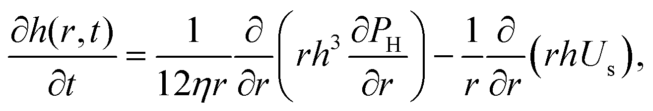 | (1) |
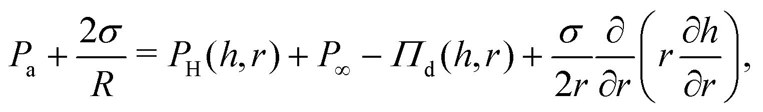 | (2) |
Eqn (1) describes the thickness profile that develops in the TLF because of flow. A dimple typically occurs as a result of an interplay between hydrodynamics and capillarity,51 which can be described by the dimensionless Capillary number,10,53 defined here based on the film characteristics:
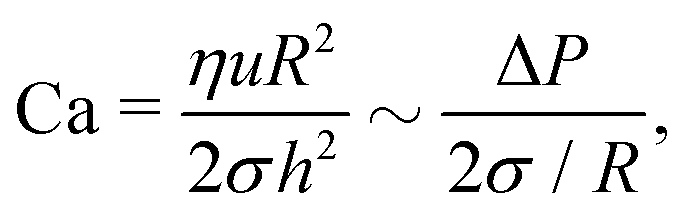 | (3) |
In the polymer solution films, Πd is equal to the sum of attractive the van der Waals interactions (ΠvdW), and the osmotic forces (Πosm). Πd(h) is equal to the first derivative of the total excess Gibbs free energy with respect to h.58 The stability of films with stress-free surfaces can be improved not only by increasing their bulk viscosity (based on eqn (1)), but also by changing their free energy. In that respect, solutions of non-adsorbing polymers allow independent variations in their viscosity and free energy by changing the molecular weight or the concentration of the polymer, without modifying the surface properties of the films.
One way to describe the free energy of polymer solutions with spatially inhomogeneous concentration is using the two-fluid model of Brochard and DeGennes,59 in which the polymer and solvent are modeled as two independently moving, superimposed fluids. Using this model we expect that the free energy will be controlled by the intermolecular interactions between the two opposing surfaces, and additionally have osmotic, confinement, and elastic effects as well:60
| G = Gosm + Gel + Gu + GvW, | (4) |
For polymer solutions, the osmotic contribution can be estimated as:63
| Gosm ∼ χ−1(φ2 + ξ2|∇φ|2), | (5) |
Based on eqn (5) and following Van Egmond and Fuller,66 we define two dimensionless osmotic numbers that describe the static and dynamic contribution of osmotic stresses to the total pressure drop across the film. A static osmotic number is defined as:
 | (6) |
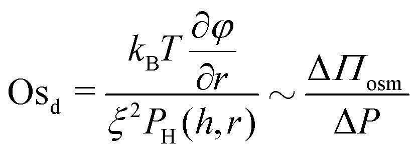
Similarly, we define a dynamic osmotic number, Osd that describes the relative importance of lateral osmotic stresses because of concentration gradients with respect to the viscous ones arising because of drainage:
 | (7) |
For concentrations close to the overlap concentration c*, as those employed in our study, it can be assumed that ξ ≈ RH.68 Although for monodisperse polymers differences in osmotic pressure ΔΠosm and thus osmotic stresses arise only because of concentration gradients in bulk, in solutions containing polydisperse polymers, like those studied here, differences in the molecular weight, ΔMw, also contribute to ΔΠosm. Therefore, as mentioned above for Osst, by changing the size (or molecular weight) distribution and the initial concentration (which will also affect ∂φ/∂r) we can tune the magnitude of the lateral osmotic stresses.
Using a virial expansion, the osmotic pressure of polymer solutions can be approximated as:69
 | (8) |
![[R with combining macron]](https://www.rsc.org/images/entities/i_char_0052_0304.gif) is the gas constant, and
is the gas constant, and  is an effective virial coefficient (ESI†). Eqn (8) can qualitatively describe the increase in the osmotic pressure that is expected for polymer solutions above c*.68 As mentioned above, when concentration differences Δc are present, these will result in osmotic pressure differences ΔΠosm. Eqn (8) indicates that the magnitude of the lateral osmotic stresses between a depleted and a concentrated region will be different for a given Δc when the initial concentration is close to c*. The calculated static and dynamic osmotic numbers can be found in the ESI.†
Finally, concentration gradients in bulk are expected to depend on the Péclet number:
 | (9) |
3 Materials and methods
3.1 Materials
Three different grades of polyisobutylene (PIB) were used in this study. Oppanol B10SFN, and B50SFN were provided by BASF (Ludwigshafen, Germany), and P500 was purchased from Polysciences Inc. (Warrington, USA). The weight-average molecular weight and the polydispersity index of each polymer as determined by Gel Permeation Chromatography is shown in Table 1 (average of two measurements). The full molecular weight distribution (ESI†) was determined using an Agilent GPC 1260 Iso at 35 °C with a refractive index and a UV-VIS (254 nm) detector. THF was used as a solvent.| Polymer (tradename) | Weight-average molecular weight, Mw (g mol−1) | Polydispersity index, PDI (−) | R H (nm) | R G (nm) | c* (wt%) |
|---|---|---|---|---|---|
| P500 | 1273 | 2.1 | 0.83 ± 0.06 | 1.1 | 62.2 |
| B10SFN | 57![[thin space (1/6-em)]](https://www.rsc.org/images/entities/char_2009.gif) 635 635 |
2.8 | 5.5 ± 0.1 | 7.2 | 9.7 |
| B50SFN | 327079 |
1.5 | 14.3 ± 0.2 | 17.2 | 3.7 |
The critical molecular weight for the onset of entanglements is Mc = 13100 g mol−1.70 All grades are stabiliser-free and IR spectroscopy showed no presence of heteroatoms. n-Hexadecane was purchased from Acros Organics and has a purity of 99%. Hexadecane is a good solvent for PIB, with a Flory interaction parameter χF in the range of 0.3–0.43.71 In the case of B10SFN, four different solutions were prepared, with concentrations of 1, 5, 10, and 15 wt%. The solutions of the B10SFN act as the reference case for which lateral osmotic stresses are negligible. The concentrations of the two other PIB grades were chosen so that the bulk viscosities of the prepared solutions are equal to the 10 wt% B10SFN solution. We were thus able to study the effect that the osmotic stresses have on drainage, while keeping the hydrodynamic conditions constant. All solutions were filtered with a 0.2 μm PTFE filter before usage.
For each polymer, the critical overlap concentrations was calculated following Graessley:72
 | (10) |
 , where b is the C–C bond length, C∞ is the characteristic ratio, and Mu the molecular weight of the repeating unit.73 For polyisobutylene b = 0.1505 nm,74 and C∞ = 6.7.75 Given the wide molecular weight distributions of the polymers in our study, c* was estimated using the average of the weight- and number-average molecular weights (ESI†). The values of c* shown in Table 1 can vary up to ∼20% depending on the choice of the Mw, given the broad PDI of the polymer. The calculated RG (Table 1) results in RG/RH ratios in the range of 0.75-0.8, as expected for linear polymers dissolved in good solvents.76
3.2 Methods
| Polymer (tradename) | Concentration wt% | Viscosity (mPa s) | Surface tension (mN m−1) |
|---|---|---|---|
| P500 | 52 | 19.8 ± 0.1 | 27.5 ± 0.1 |
| B10SFN | 1 | 3.5 ± 0.1 | 27.3 ± 0.1 |
| 5 | 7.7 ± 0.1 | 27.3 ± 0.1 | |
| 10 | 18.3 ± 0.2 | 27.4 ± 0.1 | |
| 15 | 37.7 ± 0.3 | 27.4 ± 0.1 | |
| B50SFN | 2.5 | 18.9 ± 0.5 | 27.4 ± 0.1 |
| n-Hexadecane | 0 | 3.1 ± 0.182,83 | 27.4 ± 0.1 |
 | ||
| Fig. 1 Experimental setup and experimental approach: (a) a thin liquid film is formed in the hole of the bikewheel (cross section shown). Upon application of an extra ΔP at the air-side results in liquid being pushed out through the side-channels. The presence of multiple side-channels allows the symmetric drainage of films of relatively high viscosities. (b) Interferometric images during the various thinning regimes. The coalescence time is defined as the interval between the onset of film expansion (t = t0) and film rupture (t = tc). (c) The expansion of the film and its thinning as a function of time. The definitions of the various regimes and times during a drainage experiment are also shown. (d) The coalescence times of solutions of medium Mw PIB B10SFN at four different concentrations as a function of pressure. Adapted from ref. 57. | ||
The pressure inside the chamber is controlled by an Elveflow MK3+ piezoelectric pressure control system which has a resolution of 1 Pa and a maximum pressure of 20 kPa. The response time was independently measured by coupling the control system to a Barathron 120AD differential pressure transducer, and was found to be O(10−2 s). The application of the desired pressure step was followed by an initial pressure overshoot (of a maximum relative magnitude of ∼20% for low ΔP) that settled after O(10−1 s). The control system is connected to the pressure chamber by rigid PTFE tubing with an inner diameter of 0.1 mm.
The film visualisation is done with a Nikon Eclipse FN1 fixed-stage upright microscope (to minimise vibrations) and a 10× long working distance objective with a numerical aperture of 0.30. The entire setup being mounted onto an active noise cancelling table. The film is monitored by a Hamamatsu ORCA-Flash4.0 CMOS camera. A monochromatic wavelength of 508 nm was used for imaging in reflection. A sequence of images is saved (with a maximum of 10 ms temporal resolution) and is then converted to thickness using the Sheludko equation:1
 | (11) |
The experimental procedure and an example of the resulting evolution of the radius and the thickness of a 5 wt% polymer film film are shown in Fig. 1c for a 50 Pa pressure drop. Initially a thick film is created and its equilibrium pressure is determined by applying a pressure equal to Pc,i at the gas phase. The equilibrium point can be easily determined by varying the pressure in steps of 1 Pa until the first interference fringes that appear when the thickness of the TLF is in the order of a few μm are stable. More information regarding the experimental method and the involved pressures can be found in ref. 57. Subsequently, the pressure inside the film is lowered using pressure drops, ΔP, in the range of 20 to 1000 Pa. When the pressure drop is applied, the film begins to drain at a constant speed. This corresponds to a constant approach velocity regime, where h ∼ (−t). At a thickness of O(102 nm) the hydrodynamic pressure inside the film builds up, causing its expansion. This initial thickness depends on the applied pressure step.89,90 The pressure balance in the thin film is given by eqn (2).
The onset of film's expansion (when the first interference fringes are observed) is identified as the beginning of drainage, t0 (Fig. 1b and c). In the drainage regime, h ∼ (−t0.5), in agreement to the integrated form of the Reynolds equation (eqn (1)) (Fig. 1c and ESI†). As these polymer films are thermodynamically unstable, the end of drainage is set by the rupture of the film (Fig. 1b and c). A similar definition of coalescence time has been used by Kannan et al.91 At least 5 measurements were done for each combination of ΔP and polymer concentration for the B10SFN solutions, while at least 3 measurements were done for the P500 and B50SFN solutions.
4 Results and discussion
The simplest observable from the DTFB experiments is the coalescence time as defined in Section 3.2.4 for a given applied pressure drop (and hence Ca). In this section we will discuss (i) how the imposed ΔP affects the dynamics of films of different concentrations when osmotic stresses are negligible, and (ii) the effect of the polymer molecular weight and (iii) molecular weight distribution on the magnitude of osmotic stresses and the resulting film dynamics.4.1 Drainage dynamics of polymer solution films
For this Mw, the same trend is observed for all concentrations. A change in the slope of the coalescence time is observed at a pressure of the same magnitude as the Laplace pressure due to the film's curvature in the bikewheel (2σ/R). This critical pressure marks the gradual transition from a regime where drainage is slow92 to a hydrodynamically-dominated regime in which the coalescence time is inversely proportional to the applied pressure drop.57 The differences between the coalescence times of the various solutions were found to be proportional to their bulk viscosity, as expected from eqn (1). More details on drainage, and specifically on the temporal evolution of the thickness, radius, and volume of the films for the employed range of Ca can be found in the ESI.†
Although the coalescence times of all solutions were proportional to the viscosity (within experimental accuracy), the microscopically observed behaviour was quite complex. The various patterns that were observed during drainage of the medium Mw solutions are shown in Fig. 2. The probability for asymmetric drainage accompanied by flow instabilities, as well as the type of the latter, depended non-trivially on polymer concentration and the applied Ca.
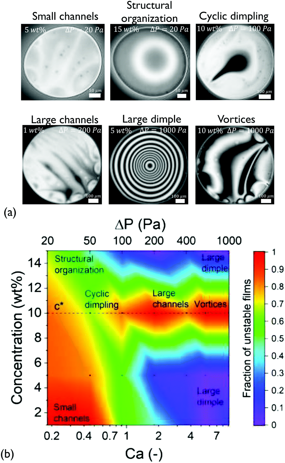 | ||
| Fig. 2 Thin film dynamics of the medium Mw solutions: (a) microinterferometric images of selected snapshots highlighting characteristic patterns. A variation of drainage type with polymer concentration and applied ΔP was observed. (b) State diagram describing the propensity of films of different concentrations to show asymmetric drainage. Films become distinctly unstable at c*. The black points correspond to conditions at which detailed experimental observations were performed. | ||
At low Ca, small thickness corrugations and dark spots were observed, in agreement with the results of Nikolov and Wasan18 on films containing nanoparticles. In the latter case, the occurrence of thickness fluctuations was observed in the regions in the film where particles are present. The thickness of the dark spots at low ΔP just before rupture is 30 ± 9 nm. The thickness of these dark domains did not depend on the RH of the polymer, with the films of P500 (with RH ≃ 1 nm) having similar minimum thickness values (ESI†). The critical thickness measured just before rupture is always located in such a dark spot, and can be predicted by simple rupture models that neglect osmotic effects.57 Therefore, this suggests that these regions contain no polymer molecules, in agreement with earlier results on nanoparticle-containing films.94
Interestingly, at the highest concentration some films showed thickness steps in the radial direction, observed as abrupt grayscale variations in the 15 wt% films at ΔP = 20 Pa (Fig. 2a). The obtained thickness profile (ESI†), suggests that a lateral organisation exists within the film. This effect, which has been predicted by Klapp et al.95 and reported for wetting films,96 has not been previously observed in freestanding films with deformable surfaces.
Effect of concentration. Upon increasing the applied pressure, the behaviour of the films depended significantly on concentration. The drainage could proceed either axisymmetrically, with the formation of a dimple at the centre of the film97 or asymmetrically, accompanied by dimple wash-outs which in certain cases were followed by the dimple reforming,41 the formation of channels of higher thickness,37 and even the formation of vortices close to the edge of the film (Fig. 2a). The observed drainage modes depend non-trivially on the concentration of the dissolved polymer and the applied Ca. The cause of these instabilities are lateral osmotic stresses that will be discussed further below.
Because of the stochastic character of the asymmetric drainage, we plot the fraction of films that were unstable (i.e. not showing an axisymmetric dimple) as a function of Ca in a state diagram (Fig. 2b). In general, capillarity will tend to stabilise the film's shape. The probability for symmetric drainage hence increases with Ca, following a normal cumulative distribution function (ESI†). The exact prediction of the conditions at which instabilities occur would require a linear stability analysis, similar to that conducted for instabilities caused by Marangoni stresses.98,99 Organising the observed instabilities in a state diagram can provide some insight on the involved processes. For c < c* (1 and 5 wt%) the behaviour of the films was quite similar. Increasing Ca results in a gradual stabilisation of the dimple and a transition from slightly asymmetric drainage observed at low Ca to a fully axisymmetric drainage. The origin of the unstable regime at low Ca is related to the weak stabilising effect of capillary forces. At this regime small thickness corrugations are observed despite the relatively small expected magnitude of lateral osmotic stresses.
The dimple size increases with the applied Ca and the thickness at the centre scales as hcent ∝ Ca (ESI†). The linear dependence is slightly lower than the 3/2 exponent predicted by simulations,100,101 which could be attributed to the complexity of the phenomena taking place during the drainage of the polymer solutions and to the standard deviation of the measurements. The same gradual transition to the dimpled configuration was also observed for the 15 wt% film, with the exception of the lateral structural organisation at low Ca that was described above. Apart from the stabilising effect of Ca, the re-stabilisation of the film's dimpled shape with increasing ΔP is in agreement with the Pe-dependent transport of polymer molecules. As discussed in Section 2, when the thinning rate of the film is high, the transport of the polymer molecules becomes convection-dominated. Such large drag forces are known to equalise the relative velocities of the polymer and solvent,63 thus minimising any concentration and osmotic pressure differences.
Propensity for instabilities close to c*. The drainage sequences of the films with a concentration close to the critical concentration (c = 10 wt% ≃ c*) show highly unstable, asymmetric patterns for all values of Ca (Fig. 2b and ESI†). These instabilities actually become more pronounced with Ca, changing gradually from small channels, over cyclic dimples, to large channels and vortices.
This propensity for instabilities close to c* is an indication that lateral osmotic stresses develop in the films. At c*, as we move from the dilute to the semi-dilute regime, polymer–polymer interactions result in a change in the concentration dependence of osmotic pressure from a linear to a non-linear one.64,68 Hence, when the initial concentration is close to c*, as in the case of the 10 wt% solution, an induced concentration difference results in a strong pressure imbalance between the concentrated and the depleted region, with the polymer molecules interacting only in the former. Thus, the resulting unequal osmotic stresses will cause an inhomogeneous bulk stress distribution in the film, destabilising the outflow of the liquid.
The occurrence of these instabilities did not have a significant effect on the coalescence time (within the experimental limits of our technique). However, the volume of the film just before rupture was more strongly affected (ESI†). The 10 wt% solution, which is the most prone to asymmetric drainage, had the lowest estimated volume at rupture. This is an indication that the instabilities mentioned above have a strong effect on the liquid entrained inside the film. The dimple wash-outs and the formation of channels can be expected to accelerate the outflow of liquid.102 On the other hand, the overall enhanced viscous dissipation in the films due to the complex flow may slow down drainage globally. The net effect on coalescence time is still limited.
Characteristic timescale of instabilities. To prove that lateral osmotic stresses cause the instabilities, the characteristic timescales of the latter were determined from the time evolution of the thickness fluctuations, as in Fig. 3a. The local thinning velocity is obtained by differentiation dhcent/dt (Fig. 3b). The strong thickness peaks are caused by the dimple wash-out events, while the small peaks are caused by smaller scale instabilities, such as channels (Fig. 3c). The period for all instabilities, Tf, is taken to be equal to the time between two consecutive local minima, which correspond to the onset and end of each instability, respectively. Fig. 4 shows that Tf for different concentrations collapse onto a master curve and the determining variable is Osd, as defined in eqn (7). As the actual concentration difference in the film is unknown, we assumed that Δc ∼ c and calculated the expected ΔΠosm from eqn (8).
 | ||
| Fig. 3 Characteristic timescale of instabilities of the medium Mw solutions: (a) The drainage curve of a 5 wt% solution at ΔP = 100 Pa. (b) The corresponding thinning velocity. The temporal evolution of the two instabilities is shown with numbers. (c) Microinterferometry images of the same film, showing two instabilities, namely cyclic dimple formation and channel relaxation. The numbers of each image correspond to distinct times of the thinning velocity curve shown above. | ||
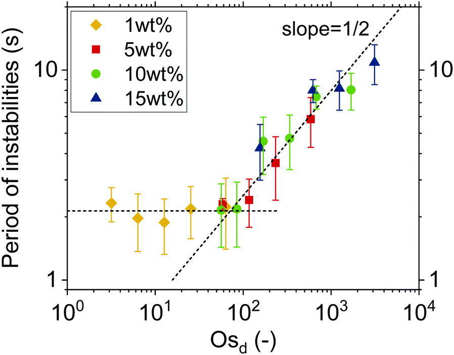 | ||
| Fig. 4 Dynamic Osd scaling: a master-curve is obtained for all concentrations of the medium Mw polymer solutions when plotting the characteristic timescale of the instabilities versus Osd. The two regimes are related to differences in the magnitude of Δc. | ||
Fig. 4 shows how the period of fluctuations is constant for low Osd and then increases with  . This can be rationalized by considering the relative magnitudes of hydrodynamic (ΔP) and osmotic pressure differences (ΔΠosm). We can assume that ΔP ∝ Δc, as in ref. 98. Concerning ΔΠosm, for small values of Δc, the second order term in eqn (8) can be neglected and the differences in osmotic pressure are also simply proportional to the applied pressure drop. As both ΔP and ΔΠosm are proportional to the applied pressure drop, Tf is constant. In contrast, for higher Δc, the c2 term in eqn (8) can no longer be neglected, and the relation between ΔΠosm and ΔP becomes non-linear. A
 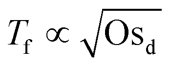 dependence, indicative of the occurrence of lateral osmotic forces, is observed experimentally over the experimentally accessible range in Fig. 4. For very high Δc, at which the the c2 term in eqn (8) becomes dominant, one would expect that Tf becomes proportional to Osd. The period of instabilities of the low Mw polymer solution (see ESI†) studied at c = 52 wt%, indicates that a gradual transition to a linear dependency might indeed occur for higher values of Osd.
Concluding, there are so far three different observations that support the argument that the dynamics of the polymer solution films are controlled by osmotic effects. First, the long coalescence times of O(100–102 s), which are observed despite the absence of surface stresses. Second, the occurrence of strong instabilities during the drainage of films, in particular for those solutions with concentrations close to c*. Finally, the fact that the time scale of the instabilities, as characterized by Tf, is controlled by Osd (Fig. 4). It can be noted that the procedure of determining the period of the instabilities could potentially be applied to surfactant micellar-containing foam films as well, thus enabling the separation of the osmotic effects from other contributions like Marangoni103 or even viscoelastic stresses.104
Despite the existence of osmotic stresses, it is evident that increasing just the concentration of the polymer in the solution is not a powerful method to exploit such effects. In the investigated concentration range, the coalescence times of all solutions were found to be proportional to the viscosity (Fig. 1d). Thus, the lateral dynamic osmotic stresses (Osd), and the increase in the normal Osst because of the increased concentration (calculated to be of O(10), ESI†) had only a small to negligible effect on the lifetime of the films. As it will be discussed in the next sections, changing the molecular weight and the molecular weight distribution of the dissolved polymer provide more effective means to further tune film dynamics.
4.2 Controlling the lifetime of thin films of polymer solutions
There are two ways by which osmotic stresses can affect the lifetime of the films. One way would be through Osst, which controls the static osmotic stresses that act normal to the film's surface and influence the disjoining pressure. The second way is more subtle, through Osd, which controls the magnitude of the osmotic stresses that act in the direction of flow, i.e. laterally.The coalescence times as a function of ΔP are shown in Fig. 5. As in Fig. 1d two distinct regimes are observed, separated at approximately 2σ/R. The significant differences in drainage times at low ΔP are directly related to the contribution of Osst to the disjoining pressure. The calculated Osst (eqn (6) and (8)) of the various solutions were found to be orders of magnitude different (ESI†). At ΔP = 50 Pa, the Osst of the low Mw can be estimated to be O(104), while for the medium Mw was of O(101), and for the high Mw was of O(10−1). As a result the coalescence times of the various solutions, differ at the low ΔP regime by almost an order of magnitude. Experimentally, a relation tc ∝ Mn−1/3 was observed.
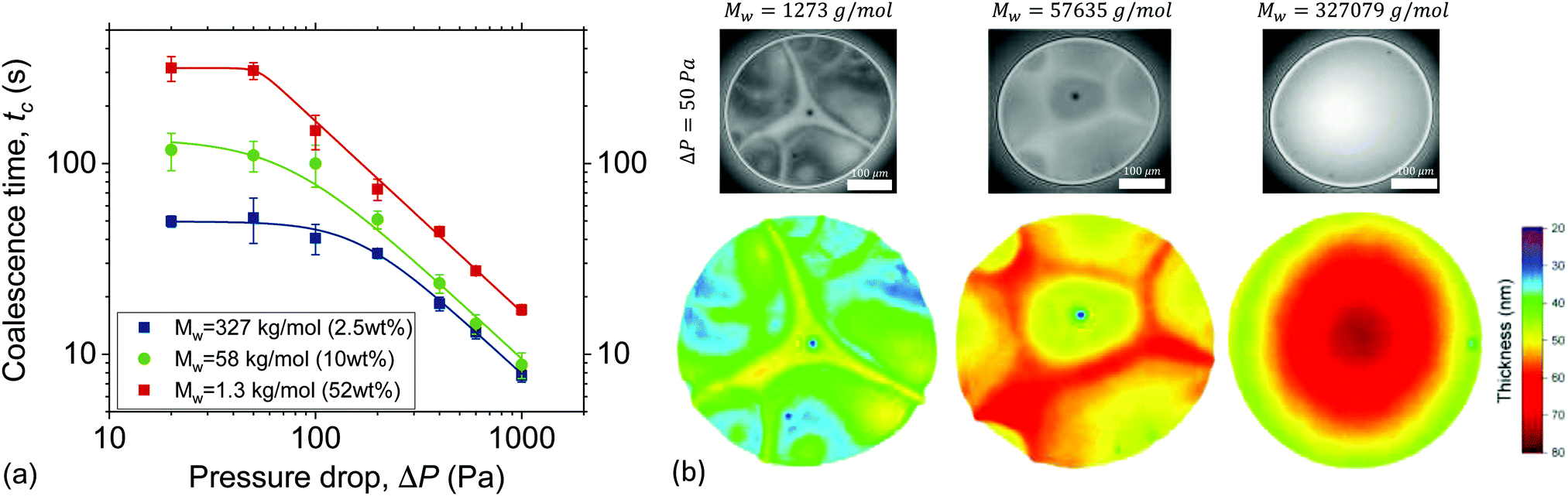 | ||
| Fig. 5 Effect of molecular weight on the coalescence time and drainage dynamics for equal viscosity solutions: (a) the coalescence times for different Mw as a function of ΔP. (b) Microinterferometry images of films of the same solutions just before rupture for ΔP = 50 Pa. The corresponding 3D thickness maps are shown below. The average thickness increases with Mw, while the radius of the film remains constant. | ||
This increased stability with reducing the size of the confined species has also been reported for micelles, nanoparticles26 and polyelectrolytes.28 However, it is usually observed as an increase in the amplitude of the structural oscillatory forces. The magnitude of the Osst might depend on the polydispersity18,26,29,30,32,39,40,105 and on the deformability of the confined polymer.27,33 However, studying these effects would require (i) the addition of polymers of the same Mn and different PDI, or (ii) the addition of polymers of the same Mn but different persistence lengths, and are thus beyond the scope of this study.
The contribution of static osmotic stresses can be inferred from the interferometry images of the films and their corresponding 3D thickness maps (Fig. 5b). The average thickness at rupture is found to differ, as expected based eqn (2).89 According to the 3D thickness maps, the average thickness at rupture of the films at ΔP = 50 Pa increases with Mw. This means that the static osmotic contribution is higher for the polymer with the smallest Mw, as it is able to counteract the attractive vdW disjoining pressure down to thicknesses of ∼30 nm. In contrast, the 57.6 kg mol−1 and the 327.1 kg mol−1 polymer films rupture when their average thickness is ∼50 nm and ∼60 nm, respectively. The absence of pronounced osmotic effects in the case of the highest Mw polymer resulted also in the complete absence of thickness corrugations. The differences in coalescence times reduces as ΔP increases (Fig. 5a). Previous studies with a bubble-probe AFM on air bubbles separated by polyelectrolyte-containing aqueous films also report an attenuation of the structural forces as hydrodynamics become dominant.28,29
As mentioned above, the films of the highest Mw showed no thickness corrugations and a much lower amount of dark spots (Fig. 5b), indicating that osmotic contributions are much smaller than the Laplace pressures. Interestingly, these films also showed a very small dimple or no dimple at all even at the highest applied ΔP (ESI†). The absence of a dimple at high nominal Ca is in general considered an indication of surface stress-free drainage.106,107 Films with Marangoni stresses can be planar, when axisymmetry in drainage is not maintained,10,16,108 but they always exhibit some thickness corrugations, which is not the case for the high Mw polymer solutions studied here. A comparison with simulations could provide definite conclusions on the magnitude of surface stresses in the draining films. Such polymer solutions with negligible lateral but finite normal osmotic stresses are nice model systems to study the effect of surface stresses on drainage, given that despite their relatively low viscosity they exhibit long coalescence times, orders of magnitude higher than those of stress-free films of e.g. pure water, which are of O(100–101) ms.93
Despite the complexity of film stabilisation using static osmotic pressure Osst, it is clear that for a given viscosity, monodisperse, low Mw polymers result in longer film lifetimes. This should be relevant for the design of multiphase materials containing non-adsorbing species, such as polyelectrolyte foams109 and polymer-containing emulsions.47 The higher stability of films containing species of small size is relevant for a wide range of (typically relevant) Ca numbers (Fig. 5a).
:10 v/v% ratio. As previously, the surface tension and bulk viscosity of the reference medium Mw solution and its bimodal solution are also made to be equal. The addition of such a small fraction of the low Mw polymer ensures that the normal static osmotic contribution does not vary a lot and hence any change in film dynamics is solely related to lateral dynamic effects. The experimentally obtained coalescence times of the bimodal solutions are shown together with the mono-component medium Mw polymer solution for a wide range of ΔP in Fig. 6a. As expected the coalescence times of the two solutions at low ΔP are the equal. This confirms that the addition of the low Mw polymer did not affect the Osst, which could be explained by the partition of smaller molecules within the excluded volume of larger ones in the film.28
 | ||
| Fig. 6 Effect of the molecular weight distribution on the coalescence times and drainage dynamics: (a) the coalescence times as a function of ΔP for two polymer films with different PDI. (b) Microinterferometry image of the bimodal film just before rupture at ΔP = 50 Pa. (c) The corresponding 3D thickness map. (d) The evolution of “dimple recoil”. The dimple moves towards the Plateau border until t = 32 s and then moves back towards the film's center. | ||
However, as of ΔP ≥ 400 Pa the solutions with the bimodal Mw distribution started showing significantly slower coalescence, which for the highest pressure steps applied were approximately double the tc of the pure solution. For these dynamics effects to occur, Pe should be relatively high to induce concentration differences and overcome bulk diffusion. The Pe number in our experiments can be estimated from eqn (9) using our experimental data for the film expansion rate and the radius,49 and a diffusion constant of 10.4 μm2 s−1 obtained by DLS for the medium Mw polymer. A Pe number of O(102–103) was calculated for ΔP ≥ 400 Pa. Apart from the larger ΔMw that can be attained if bimodal solutions exhibit concentration gradients, the dynamic stabilisation could also be facilitated by the fact that larger molecules experience a stronger drag force during drainage, which could potentially result in a more pronounced depletion from the film.29,110 Another estimate can be done regarding the magnitude of the concentration differences inside the film. Assuming that thickness corrugations will develop when ΔΠosm ∼ 2σ/R,37 a Δc ∼ 10% can be estimated from eqn (8) for the solution of the medium Mw polymer (ESI†).
The addition of the small amount of low Mw fraction resulted in an intensification of the flow instabilities. Vortices were observed even at a very low ΔP (Fig. 6b) and their occurrence strengthened with applied pressure. Moreover another flow phenomenon was observed, which has been previously termed as “dimple recoil”20 (Fig. 6c and Movie). At one point during drainage the dimple became unstable and moved towards the Plateau border (t = 29 s). Then, after approximately a few seconds the dimple started recoiling and restabilised at the film's centre. This effect was observed only at ΔP = 100 Pa ≃ 2σ/R. The occurrence of this instability only at this specific ΔP is probably related to the fact that at Ca ≃ 1 lateral osmotic stresses might locally be strong enough to destabilise the dimple, without however causing its complete collapse before hydrodynamics restabilise the flow. A similar “dimple recoil” was also recently observed in films of worm-like micelles and was attributed to bulk elasticity.20 However, strong structural forces are known to develop in films with worm-like micelles,25 which means that these systems also have a potential for exhibiting dynamic osmotic effects. Therefore, the origin of this effect might not necessarily be the elasticity of the film.
Overall, the polydisperisty in the Mw of the dissolved polymer had a strong effect on the observed film dynamics (Fig. 7a). In the state diagram of Fig. 7b we plot the fraction of unstable films as a function of the polydisperity index of the dissolved polymer for different employed Ca numbers. The three polymers of this study are considered together with the bimodal mixture, which is independently reported on top of the polydispersity axis. It is clear that low polydispersities favour symmetric drainage and the formation of a stable dimple. In contrast, the solutions of the more polydisperse polymers exhibited mostly asymmetric drainage. For the bimodal solution, the occurrence of large channels, vortices, and dimple recoils resulted in liquid recirculation within the films, doubling their lifetime.
 | ||
| Fig. 7 Thin film dynamics influenced by dynamic osmotic stresses: (a) microinterferometric images of polymer films of different PDIs. (b) State diagram describing the propensity for asymmetric drainage as a function of Ca and ΔP for films containing polymer of different PDIs. The black dots indicate the experimentally measured points. The bimodal mixture is separately shown at the top of the y-axis. | ||
The increase in the lifetime of films containing polymer mixtures takes place at relatively high Ca numbers and, as such, may have gone unnoticed in earlier work. The occurrence of these dynamic osmotic stresses could have significant implications for various technological applications. For example, it is common industrial practice in lubricant technology to mix different lubricant grades to attain a certain desired viscosity.46 However, both lubricants and fuels typically contain polymer additives as viscosity modifiers.111 Furthermore, wide polymer molecular weight distributions are also expected to develop over time in mechanosensitive formulations.112 Our results suggest that such multicomponent systems are more prone to foaming, the latter being undesirable in lubricants46 and fuels.113
5 Conclusions
The dynamics of freestanding liquid films containing dilute and semi dilute polymer solutions were studied using a dynamic thin film balance. The effect of polymer concentration, molecular weight, and molecular weight polydispersity were examined over a wide range of capillary numbers. The viscosity of the solutions was kept constant, while the Mw and the concentration of the polymers was changed. The thinning dynamics were found to be influenced by the static osmotic pressure that is exerted by the confined polymer molecules, in line with earlier work.26However, osmotic stresses acted not only normal to the film surface a but also laterally. At sufficiently high drainage rates, the flow induced concentration differences give rise to osmotic stresses. The drainage of the films was found to proceed either symmetrically, with the characteristic dimple formation97 or asymmetrically, with thickness corrugations, channels, vortices and other flow instabilities. The type of drainage depends non-trivially on the applied pressure drop, the concentration, the molecular weight and the polydispersity of the polymer. The characteristic timescale for the evolution of the observed instabilities was found to scale with a dynamic osmotic number, which relates the magnitude of lateral osmotic stresses to the hydrodynamic ones.
It was shown that at constant bulk viscosity, the films containing the polymer with the lowest Mw were the most stable, exhibiting coalescence times as high as 300 s despite the absence of surface stresses. In contrast, the high Mw polymer films drained symmetrically and their behaviour was in line with the thinning of films with stress-free surfaces.106,107 Mixing polymer grades with different Mw resulted in an intensification of the lateral osmotic pressure gradients that doubled the coalescence time in the high Ca regime. Channels, vortices, cyclic dimples and dimple recoils were observed, showing the richness of the dynamics of such films consisting of “simple” polymer solutions. These results provide new insights in the stabilisation mechanisms of films draining at realistically high Ca. The results presented contribute to a better understanding and potential optimisation of the formulation products, such as foams, emulsions, and lubricants, in which polymers are typically added as viscosity modifiers.
Conflicts of interest
There are no conflicts to declare.Acknowledgements
The authors would like to thank the ETH Energy Science Center Partnership with Shell for the financial support and A. Napoli and S. Arabin (Huntsman Advanced Materials GmbH) for conducting the GPC measurements. The help of Dr K. “Cannonball” Feldman (ETH Zurich) with the DLS measurements is also gratefully acknowledged.References
- A. Sheludko, Adv. Colloid Interface Sci., 1967, 1, 391–464 CrossRef CAS.
- N. Denkov, S. Tcholakova, K. Golemanov, K. Ananthapadmanabhan and A. Lips, Phys. Rev. Lett., 2008, 100, 138301 CrossRef CAS PubMed.
- J. M. Frostad, D. Tammaro, L. Santollani, S. B. de Araujo and G. G. Fuller, Soft Matter, 2016, 12, 9266–9279 RSC.
- J. Bibette, D. C. Morse, T. Witten and D. Weitz, Phys. Rev. Lett., 1992, 69, 2439 CrossRef CAS PubMed.
- U. Sundararaj and C. Macosko, Macromolecules, 1995, 28, 2647–2657 CrossRef CAS.
- B. Scheid, S. Dorbolo, L. R. Arriaga and E. Rio, Phys. Rev. Lett., 2012, 109, 264502 CrossRef PubMed.
- Y. Vitry, S. Dorbolo, J. Vermant and B. Scheid, Advances in colloid and interface science, 2019 Search PubMed.
- I. B. Ivanov, Pure Appl. Chem., 1980, 52, 1241–1262 CAS.
- N. Jaensson and J. Vermant, Curr. Opin. Colloid Interface Sci., 2018, 37, 136–150 CrossRef CAS.
- E. Chatzigiannakis, N. Jaensson and J. Vermant, Curr. Opin. Colloid Interface Sci., 2021, 101441 CrossRef CAS.
- V. Bergeron, J. Phys.: Condens. Matter, 1999, 11, R215 CrossRef CAS.
- L. G. Cascão Pereira, C. Johansson, C. J. Radke and H. W. Blanch, Langmuir, 2003, 19, 7503–7513 CrossRef.
- D. Langevin, Adv. Colloid Interface Sci., 2000, 88, 209–222 CrossRef CAS PubMed.
- E. Hermans, M. S. Bhamla, P. Kao, G. G. Fuller and J. Vermant, Soft Matter, 2015, 11, 8048–8057 RSC.
- K. D. Danov, D. S. Valkovska and I. B. Ivanov, J. Colloid Interface Sci., 1999, 211, 291–303 CrossRef CAS PubMed.
- S. I. Karakashev, D. S. Ivanova, Z. K. Angarska, E. D. Manev, R. Tsekov, B. Radoev, R. Slavchov and A. V. Nguyen, Colloids Surf., A, 2010, 365, 122–136 CrossRef CAS.
- S. Narayan, A. E. Metaxa, R. Bachnak, T. Neumiller and C. S. Dutcher, Curr. Opin. Colloid Interface Sci., 2020, 50, 101385 CrossRef CAS.
- A. Nikolov and D. T. Wasan, Langmuir, 1992, 8, 2985–2994 CrossRef CAS.
- R. R. Dagastine, G. B. Webber, R. Manica, G. W. Stevens, F. Grieser and D. Y. Chan, Langmuir, 2010, 26, 11921–11927 CrossRef CAS PubMed.
- V. Chandran Suja, A. Kannan, B. Kubicka, A. Hadidi and G. G. Fuller, Langmuir, 2020, 36, 11836–11844 CrossRef CAS PubMed.
- C. Mitrias, N. Jaensson, M. Hulsen and P. Anderson, Microfluid. Nanofluid., 2019, 23, 87 CrossRef.
- V. Bergeron, Langmuir, 1997, 13, 3474–3482 CrossRef CAS.
- N. Kristen and R. von Klitzing, Soft Matter, 2010, 6, 849–861 RSC.
- X. Chu, A. Nikolov and D. Wasan, J. Chem. Phys., 1995, 103, 6653–6661 CrossRef CAS.
- A. Espert, R. v. Klitzing, P. Poulin, A. Colin, R. Zana and D. Langevin, Langmuir, 1998, 14, 4251–4260 CrossRef CAS.
- D. Wasan, A. Nikolov and F. Aimetti, Adv. Colloid Interface Sci., 2004, 108, 187–195 CrossRef PubMed.
- N. C. Christov, K. D. Danov, Y. Zeng, P. A. Kralchevsky and R. von Klitzing, Langmuir, 2010, 26, 915–923 CrossRef CAS PubMed.
- C. Browne, R. F. Tabor, F. Grieser and R. R. Dagastine, J. Colloid Interface Sci., 2015, 451, 69–77 CrossRef CAS PubMed.
- C. Browne, R. F. Tabor, F. Grieser and R. R. Dagastine, J. Colloid Interface Sci., 2015, 449, 236–245 CrossRef CAS PubMed.
- A. Nikolov and D. Wasan, Colloids Surf., A, 1997, 128, 243–253 CrossRef CAS.
- W. Xu, A. Nikolov and D. Wasan, AIChE J., 1997, 43, 3215–3222 CrossRef CAS.
- D. Wasan and A. Nikolov, Curr. Opin. Colloid Interface Sci., 2008, 13, 128–133 CrossRef CAS.
- C. Uzum, S. Christau and R. von Klitzing, Macromolecules, 2011, 44, 7782–7791 CrossRef.
- S. Schon, M. Richter, M. Witt and R. v. Klitzing, Langmuir, 2018, 34, 11526–11533 CrossRef PubMed.
- Y. Zeng and R. von Klitzing, Soft Matter, 2011, 7, 5329–5338 RSC.
- R. F. Tabor, H. Lockie, D. Y. Chan, F. Grieser, I. Grillo, K. J. Mutch and R. R. Dagastine, Soft Matter, 2011, 7, 11334–11344 RSC.
- O. Velev, T. Gurkov, I. Ivanov and R. Borwankar, Phys. Rev. Lett., 1995, 75, 264 CrossRef CAS PubMed.
- S. A. Chen, L. Y. Clasohm, R. G. Horn and S. L. Carnie, Langmuir, 2015, 31, 9582–9596 CrossRef CAS PubMed.
- S. Biggs, Phys. Chem. Chem. Phys., 2010, 12, 4172–4177 RSC.
- M. Piech and J. Y. Walz, J. Colloid Interface Sci., 2002, 253, 117–129 CrossRef CAS PubMed.
- O. Velev, K. Danov and I. Ivanov, J. Dispersion Sci. Andtechnol., 1997, 18, 625–645 CrossRef CAS.
- O. D. Velev, T. D. Gurkov and R. P. Borwankar, J. Colloid Interface Sci., 1993, 159, 497 CrossRef CAS.
- K. D. Danov, T. D. Gurkov, T. Dimitrova, I. B. Ivanov and D. Smith, J. Colloid Interface Sci., 1997, 188, 313–324 CrossRef CAS.
- X. Zhang, R. Manica, Q. Liu and Z. Xu, Langmuir, 2021, 37, 4121–4128 CrossRef CAS PubMed.
- A. Martini, U. S. Ramasamy and M. Len, Tribol. Lett., 2018, 66, 58 CrossRef.
- V. C. Suja, A. Kar, W. Cates, S. Remmert, P. Savage and G. Fuller, Proc. Natl. Acad. Sci. U. S. A., 2018, 115, 7919–7924 CrossRef CAS PubMed.
- A. Meller and J. Stavans, Langmuir, 1996, 12, 301–304 CrossRef CAS.
- C. I. Browne, PhD thesis, University of Melbourne, 2016.
- E. Chatzigiannakis, P. Veenstra, D. ten Bosch and J. Vermant, Soft Matter, 2020, 16, 9410–9422 RSC.
- O. Reynolds, Philos. Trans. R. Soc. London, 1886, 157–234 Search PubMed.
- D. Y. Chan, E. Klaseboer and R. Manica, Soft Matter, 2011, 7, 2235–2264 RSC.
- D. S. Valkovska, K. D. Danov and I. B. Ivanov, Adv. Colloid Interface Sci., 2002, 96, 101–129 CrossRef CAS PubMed.
- D. Y. Chan, E. Klaseboer and R. Manica, Soft Matter, 2010, 6, 1809–1815 RSC.
- A. S. Hsu, A. Roy and L. G. Leal, J. Rheol., 2008, 52, 1291–1310 CrossRef CAS.
- V. V. Yaminsky, S. Ohnishi, E. A. Vogler and R. G. Horn, Langmuir, 2010, 26, 8061–8074 CrossRef CAS PubMed.
- S. Karakashev, Colloids Surf., A, 2010, 372, 151–154 CrossRef CAS.
- E. Chatzigiannakis and J. Vermant, Phys. Rev. Lett., 2020, 125, 158001 CrossRef CAS PubMed.
- J. C. Eriksson and B. V. Toshev, Colloids Surf., 1982, 5, 241–264 CrossRef CAS.
- F. Brochard and P. De Gennes, Macromolecules, 1977, 10, 1157–1161 CrossRef CAS.
- M. Cromer, G. H. Fredrickson and L. Gary Leal, J. Rheol., 2017, 61, 711–730 CrossRef CAS.
- A. Groisman and V. Steinberg, Nature, 2000, 405, 53–55 CrossRef CAS PubMed.
- L. Quinzani, G. McKinley, R. Brown and R. Armstrong, J. Rheol., 1990, 34, 705–748 CrossRef.
- S. T. Milner, Phys. Rev. E: Stat., Nonlinear, Soft Matter Phys., 1993, 48, 3674 CrossRef CAS PubMed.
- M. Rubinstein, R. H. Colbyet al., Polymer physics, Oxford University Press, New York, 2003, vol. 23 Search PubMed.
- G. H. Fredrickson, A. J. Liu and F. S. Bates, Macromolecules, 1994, 27, 2503–2511 CrossRef CAS.
- J. W. van Egmond and G. G. Fuller, Macromolecules, 1993, 26, 7182–7188 CrossRef CAS.
- A. Trokhymchuk, D. Henderson, A. Nikolov and D. T. Wasan, Langmuir, 2001, 17, 4940–4947 CrossRef CAS.
- R. H. Colby, Rheol. Acta, 2010, 49, 425–442 CrossRef CAS.
- C. M. Kok and A. Rudin, J. Appl. Polym. Sci., 1981, 26, 3575–3582 CrossRef CAS.
- L. Fetters, D. Lohse and R. Colby, Physical properties of polymers handbook, Springer, 2007, pp. 447–454 Search PubMed.
- P. Bataille and D. Patterson, J. Polym. Sci., Part A: Gen. Pap., 1963, 1, 3265–3275 CrossRef CAS.
- W. W. Graessley, Polymer, 1980, 21, 258–262 CrossRef CAS.
- C. Clasen, J. Plog, W.-M. Kulicke, M. Owens, C. Macosko, L. Scriven, M. Verani and G. H. McKinley, J. Rheol., 2006, 50, 849–881 CrossRef CAS.
- L. Bartell and R. Bonham, J. Chem. Phys., 1960, 32, 824–826 CrossRef CAS.
- U. Suter, E. Saiz and P. J. Flory, Macromolecules, 1983, 16, 1317–1328 CrossRef CAS.
- C. M. Kok and A. Rudin, Makromol. Chem., Rapid Commun., 1981, 2, 655–659 CrossRef CAS.
- L. Fetters, N. Hadjichristidis, J. Lindner and J. Mays, J. Phys. Chem. Ref. Data, 1994, 23, 619–640 CrossRef CAS.
- M. Kaszuba, D. McKnight, M. T. Connah, F. K. McNeil-Watson and U. Nobbmann, J. Nanopart. Res., 2008, 10, 823–829 CrossRef CAS.
- P. G. De Gennes, Macromolecules, 1981, 14, 1637–1644 CrossRef CAS.
- H. Edwards, J. Appl. Polym. Sci., 1968, 12, 2213–2224 CrossRef CAS.
- S. Wu, J. Colloid Interface Sci., 1969, 31, 153–161 CrossRef CAS.
- B. Coursey and E. L. Heric, J. Chem. Eng. Data, 1969, 14, 426–430 CrossRef CAS.
- G. P. Dubey and M. Sharma, J. Chem. Eng. Data, 2008, 53, 1032–1038 CrossRef CAS.
- L. C. Pereira, C. Johansson, H. Blanch and C. Radke, Colloids Surf., A, 2001, 186, 103–111 CrossRef.
- P. J. Beltramo, R. Van Hooghten and J. Vermant, Soft Matter, 2016, 12, 4324–4331 RSC.
- T. M. Aminabhavi and G. Bindu, J. Chem. Eng. Data, 1994, 39, 529–534 CrossRef CAS.
- Y. Zhang, S. Yilixiati, C. Pearsall and V. Sharma, ACS Nano, 2016, 10, 4678–4683 CrossRef CAS PubMed.
- P. J. Beltramo and J. Vermant, ACS Omega, 2016, 1, 363–370 CrossRef CAS PubMed.
- A. Chesters, Chem. Eng. Res. Des., 1991, 69, 259–270 CAS.
- F. Baldessari and L. G. Leal, Phys. Fluids, 2006, 18, 013602 CrossRef.
- A. Kannan, I. C. Shieh, D. L. Leiske and G. G. Fuller, Langmuir, 2018, 34, 630–638 CrossRef CAS PubMed.
- H. Yang, C. C. Park, Y. T. Hu and L. G. Leal, Phys. Fluids, 2001, 13, 1087–1106 CrossRef CAS.
- B. Liu, R. Manica, Q. Liu, E. Klaseboer, Z. Xu and G. Xie, Phys. Rev. Lett., 2019, 122, 194501 CrossRef CAS PubMed.
- G. N. Sethumadhavan, A. D. Nikolov and D. T. Wasan, J. Colloid Interface Sci., 2001, 240, 105–112 CrossRef CAS PubMed.
- S. H. Klapp, Y. Zeng, D. Qu and R. von Klitzing, Phys. Rev. Lett., 2008, 100, 118303 CrossRef PubMed.
- A. Chengara, A. D. Nikolov, D. T. Wasan, A. Trokhymchuk and D. Henderson, J. Colloid Interface Sci., 2004, 280, 192–201 CrossRef CAS PubMed.
- J. L. Joye, G. J. Hirasaki and C. A. Miller, Langmuir, 1992, 8, 3083–3092 CrossRef CAS.
- J.-L. Joye, G. J. Hirasaki and C. A. Miller, Langmuir, 1994, 10, 3174–3179 CrossRef CAS.
- X. Shi, M. Rodrguez-Hakim, E. S. Shaqfeh and G. G. Fuller, J. Fluid Mech., 2021, 915, A45 CrossRef CAS.
- M. Nemer, X. Chen, D. Papadopoulos, J. Bławzdziewicz and M. Loewenberg, Phys. Rev. Lett., 2004, 92, 114501 CrossRef CAS PubMed.
- P. Janssen, P. Anderson, G. Peters and H. Meijer, J. Fluid Mech., 2006, 567, 65 CrossRef.
- D. Weaire, M. Vaz, P. Teixeira and M. Fortes, Soft Matter, 2007, 3, 47–57 RSC.
- J. Lee, A. Nikolov and D. Wasan, Langmuir, 2016, 32, 4837–4847 CrossRef CAS PubMed.
- V. Chandran Suja, A. Kannan, B. Kubicka, A. Hadidi and G. G. Fuller, Langmuir, 2020, 36, 11836–11844 CrossRef CAS PubMed.
- G. A. Pilkington and W. H. Briscoe, Adv. Colloid Interface Sci., 2012, 179, 68–84 CrossRef PubMed.
- B. Dai and L. G. Leal, Phys. Fluids, 2008, 20, 040802 CrossRef.
- P. J. Janssen and P. D. Anderson, Macromol. Mater. Eng., 2011, 296, 238–248 CrossRef CAS.
- M. S. Bhamla, C. Chai, M. A. Alvarez-Valenzuela, J. Tajuelo and G. G. Fuller, PLoS One, 2017, 12, e0175753 CrossRef PubMed.
- A. Bureiko, A. Trybala, N. Kovalchuk and V. Starov, Adv. Colloid Interface Sci., 2015, 222, 670–677 CrossRef CAS PubMed.
- A. Darwiche, F. Ingremeau, Y. Amarouchene, A. Maali, I. Dufour and H. Kellay, Phys. Rev. E: Stat., Nonlinear, Soft Matter Phys., 2013, 87, 062601 CrossRef CAS PubMed.
- M. J. S. De Carvalho, P. R. Seidl, C. R. P. Belchior and J. R. Sodré, Tribol. Int., 2010, 43, 2298–2302 CrossRef.
- E. J. Soares, J. Nonnewton. Fluid Mech., 2020, 276, 104225 CrossRef CAS.
- A. Hilberer and S.-H. Chao, Encyclopedia of Polymer Science and Technology, Wiley Online Library, 2002 Search PubMed.
Footnote |
| † Electronic supplementary information (ESI) available. See DOI: 10.1039/d1sm00244a |
| This journal is © The Royal Society of Chemistry 2021 |