 Open Access Article
Creative Commons Attribution 3.0 Unported Licence
Leveraging autocatalytic reactions for chemical domain image classification†
Christopher E.
Arcadia
 a,
Amanda
Dombroski
b,
Kady
Oakley
b,
Shui Ling
Chen
b,
Hokchhay
Tann
a,
Christopher
Rose
a,
Eunsuk
Kim
a,
Amanda
Dombroski
b,
Kady
Oakley
b,
Shui Ling
Chen
b,
Hokchhay
Tann
a,
Christopher
Rose
a,
Eunsuk
Kim
 b,
Sherief
Reda
a,
Brenda M.
Rubenstein
b and
Jacob K.
Rosenstein
 *a
*a
aSchool of Engineering, Brown University, Providence, RI, USA. E-mail: jacob_rosenstein@brown.edu
bDepartment of Chemistry, Brown University, Providence, RI, USA
First published on 3rd March 2021
Abstract
Autocatalysis is fundamental to many biological processes, and kinetic models of autocatalytic reactions have mathematical forms similar to activation functions used in artificial neural networks. Inspired by these similarities, we use an autocatalytic reaction, the copper-catalyzed azide–alkyne cycloaddition, to perform digital image recognition tasks. Images are encoded in the concentration of a catalyst across an array of liquid samples, and the classification is performed with a sequence of automated fluid transfers. The outputs of the operations are monitored using UV-vis spectroscopy. The growing interest in molecular information storage suggests that methods for computing in chemistry will become increasingly important for querying and manipulating molecular memory.
Introduction
An autocatalytic reaction is one which is catalyzed by its own products. Such reactions can exhibit interesting behaviors such as self-sustaining growth and oscillation, and play important roles in living systems.1 Autocatalysis occurs in elements of cellular metabolism including glycolysis,2 mitosis,3 apoptosis,4 and DNA replication.5 Some have even posited that the origin of life may have had connections to the emergence of autocatalytic networks.6,7The dynamics of autocatalytic reactions share some features with modern machine learning algorithms, in which cascades of nonlinear operators are used to efficiently realize functions of arbitrary complexity.8 In theory, a network of autocatalytic reactions can be made analogous to an artificial neural network.9 Moreover, autocatalytic reactions have the beneficial property that their inputs and outputs can be represented by the same chemical species, potentially offering experimental scalability for deep feedforward networks.
The idea of chemical computing has a long history, inspired in part by the power, complexity, and energy efficiency of living systems.10,11 Recent advances in molecular information storage12–17 have brought these unconventional systems closer to reality and have renewed interest in chemical computing. Much of the research on molecular computing has focused on in vitro gene expression circuits18,19 and DNA strand–displacement reactions.20–22 While genomic networks have important experimental advantages, such as well-established catalytic enzymes, they represent a narrow slice of chemical space, and hybridization-based computation often suffers from slow reaction rates and temperature sensitivity. Outside of DNA, chemical computation has been demonstrated using oscillating reactions,23,24 metabolites,25 and phenols,26 and has been the subject of many theoretical studies. In silico chemical reaction networks27 have been designed to not only implement feedforward neural networks,28,29 but to both train and execute learned functions in simple perceptrons.30,31
We previously demonstrated a chemical perceptron which performs parallel computations on several datasets encoded in the co-existing concentrations of different chemical species.26 Using this system, we classified several handwritten digits from the MNIST database.32 However, this classifier was based on volumetric transfers of unreactive species, which amount to linear operations in the chemical domain. As a result, the final threshold operation had to be performed in silico.
Here, we combine automated fluid handling with an autocatalytic reaction to realize nonlinear operations in chemico. We encode digital images into catalyst concentrations, apply linear multiply-accumulate operations using volumetric liquid transfers, and perform winner-take-all (WTA) image classification with autocatalytic reactions. These demonstrations are a promising step in the nascent development of synthetic chemical computing systems.
Results and discussion
Kinetics of autocatalysis
A reaction in which one of the products speeds up further product formation is called autocatalytic. Consider the simplest autocatalytic reaction, which is given by:33 | (1) |
 | (2) |
 | (3) |
 | (4) |
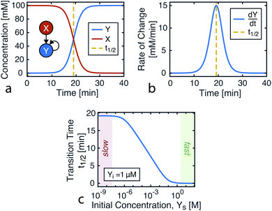 | ||
| Fig. 1 Kinetics of autocatalysis. (a) Reagent and autocatalytic product evolution over time for Xo = 100 mM, Yo = 1 μM, and k = 0.1 (eqn (4)). (b) Rate of product concentration change over time for the reaction simulated in a, showing the accelerated production typical of an autocatalytic process. (c) The time to transition as the input catalyst concentration (Yo) is varied about a constant: Yo = Yi + Ys with Yi = 1 μM, Xo = 100 mM, and k = 0.1. | ||
Relationship to artificial neural networks
An artificial neuron is a basic learning unit, inspired by biological neurons, which multiplies its inputs by a set of weights and transforms their sum through a nonlinear operator (the ‘activation function’).34 Interconnected sets of artificial neurons can perform classification tasks, among many other applications. In theory, the nonlinear kinetics of autocatalytic reactions could suggest chemical equivalents to electronic artificial neurons (Fig. 2). | ||
| Fig. 2 An artificial neuron implemented in the chemical domain through the programmable mixing and reacting of compounds from an autocatalytic process. | ||
For instance, the product evolution curve from eqn (4) is analogous to the popular logistic activation function.35 However, controlling this type of reaction through timing would be experimentally challenging. Previous theoretical work9 instead added a feedback path with a reverse reaction (Y back to X) with different kinetics. In this arrangement, the final product concentration ([Y]t→∞) was either a constant or zero, depending on whether the forward or reverse reactions were dominant. This network effectively produced a rectifying activation function.36 While simulations show this design could be robust against large concentration variations, it would be quite challenging to implement since it requires many complementary autocatalytic reactions with programmable reaction rates and limited cross-reactivity.
Taking into account experimental constraints, here we structure chemical computations around the time it takes for the product to evolve, using a single autocatalytic reaction as a nonlinear programmable time delay generator. In this model, the initial conditions are the input variable and the time to transition is the output (Fig. 1c). By using one reaction under varying initial conditions, data from a simple dilution ladder can provide sufficient calibration to design a computational network.
Time to transition
We define the time to transition, t1/2, as the time at which the product concentration, [Y], is halfway between its initial and final values: | (5) |
 | (6) |
For this reaction, the rate of increase in catalyst (d[Y]/dt) is greatest at tp = ln(Xo/Yo)/((Xo + Yo)k) which, assuming the initial concentration ratio is large (Xo/Yo ≫ 2) occurs roughly at the time to transition (tp ≈ t1/2). Using either of these time points as the output parameter, instead of the final concentration ([Y]t→∞), makes for more consistent computations since the final concentration tends to be more variable than the timing of catalysis (see Fig. 8c).
Copper-catalyzed Azide–Alkyne cycloaddition
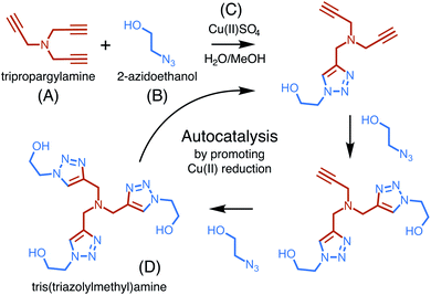
The copper-catalyzed reaction of an azide and an alkyne to form a 5-membered ring containing heteroatoms, known as a triazole, is one of the most well studied click reactions.37 These reactions have fast kinetics, are irreversible, use readily available starting material, occur under mild conditions, are high yield, and do not require purification.38 One such copper-catalyzed azide–alkyne cycloaddition (CuAAC) reaction was recently shown to exhibit particularly strong, autocatalytic rate enhancement.39 Carried out in a water–methanol solution containing a dissolved copper(II) salt, the reaction occurs through 1,3-cycloaddition and uses one equivalent of an alkyne, tripropargylamine, and three equivalents of an azide, 2-azidoethanol, to form a final product, tris(triazolylmethyl)amine, composed of three triazoles (Fig. 3).Rate enhancement was originally thought to be due to the formation of an intermediate which promotes the reduction of copper(II) to copper(I), a common catalyst.40 However, it has now been shown that the final product in complex with copper(I) is a more reactive catalyst for cycloaddition than copper(I) alone.41 The formation of tris(triazolylmethyl)amine increases copper(I) production and activity, thereby increasing its own formation and resulting in autocatalysis.
Monitoring reaction progress
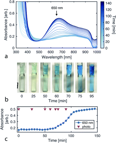
Since the CuAAC reaction involves multiple copper–ligand complexes which absorb visible light, we can quantitatively monitor reaction progress using UV-vis spectroscopy. Fig. 4a plots the reaction progression, with the broad absorption at 650 nm corresponding to the copper(II) complexes of triazolylmethylamine.39To initially validate the reaction, we carried out CuAAC reactions in cuvettes, allowing 290 mM 2-azidoethanol, 102 mM tripropargylamine, and 40 mM copper(II) sulfate to react while product formation was monitored using a UV-vis spectrophotometer (Varian Cary 50). The initial solution is transparent and colorless while the final solution containing the tris(triazolylmethyl)amine product has a blue tint (Fig. 4b).
For subsequent high-throughput experiments, we adapted the reaction to 384-well plates, using a UV-vis microplate reader (BioTek Synergy HTX) to track product formation.
Reaction parametrization
The CuAAC reaction time can be programmed by seeding the reaction with a small amount of tris(triazoloylmethyl)amine. The time to half completion (t1/2) is a function of the initial reagent concentrations ([A]t=0, [B]t=0, [C]t=0) and seed catalyst concentration ([D]t=0). By holding the starting reagent concentrations constant ([A]t=0 = 320.6 mM, [B]t=0 = 908.8 mM, and [C]t=0 = 126.5 mM), the catalyst concentration is made the only free variable.For the purposes of capturing the completion rate dependence on catalyst concentration, rather than developing a new system of differential equations to specifically model the CuAAC reaction, we can use eqn (6) as an intuitive template. By setting Xo = α and Yo = β + [D]t=0, we arrive at a parametric equation for the time to transition when only the catalyst concentration is varying:
 | (7) |
To obtain the catalyst ([D]t=0) for seeding the reaction, we pre-react a concentrated mixture ([A]t=0 = 1.308 M, [B]t=0 = 3.708 M, and [C]t=0 = 0.516 M) of reagents for 48 hours. For simplicity, we assume the reaction runs to completion, yielding a product concentration of 1.236 M, which is one third the concentration of the limiting reagent, the azide.
Transition time calibration
To model the constrained CuAAC, we performed a series of reactions with varying seed catalyst concentrations. Starting with concentrated pre-reacted solution (containing about 1.2 M of catalyst), we performed serial dilutions in 94% water and 6% methanol. Samples of 1 μL from each diluted catalyst solution were then transferred to a 384-well plate. In each well, 50 μL of starting reagent solution was added to initiate the reaction. Once the transfers were completed, the plate was placed in a UV-vis plate reader to obtain the absorbance traces shown in Fig. 5a.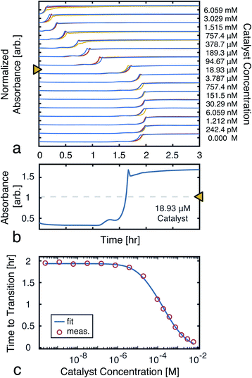 | ||
| Fig. 5 Time to transition calibration. (a) Absorbance (650 nm) traces used to monitor reaction progress as seed catalyst concentration was varied. The reactions were performed in triplicate to ensure the results were consistent. (b) A single trace from a ([D]t=0 = 18.93 μM), showing the mid-point line used to find the transition time. (c) Measured time to transitions for each tested catalyst concentration (averaged over the triplicates). A fit to eqn (7) is also shown. The model parameters were found, using nonlinear least-squares, to be: α = 2.81 mM, β = 14.2 μM, and k = 970 M−1 h−1. | ||
From the UV-vis traces, we extracted the time to transitions as the time points at which product absorbances were halfway between their initial and final values (Fig. 5b). Based on these curves, we fit a model of the transition time, which was in turn used for simulations and experiment planning (Fig. 5c).
Winner-take-all network
One algorithm suitable for reaction-based time delays is a winner-take-all (WTA) neural network.42 Such a network can be thought of as a race between potential classes, where the first class to reach a target state is deemed the winner. A diagram of a representative WTA network is shown in Fig. 8b, where each of the pooled outputs, yk, are associated with a different class. A comparison between the pools is used to determine the class of the input data (![[x with combining right harpoon above (vector)]](https://www.rsc.org/images/entities/i_char_0078_20d1.gif) ). Despite their relative simplicity, these networks can be designed to efficiently approximate any continuous function.43 Here, we set out to implement a chemical WTA network for image classification. An overview of the proposed computing framework is shown in Fig. 6.
). Despite their relative simplicity, these networks can be designed to efficiently approximate any continuous function.43 Here, we set out to implement a chemical WTA network for image classification. An overview of the proposed computing framework is shown in Fig. 6.
Encoding data in catalyst concentration
Digital images are represented chemically by the initial concentration of catalyst. Each pixel in a binary input image (![[x with combining right harpoon above (vector)]](https://www.rsc.org/images/entities/i_char_0078_20d1.gif) ) is assigned a position on a well plate, and an initial volume of solvent (Vs) is added to each of these wells. Then, for each white pixel (xn = 1), a small volume of pre-reacted solution (Vd), with a catalyst concentration Do, is added to its well. No catalyst is added to wells corresponding to black pixels (xn = 0). Thus the final catalyst concentration in data well n will be:
) is assigned a position on a well plate, and an initial volume of solvent (Vs) is added to each of these wells. Then, for each white pixel (xn = 1), a small volume of pre-reacted solution (Vd), with a catalyst concentration Do, is added to its well. No catalyst is added to wells corresponding to black pixels (xn = 0). Thus the final catalyst concentration in data well n will be: | (8) |
In-solution multiply and accumulate
The network inputs are mapped to class-specific pools through volumetric multiply-accumulate (MAC) operations.26 A small volume, vkn, is sampled from each of the n data wells and transferred to pool k. The amount taken from each well is set as vkn = wkn × Vu, where Vu is the maximum volume allowed to be transferred from a well and wkn ∈ [0, 1] is a tuning factor. By scaling the transfer volumes with weights trained on class k (![[w with combining right harpoon above (vector)]](https://www.rsc.org/images/entities/i_char_0077_20d1.gif) k), the summed output pool (yk) can be made to represent a single MAC operation on the catalyst-encoded input data (
k), the summed output pool (yk) can be made to represent a single MAC operation on the catalyst-encoded input data (![[d with combining right harpoon above (vector)]](https://www.rsc.org/images/entities/i_char_0064_20d1.gif) ). The resulting catalyst concentration in class k's pool is given by:
). The resulting catalyst concentration in class k's pool is given by: | (9) |
 This operation is repeated for each class, producing K output pools. At least Vs/Vu such pools could be made from a single data plate.
Autocatalytic activation and classification
Each of the MAC pools are composed solely of solvent and diluted catalyst, and as such only represent a linear combination of the inputs. To obtain the nonlinear response desired for classification, the autocatalytic reaction has to be initiated. To do so, a small volume, Vp, is transferred from each of the pools wells to their corresponding reaction wells, which were prefilled with Vr of starting reagent solution. At first, the seed catalyst concentration in reaction well k will be given by: | (10) |
![[thin space (1/6-em)]](https://www.rsc.org/images/entities/char_2009.gif) :
:![[thin space (1/6-em)]](https://www.rsc.org/images/entities/char_2009.gif) Vr roughly equal to 1
Vr roughly equal to 1![[thin space (1/6-em)]](https://www.rsc.org/images/entities/char_2009.gif) :
:![[thin space (1/6-em)]](https://www.rsc.org/images/entities/char_2009.gif) 50, then the time at which the catalyst concentration in well k reaches half its steady state value will be:
50, then the time at which the catalyst concentration in well k reaches half its steady state value will be:| τk = t1/2(rk) | (11) |
| τi < τj, ∀i ≠ j | (12) |
Experimental demonstration
Using the proposed approach, we built an autocatalytic WTA network for classifying binary images from the CalTech 101 16 × 16 Silhouettes dataset44 (Fig. S1 and S2†). The network was specifically designed to identify five (K = 5) of the more recognizable image classes: ‘starfish’, ‘kangaroo’, ‘llama’, ‘dragonfly’, and ‘ibis’ (68–86 images per class, shown in Fig. S3–S7†).Network weights were iteratively trained over 700 epochs, using a 70–30% train-test split (Fig. S8†). The training algorithm is described in the Methods, and the resulting weights are shown graphically in Fig. 7, alongside an example image from each class. Using these weights and the time to transition model from Fig. 5, we simulated the outputs of the network for one input image (Fig. 7c and d). Extending these simulations to the full train and test sets (398 images in total), the network was found to have a classification accuracy of 81.16% (Fig. S9†).
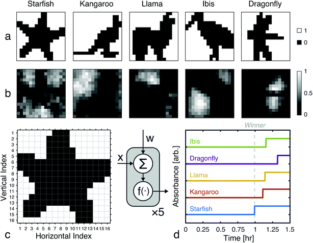 | ||
| Fig. 7 Network training and in silico simulation. (a) Example images from each of the considered classes. (b) Trained weights for each class. (c) The input, one of the starfish images from the test set, prior to being reshaped as a feature vector. (d) Simulation results obtained using the weights shown in (b), the image from (c), and the time to transition model from Fig. 5c. | ||
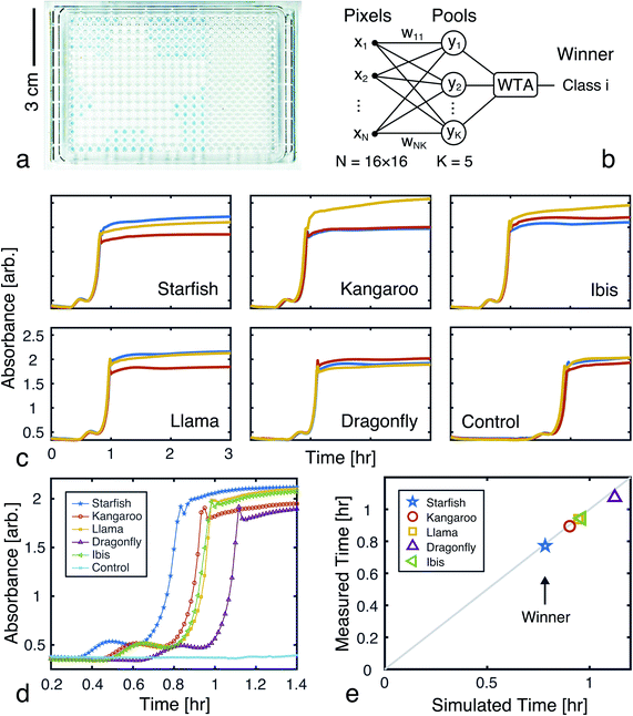
A 256-pixel binary image of a starfish, shown in Fig. 7c, was written to a 384-well plate using catalyst presence/absence encoding. The data plate preparation began by first dispensing Vs = 9.5 μL of solvent (6% methanol in water) to all wells. Wells corresponding to white pixels (xn = 1) received an additional Vd = 200 nL of 2×-diluted pre-reacted solution, nominally containing Do = 618 mM of catalyst. Wells corresponding to black pixels (xn = 0) had no catalyst added. An image of the resulting data plate is shown in Fig. 8a, where a faint blue color can be seen in the wells that contain catalyst (c = 12.742 mM).
The weights for each considered class were applied to the starfish image, resulting in 5 separate pools. A small volume (Vp = 1 μL) from each output pool was transferred, in triplicate, to wells on a new 384-well plate. To begin the CuAAC reactions, Vr = 50 μL of starting reagent solution was added to each well. The plate was promptly loaded into a UV-vis reader to track the progression of the reactions.
Absorbance measurements were taken every 60 seconds over the course of 8 hours. The measured signals are shown in Fig. 8c and compared in Fig. 8d. Consistent with the simulation, the ‘starfish’ pool was the first reaction to complete. The runner up, kangaroo, was 6.5 minutes behind. On average, measured transition times deviated from simulations by 2% (Fig. 8e).
Perspectives for chemical computing
DNA has often been the chemistry of choice for many developments in chemical computing,10,21,22,45–50 and it will continue to provide a powerful foundation for molecular-scale computation. DNA reaction networks benefit from the sequence-specificity of hybridization reactions and the availability of numerous catalytic enzymes. Strand displacement reactions, for instance, have been used to perform winner-take-all classification of 10 × 10 pixel binary images.22 However, because the operations rely on specific DNA sequences, a relatively large number of reagents must be designed and synthesized a priori. In contrast, the CuAAC reaction requires only three inputs, allowing for rapid re-configuration. Furthermore, DNA is often constrained to biologically relevant conditions (e.g. pH, temperature, salinity). Opportunities to utilize a broader range of catalytic reactions, which use fewer reagents or operate outside of physiological conditions, may open up new avenues for chemical computing.Autocatalytic processes, with their nonlinear response and input–output self-similarity, represent an attractive substrate for chemical based computing. In this work, we have shown, with a simple single-layer WTA network, how the kinetics of an autocatalytic reaction could be exploited for in chemico image classification. In the future, autocatalytic computation could be extended to more complicated architectures, such as a multi-layered WTA network that uses multiple rounds of volumetric pooling. Because the CuAAC reaction progress can be monitored through visible color changes there is no need for additional reporter molecules. Additionally, since the CuAAC reaction involves a reactive copper species (Cu(I)), it could be coupled to other reactions which would influence triazole production, potentially allowing for more complex and dynamic operations.
Conclusions
In summary, we designed and implemented a simple neural network using an array of autocatalytic reactions. This research extends previous chemical computing efforts which utilized non-reactive mixtures and were limited to linear mathematical operations.26 Here, we adapted the autocatalytic CuAAC reaction to serve as the nonlinear activation function needed for WTA classification. This work represents unique experimental progress towards a fully liquid-phase chemical classifier, in a non-biological chemistry. We anticipate that autocatalytic reaction networks will play a critical role in the future development of advanced chemical-domain computing systems.Methods
Materials and reagents
All solutions were prepared using in-house deionized water (Millipore Milli-Q), having a resistivity of 18.2 MΩ cm at 25 °C, and HPLC-grade methanol (>99%, Fisher Scientific, Waltham, MA). The CuAAC reaction was done, in a solvent comprised of 6% methanol and 94% water, using 2-azidoethanol (98%, Santa Cruz Biotechnology Inc, Dallas, TX) as the azide, tripropargylamine (98%, Sigma Aldrich, Natick, MA) as the alkyne, and copper(II) sulfate (>99%, Sigma Aldrich, Natick, MA) as the source of copper ions. The reactions were conducted at room temperature, in sealed well plates and cuvettes to prevent evaporation. Low dead volume 384-well microplates made of cyclic olefin copolymer (LP-0200, Labcyte Echo) and 384-well microplates made of polypropylene were used for high throughput experiments (PP-0200, Labcyte Echo).Instrumentation and analysis
An Echo 550 (Labcyte) acoustic fluid handler was used to perform the volume transfers for the high throughput experiments. Custom Python scripts were used to generate fluid handling instructions. Individual UV-vis measurements were taken with the Cary 50 (Varian), while the Synergy HTX (BioTek) platereader was used for arrayed measurements. Custom MATLAB scripts were used for network design, data analysis, and visualization.Network training
The objective of training is to produce a matrix of weights which maximize the accuracy of the WTA network. In order to correctly identify an image, the pool for its associated class should transition before that of any other class. Because volumetric multiply-accumulate operations correspond to positive weights26 and since there is an imposed upper limit (Vu) on the transfer volume, weight values can be specified relative to the transfer limit, such that they fall between 0 and 1.To accommodate these constraints, the network is trained similarly to a self-organizing map,51 where weights are iteratively tuned to be more similar to input data. A benefit of training the weights on the inputs, rather than on the outputs of the activation function, is that the weights are independent of specific chemical conditions and only require the time to transition to be monotonic in initial catalyst concentration.
If a weight vector (![[w with combining right harpoon above (vector)]](https://www.rsc.org/images/entities/i_char_0077_20d1.gif) i) is trained to identify class i, it should look more like the data (
i) is trained to identify class i, it should look more like the data (![[x with combining right harpoon above (vector)]](https://www.rsc.org/images/entities/i_char_0078_20d1.gif) ) from class i than a weight vector from any other class:
) from class i than a weight vector from any other class:
‖![[w with combining right harpoon above (vector)]](https://www.rsc.org/images/entities/i_char_0077_20d1.gif) i − i − ![[x with combining right harpoon above (vector)]](https://www.rsc.org/images/entities/i_char_0078_20d1.gif) ‖2 < ‖ ‖2 < ‖![[w with combining right harpoon above (vector)]](https://www.rsc.org/images/entities/i_char_0077_20d1.gif) j − j − ![[x with combining right harpoon above (vector)]](https://www.rsc.org/images/entities/i_char_0078_20d1.gif) ‖2, ∀j ≠ i ‖2, ∀j ≠ i | (13) |
 This inequality can be summed across the remaining K − 1 classes to yield:
 | (14) |
 | (15) |
![[x with combining right harpoon above (vector)]](https://www.rsc.org/images/entities/i_char_0078_20d1.gif) is data from class i. Averaging the losses over the training data, we arrive at the following objective:
is data from class i. Averaging the losses over the training data, we arrive at the following objective: | (16) |
![[x with combining right harpoon above (vector)]](https://www.rsc.org/images/entities/i_char_0078_20d1.gif) m).
m).
We want to find the weight matrix (W) that minimizes this objective (F). Taking the partial derivative of the objective, for feature n and class k, yields:
 | (17) |
 | (18) |
A MATLAB implementation of the training routine is provided in the ESI (Listing S1†) and is also available on Github: github.com/Chris3Arcadia/AutocatalyticWTA. In addition to the experimentally tested network, one hundred 5-class WTA networks (see Fig. S10 and Table S1†) and one 9-class WTA network (see Fig. S11 and S12†) were trained and evaluated in silico to test the proposed classification scheme.
Author contributions
C. E. A., A. D., K. O., and S.-L. C. performed experiments. C. E. A. and K. O. analyzed data. C. E. A and H. K. performed simulations. C. R., E. K., S. R., B. M. R., and J. K. R. provided direction and oversight. C. E. A., A. D., K. O., and J. K. R. drafted the paper. All authors provided notes and edits to the paper.Conflicts of interest
The authors declare that they have no conflicts of interest.Acknowledgements
This research was supported by funding from the Defense Advanced Research Projects Agency (DARPA W911NF-18-2-0031). The views, opinions and/or findings expressed are those of the authors and should not be interpreted as representing the official views or policies of the Department of Defense or the U.S. Government. This work was also supported in part by the National Science Foundation under Grant No. 1941344.Notes and references
- R. Plasson, A. Brandenburg, L. Jullien and H. Bersini, J. Phys. Chem. A, 2011, 115, 8073–8085 CrossRef CAS PubMed.
- P. Richard, FEMS Microbiol. Rev., 2003, 27, 547–557 CrossRef CAS PubMed.
- C. Thron, Biophys. Chem., 1996, 57, 239–251 CrossRef CAS PubMed.
- N. A. Thornberry and Y. Lazebnik, Science, 1998, 281, 1312–1316 CrossRef CAS PubMed.
- P. v. Nies, I. Westerlaken, D. Blanken, M. Salas, M. Mencía and C. Danelon, Nat. Commun., 2018, 9, 1583 CrossRef PubMed.
- D. H. Lee, K. Severin and M. R. Ghadiri, Curr. Opin. Chem. Biol., 1997, 1, 491–496 CrossRef CAS PubMed.
- W. Hordijk, J. Hein and M. Steel, Entropy, 2010, 12, 1733–1742 CrossRef CAS.
- A. M. Zador, Nat. Neurosci., 2000, 3, 1167 CrossRef CAS PubMed.
- F. Simini, 2016, arXiv:1602.09070.
- L. Adleman, Science, 1994, 266, 1021–1024 CrossRef CAS PubMed.
- F. L. Carter, Phys. D, 1984, 10, 175–194 CrossRef.
- G. M. Church, Y. Gao and S. Kosuri, Science, 2012, 337, 1628 CrossRef CAS PubMed.
- L. Organick, S. D. Ang, Y.-J. Chen, R. Lopez, S. Yekhanin, K. Makarychev, M. Z. Racz, G. Kamath, P. Gopalan, B. Nguyen, C. N. Takahashi, S. Newman, H.-Y. Parker, C. Rashtchian, K. Stewart, G. Gupta, R. Carlson, J. Mulligan, D. Carmean, G. Seelig, L. Ceze and K. Strauss, Nat. Biotechnol., 2018, 36, 242–248 CrossRef CAS PubMed.
- L. Anavy, I. Vaknin, O. Atar, R. Amit and Z. Yakhini, Nat. Biotechnol., 2019, 37, 1229–1236 CrossRef CAS PubMed.
- N. F. König, A. A. Ouahabi, L. Oswald, R. Szweda, L. Charles and J.-F. Lutz, Nat. Commun., 2019, 10, 3774 CrossRef PubMed.
- C. E. Arcadia, E. Kennedy, J. Geiser, A. Dombroski, K. Oakley, S.-L. Chen, L. Sprague, M. Ozmen, J. Sello, P. M. Weber, S. Reda, C. Rose, E. Kim, B. M. Rubenstein and J. K. Rosenstein, Nat. Commun., 2020, 11, 691 CrossRef CAS PubMed.
- J. K. Rosenstein, A. Dombroski, K. Oakley, S. L. Chen, H. Tann, B. M. Rubenstein, C. Rose, S. Reda, P. M. Weber, E. Kim, J. Sello, J. Geiser, E. Kennedy and C. Arcadia, IEEE Trans. Nanobiosci., 2020, 1 Search PubMed.
- J. Hasty, D. McMillen and J. J. Collins, Nature, 2002, 420, 224–230 CrossRef CAS PubMed.
- H. Kim, D. Bojar and M. Fussenegger, Proc. Natl. Acad. Sci. U. S. A., 2019, 116, 201821740 Search PubMed.
- L. Qian, E. Winfree and J. Bruck, Nature, 2011, 475, 368–372 CrossRef CAS PubMed.
- X. Song, A. Eshra, C. Dwyer and J. Reif, RSC Adv., 2017, 7, 28130–28144 RSC.
- K. M. Cherry and L. Qian, Nature, 2018, 559, 370–376 CrossRef CAS PubMed.
- N. G. Rambidi, Biosystems, 1995, 35, 195–198 CrossRef CAS PubMed.
- J. Gorecki, K. Gizynski, J. Guzowski, J. N. Gorecka, P. Garstecki, G. Gruenert and P. Dittrich, Philos. Trans. R. Soc., A, 2015, 373, 20140219 CrossRef PubMed.
- A. Pandi, M. Koch, P. L. Voyvodic, P. Soudier, J. Bonnet, M. Kushwaha and J.-L. Faulon, Nat. Commun., 2019, 10, 3880 CrossRef PubMed.
- C. E. Arcadia, H. Tann, A. Dombroski, K. Ferguson, S. L. Chen, E. Kim, C. Rose, B. M. Rubenstein, S. Reda and J. K. Rosenstein, IEEE International Conference on Rebooting Computing, 2018, 1–9 Search PubMed.
- R. Brijder, Nat. Comput., 2019, 18, 119–137 CrossRef CAS.
- D. Blount, P. Banda, C. Teuscher and D. Stefanovic, Artif. Life, 2017, 23, 295–317 CrossRef PubMed.
- C. Rose, S. Reda, B. Rubenstein and J. Rosenstein, 2018 IEEE International Symposium on Information Theory (ISIT), 2018, pp. 2236–2240 Search PubMed.
- P. Banda, C. Teuscher and M. R. Lakin, Artif. Life, 2013, 19, 195–219 CrossRef PubMed.
- P. Banda and C. Teuscher, Artificial Life Conference Proceedings, 2014, vol. 14, pp. 482–489 Search PubMed.
- Y. LeCun, L. Bottou, Y. Bengio and P. Haffner, Proc. IEEE, 1998, 86, 2278–2324 CrossRef.
- J. I. Steinfeld, J. S. Francisco and W. L. Hase, Chemical kinetics and dynamics, Prentice Hall Englewood Cliffs, New Jersey, 1989, vol. 3 Search PubMed.
- B. Kia, J. F. Lindner and W. L. Ditto, Philos. Trans. R. Soc., A, 2017, 375, 20160222 CrossRef PubMed.
- G. Hinton, L. Deng, D. Yu, G. E. Dahl, A. Mohamed, N. Jaitly, A. Senior, V. Vanhoucke, P. Nguyen, T. N. Sainath and B. Kingsbury, IEEE Signal Process. Mag., 2012, 29, 82–97 Search PubMed.
- V. Nair and G. E. Hinton, ICML, 2010, 807–814 Search PubMed.
- R. A. Evans, Aust. J. Chem., 2007, 60, 384–395 CrossRef CAS.
- H. C. Kolb, M. G. Finn and K. B. Sharpless, Angew. Chem., Int. Ed., 2001, 40, 2004–2021 CrossRef CAS PubMed.
- S. N. Semenov, L. Belding, B. J. Cafferty, M. P. Mousavi, A. M. Finogenova, R. S. Cruz, E. V. Skorb and G. M. Whitesides, J. Am. Chem. Soc., 2018, 140, 10221–10232 CrossRef CAS PubMed.
- T. R. Chan, R. Hilgraf, K. B. Sharpless and V. V. Fokin, Org. Lett., 2004, 6, 2853–2855 CrossRef CAS PubMed.
- D. Döhler, P. Michael and W. H. Binder, Macromolecules, 2012, 45, 3335–3345 CrossRef.
- S. Kaski and T. Kohonen, Neural Network., 1994, 7, 973–984 CrossRef.
- W. Maass, Neural Comput., 2006, 12, 2519–2535 CrossRef PubMed.
- B. Marlin, K. Swersky, B. Chen and N. Freitas, Proceedings of the Thirteenth International Conference on Artificial Intelligence and Statistics, Chia Laguna Resort, Sardinia, Italy, 2010, pp. 509–516 Search PubMed.
- R. Lipton, Science, 1995, 268, 542–545 CrossRef CAS PubMed.
- B. Yurke, A. J. Turberfield, A. P. Mills, F. C. Simmel and J. L. Neumann, Nature, 2000, 406, 605–608 CrossRef CAS PubMed.
- D. Woods, D. Doty, C. Myhrvold, J. Hui, F. Zhou, P. Yin and E. Winfree, Nature, 2019, 567, 366–372 CrossRef CAS PubMed.
- N. Mamet, G. Harari, A. Zamir and I. Bachelet, Comput. Biol. Chem., 2019, 107122 CrossRef CAS PubMed.
- R.-R. Gao, T.-M. Yao, X.-Y. Lv, Y.-Y. Zhu, Y.-W. Zhang and S. Shi, Chem. Sci., 2017, 8, 4211–4222 RSC.
- X. Lin, S. Yang, D. Huang, C. Guo, D. Chen, Q. Yang and F. Li, Chem. Sci., 2020, 11, 9617–9622 RSC.
- T. Kohonen, Proc. IEEE, 1990, 78, 1464–1480 CrossRef.
- S. Ruder, 2016, arXiv:1609.04747.
Footnote |
| † Electronic supplementary information (ESI) available: Details about the source code, image database, class selection, classifier training, and additional network simulations are provided (PDF). See DOI: 10.1039/d0sc05860b |
| This journal is © The Royal Society of Chemistry 2021 |

