Transmol: repurposing a language model for molecular generation

Abstract

Recent advances in convolutional neural networks have inspired the application of deep learning to other disciplines. Even though image processing and natural language processing have turned out to be the most successful, there are many other domains that have also benefited; among them, life sciences in general and chemistry and drug design in particular. In concordance with this observation, from 2018 the scientific community has seen a surge of methodologies related to the generation of diverse molecular libraries using machine learning. However to date, attention mechanisms have not been employed for the problem of de novo molecular generation. Here we employ a variant of transformers, an architecture recently developed for natural language processing, for this purpose. Our results indicate that the adapted Transmol model is indeed applicable for the task of generating molecular libraries and leads to statistically significant increases in some of the core metrics of the MOSES benchmark. The presented model can be tuned to either input-guided or diversity-driven generation modes by applying a standard one-seed and a novel two-seed approach, respectively. Accordingly, the one-seed approach is best suited for the targeted generation of focused libraries composed of close analogues of the seed structure, while the two-seeds approach allows us to dive deeper into under-explored regions of the chemical space by attempting to generate the molecules that resemble both seeds. To gain more insights about the scope of the one-seed approach, we devised a new validation workflow that involves the recreation of known ligands for an important biological target vitamin D receptor. To further benefit the chemical community, the Transmol algorithm has been incorporated into our cheML.io web database of ML-generated molecules as a second generation on-demand methodology.

---

1 Introduction

Chemistry is frequently referred to as a “central science” for its key role in advancing technological progress and human well-being through the design and synthesis of novel molecules and materials for energy, environmental, and biomedical applications.

Medicinal chemistry is a highly interdisciplinary field of science that deals with the design, chemical synthesis, and mechanism of action of biologically active molecules as well as their development into marketed pharmaceutical agents (i.e. drugs). The creation of new drugs is an incredibly hard and arduous process, one of the key reasons being the fact that the ‘chemical space’ of all possible molecules is extremely large and intractable. On account of estimates that the chemical space of molecules with pharmacological properties is in the range of 10²³ to 10⁶⁰ compounds,¹ this order of magnitude leaves the work of finding new drugs outside the reach of manual labor.

To cure a particular disease, medicinal chemists need to determine molecules that are active and selective towards specific biological targets while keeping the risks of negative side effects minimal.^2–5 As the number of molecules that require testing to identify an ideal drug candidate constantly increases, it raises the overall cost of the drug discovery process.⁶ Therefore, the need for algorithms that are able to narrow down and streamline these efforts has recently emerged. Specifically, computer algorithms can assist with creating new virtual molecules,^7,8 performing molecule conformation analysis^9,10 as well as molecular docking^11,12 to determine the affinity of novel and known molecules towards specific biological targets.

With respect to molecular generation, the conventional non-neural algorithms heavily rely on external expert knowledge to design candidate molecules. In this context, expert knowledge may consist of molecular fragments that can be “mixed and matched” to produce a set of novel molecules.^13–18 However, the resulting molecules might be difficult to synthesize. Consequently, another type of expert knowledge i.e. known chemical reactions can then be added.^19,20 In this way the “mix and match” approach will be constrained with a specific set of rules to maximize the chances that any molecule that is produced can be synthesized.²¹ The obvious drawback of relying on external knowledge is that it may restrict access to unknown and/or not yet populated regions of chemical space.

An alternative approach to this problem are neural algorithms that are inherently data-driven. This means that such algorithms do not rely on expert knowledge and hence derive insights from the data itself. Such approaches can be applied in supervised and unsupervised settings.^22–24 Supervised algorithms use artificial neural networks for the prediction of molecular properties^25,26 or reaction outputs.²⁷ Most unsupervised algorithms are aimed at molecular generation and drug design.^8,22,28–48

When automating molecular search, a natural question that arises is how molecules, a physical collection of atoms that are arranged in 3D space, can be represented. In the late 1980s, the simplified molecular input line-entry system (SMILES) emerged, which aims to create a molecular encoding that is computationally efficient to use and human readable.⁴⁹ The original encoding is based on 2D molecular graphs. Intended application areas are fast and compact information retrieval and storage. With the rise of machine learning algorithms in chemistry, the SMILES representation has been widely adopted by researchers for chemical space modeling tasks.

The task of generating more SMILES strings having an input string can be viewed as a language modelling task. The model takes an arbitrary length SMILES string (seed molecule) and returns arbitrary long SMILES strings – the general class of such models is called Seq2Seq. First used by Google,⁵⁰ it is currently one of the most popular approaches for machine translation. The Seq2Seq architecture can be summarized as follows: an encoder produces a context vector that is later passed to the decoder for the generation in auto-regressive fashion.⁵⁰

As the building blocks of the encoder and decoder could be neural networks with various architectures, researchers have experimented with a number of techniques: generative adversarial networks,^{30,38,44,45,51} variational autoencoders,^39,52 and recurrent neural networks.^53,54 However, the use of attention mechanisms has, to the best of our knowledge, so far been left unexplored. Here we aim to fill this gap and investigate the applicability of attention to molecular generation.

One of the distinctive features of attention is that, unlike for example RNN-type models which have a fixed amount of memory, attention mechanisms allow varying the length of the latent vector so that the input information does not have to be compressed into a fixed-length vector. In other words, attention will provide a varying length vector that contains the related information regarding all input nodes (i.e. SMILES characters, atoms, rings and branching info, etc.). Thus, in case of the standard one-seed approach the outcome strives to replicate the input, which means that upon injecting some variability into the model the algorithm can be tuned to attain a focused library of close-seed analogues. In order to switch from this genuinely input-guided mode to a more diversity-driven mode, we have come up with the idea of a two-seed approach. This novel approach is not only capable of generating diversified molecular libraries by assembling structures that resemble both seeds, but it also provides a Euclidean navigation framework of the latent space and can thus lead to further insights during the exploration of chemical space. The resulting Transmol algorithm comprising the two above described generation modes has been incorporated into the cheml.io⁵⁵ website with the aim to make these findings accessible to a wider audience.

2 Dataset

In this paper, we have used the MOSES benchmark⁵⁶ along with the molecular datasets it provides. Overall, the MOSES benchmark contains three datasets: training set, test set, and scaffold test set, which consist of 1.6M, 176k, and 176k samples, respectively.

The first dataset was used to train the model. During this stage the model learns to interpolate between each molecule and constructs a latent space. This latent space acts as a proxy distribution for molecules, and can be employed to sample new molecules.

The testing dataset consists of molecules that are not present in the training data. It is used to evaluate the output of the generative model.

The scaffold testing set consists of scaffolds that are not present in the training and testing datasets. This dataset is used to check if the model is able to generate new scaffolds, i.e. unique molecular features, or whether the model simply reuses parts of the previously seen molecules to generate new ones.

2.1 Data augmentation

In order to increase the variability of our data, we have used data augmentation by means of SMILES enumeration. This simple, yet effective technique has recently been introduced by Arús-Pous et al.:⁵⁷ While a molecule can be mapped to its unique canonical SMILES string, a whole set of non-unique SMILES strings can also be produced depending on the starting point where the algorithm will begin the translation. Such data augmentation have been reported to improve the generalization of the latent space and to increase the diversity of the output molecules.

3 Methods

While the Seq2Seq architecture is successful in a whole range of applications, the disadvantage of this architecture is that it uses fixed length vectors: it is bound (bottlenecked) by the size of the vector and sub-optimal for long sequences.

For this work, we have employed a vanilla transformer model introduced by Vaswani et al.⁵⁸ (see Fig. 1 for a pictorial representation of the architecture). All code for this study has been written in Python and is publicly available on GitLab.⁵⁹ The initial transformer code was adapted from the annotated version.⁶⁰ A vanilla transformer consists of two parts: an encoder and a decoder. The encoder (see left dashed block of Fig. 1) maps input to the latent representation z. The decoder (see dashed block on the right of Fig. 1), accepts z as an input and produces one symbol at a time. The model is auto-regressive, i.e. to produce a new symbol it requires previous output as an additional input.

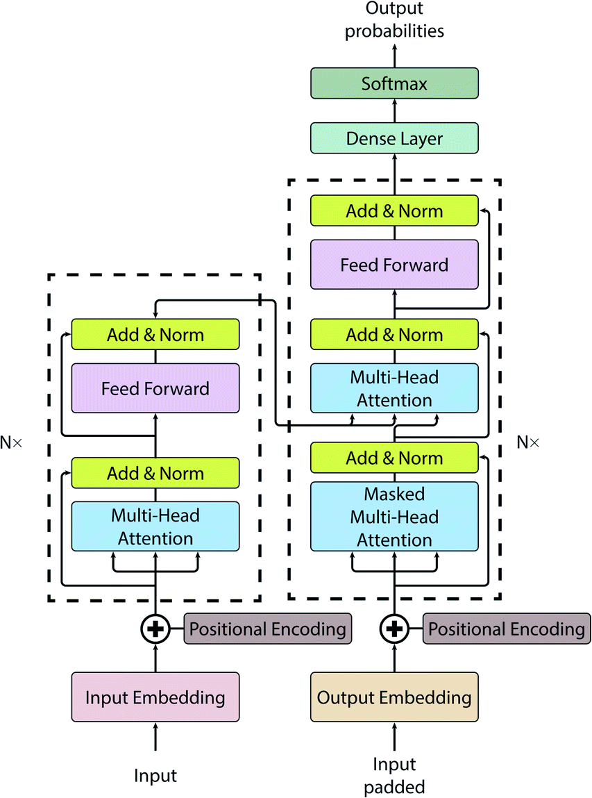Fig. 1 A vanilla transformer architecture.

The notable attribute of this architecture is the use of attention mechanisms throughout the whole model. While earlier models have been using attention only as an auxiliary layer, having some kind of recurrent neural networks (RNN) like a gated recurrent unit (GRU) or long short-term memory (LSTM), or a convolutional neural network (CNN), the transformer consists primarily of attention layers.

The attention mechanism can be seen as a function of query Q, key K and value V, where the output is a matrix product of Q, K, V using the following function:

is used to identify the relevant parts of the input with respect to the input, namely self-attention. The scaled dot-product attention consists of 3 main matrices Q, K and V. The transformer computes these 3 matrices in the embedding layers. All 3 matrices are not fixed and are learnable. After embedding the layers will receive the output of the previous layers. The dot product is computed between Q and all keys to compute a “relevance” score. A higher “relevance” score means that after normalizing and applying the softmax, the lowest scores will become zeros. The important feature of the self-attention used in this model is that it does not use fixed length vectors. While Seq2Seq models with RNN⁵⁴ attempt to compress all information into a fixed-length context, self-attention mechanisms employed in this model have access to the whole context and able to selectively focus only on the most important parts. Vice versa, it allows to disregard less important parts of the query and to filter the noise. Most importantly, attention mechanisms are differentiable and hence can be learned from data as can be seen from eqn (1) for a description of the scaled dot-product attention layer. The multi-head attention layer consists of h instances of scaled dot-product attention layers that are then concatenated and passed to the dense layer.

The parameter setup of the original paper has been employed here, i.e. the number of stacked encoder and decoder layers is N = 6, all sublayers produce an output of d_model = 512, with the dimensionality of the inner feed-forward layer being d_ff, number of attention heads h = 6, and dropout d = 0.1. The learning rate is specified by the optimization function of the original manuscript with the following modified hyperparameters: warmup steps are set to 2000, factor is 1, the batch size is 1200 and the training was performed for 16 epochs. The rest of the hyperparameters were adopted unchanged from the original paper, i.e. we have not optimized the other hyperparameters leaving them as in the original paper. One of the reasons are the large number of hyperparameters and limited computing resources. Please note that further hyperparameter optimization may thus improve the performance of the model.

3.1 Sampling from the latent space

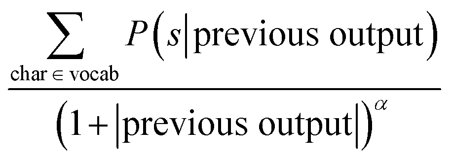
To sample a novel molecule from the model, a seed SMILES string is needed in order to provide a context for the decoder. Then the decoding process is started by supplying a special starting symbol. After that the decoder provides an output and a first symbol is generated. In order to obtain the next symbol the previous characters are provided to the decoder. The decoding process stops when the decoder either outputs a special terminal symbol or exceeds the maximum length. There are several techniques available that specify how the output of the decoder is converted to the SMILES character such as a simple greedy search or a beam search, among others.

3.1.1 Greedy search. Since the decoder provides output probabilities, a naïve approach would be to use a greedy algorithm by always picking the symbol with the highest probability. However, this is not optimal as picking the most probable symbol at each step leads for a relatively small library. In addition, the greedy search does not guarantee that the final resulting string has the highest conditional probability. Moreover, unless stochastic sampling is used (here a probability vector is used as the basis for the distribution and then sampled), the result of the greedy search is deterministic and corresponds to the “reconstruction accuracy” based on our training procedure.

3.1.2 Beam search. To improve upon the greedy search, a beam search has been employed as an alternative. The beam search can be seen as an improved greedy search. While the greedy search picks only one symbol at a time, the beam search picks the N most probable ones. Fig. 2 illustrates the beam search with a beam width N = 3; the stroke width indicates the probability. To guide the selection process of the beam search we have used the following reward function:
where char is a possible symbol for the beam search to pick, vocab is the set of all possible characters, previous output is an ordered list of symbols picked by the beam search prior to picking the current one and α is a parameter of the beam search that regulates the length of the string. Low α discourages long strings while high α encourages long strings.

Fig. 2 Overview of the beam search with a beam width of N = 3.

3.2 Injecting variability into model

To explore the molecules that are located near the seed molecule in the latent space, we have used two techniques that allow us to sample from the seed cluster: addition of Gaussian noise to z and the use of temperature.

3.2.1 Gaussian noise. To increase the variability of the model we are adding Gaussian noise with a mean of μ and standard deviation σ to the latent vector z before it is fed to the decoder. In our study, parameters for μ and σ were 1 and 1.06 respectively.

3.2.2 Temperature. Another technique to improve variability is to apply temperature to the output vector right before applying the softmax function. Temperature T is a value from 0 to ∞. As T → ∞ all characters have the same probability of being the next symbol. For T → 0 the most probable symbol has a higher probability of being selected. The resulting smoothed distribution increases the variability of the sampling. In our study the parameter for temperature was fixed as 0.5.

3.3 MOSES benchmark

MOSES is an established benchmarking system for the evaluation of molecular generation algorithms.⁵⁶ It contains several implemented molecular generation frameworks as well as a range of metrics to compare molecular outputs. The baseline models can be roughly divided into two categories: neural and non-neural. Neural methods use artificial neural networks to learn the distribution of the training set. A whole range of them are implemented, namely character-level recurrent neural network (CharRNN),^35,61 variation autoencoder (VAE),^32,62,63 adversarial autoencoder (AAE),^62,64 junction tree VAE (JT-VAE),³⁶ and latent vector based generative adversarial network (LatentGAN).⁶⁵ Non-neural baselines include the n-gram generative model (NGram), the hidden Markov model (HMM), and a combinatorial generator. Non-neural baselines are conceptually simpler than neural ones. The NGram model collects the frequency of the n-grams in the training dataset and uses the resulting distribution to sample new strings. For instance, during counting of a 2 gram, the model will inspect individual SMILES strings and record their statistics. For the string “C1CCC1C” the following statistics will be gathered C1:2, CC:2, 1C:2. Later this type of information will be normalized and used for sampling. HMM uses the Baum–Welch algorithm for distribution learning. The combinatorial generator uses BRICS fragments of the training dataset. These fragments are the substructures of molecules that are cut according to a set of rules for the breaking of retrosynthetically interesting chemical substructures (BRICS).⁶⁶ In order to sample, combinatorial generator randomly connects several such fragments.

Several metrics are provided by the MOSES benchmark. Uniqueness shows the proportion of generated molecules that are within the training dataset. Validity describes the proportion of generated molecules that are chemically sound, as checked by RDKit.⁶⁷ Internal diversity measures whether the model samples from the same region of chemical space, i.e. producing molecules that are valid and unique but only differ in a single atom. Filters measures the proportion of a generated set that passes a number of medical filters. Since the training set contains only molecules that pass through these filters, it is an implicit constraint imposed on the algorithm.

Fragment similarity (Frag) measures the similarity of the BRICS fragments distribution contained in the reference and generated sets. If the value is 1, then all fragments from the reference set are present in the generated one. If the value is 0, then there are no overlapping fragments between the generated and reference sets. Scaffold similarity (Scaff) is similar to Frag, but instead of BRICS fragments, Bemis–Murcko scaffolds are used for comparison. The range of this metric is analogous to Frag. Similarity to the nearest neighbor (SNN) is a mean Tanimoto distance between a molecule in the reference set and its closest neighbor from the generated set. One of the possible interpretations of this metric is precision; if the value is low, it means that the algorithm generates molecules that are distant from the molecules in the reference set. The range of this metric is [0, 1]. Fréchet ChemNet Distance (FCD) is a metric that correlates with internal diversity and uniqueness. It is computed using the penultimate layer of the ChemNet, a deep neural network that is trained for the prediction of biological activities. All four aforementioned metrics have also been compared to the scaffold test dataset.

3.4 A workflow for Transmol validation via the recreation of known vitamin D receptor ligands

In order to demonstrate the viability of our model we have designed a small retrospective study that is aiming at the recreation of known ligands of the Vitamin D Receptor (VDR).

VDR is a member of the nuclear receptor superfamily, a zinc-finger transcriptional factor and a canonical receptor for its most active secosteroid 1α,25-dihydroxyvitamin D₃ (1,25D₃) (Fig. 3A). It has also been established as sensor for steroid acids such as lithocholic acid (Fig. 3B) predominantly acting as an activator of the detoxification pathway for them in the human colon through regulation of cytochrome P450 monooxygenases e.g. CYP3A4. The classical VDR physiology involves the activation and regulation of divers processes such as mineral homeostasis, cellular proliferation and differentiation and the modulation of native and adaptive immunity.⁶⁸ Hence, their dysfunction may be connected to serious maladies making VDR suitable for effective drug-target development.⁶⁹ To date more than 3000 vitamin D (VD) analogues have been synthesized largely due to the side effects of 1,25D₃ such as hypercalcemia with some of them belonging to a completely new group of analogues called non-steroidal VD analogues of which an example is shown in Fig. 3C.⁷⁰

Fig. 3 Structural representations of the main VDR ligands groups. (A) the secosteroid 1,25D₃ bound to ratVDR (PDBID: 1RK3), (B) steroid acid e.g. lithocholic acid (LCA) bound to ratVDR (PDBID: 3W5P) and (C) non-steroidal analogue YR301 bound to ratVDR (PDBID: 2ZFX). All crystal structure were superimposed to 1RK3, the critical amino acid contacts are highlighted in all structures.

The dataset for recreating VDR ligands was extracted from the ZINC database.⁷¹ The ZINC database is a reliable curated database with all compounds available for purchase and testing. From this database 418 VDR ligands have been selected. After canonicalizing and stripping the stereoisomeric information from these molecules, 210 SMILES strings remained. We further divided these 210 molecules into approximately equal size training and test sets. The training data was used for model fine-tuning and subsequently as seed molecules to create focused libraries of potential VDR ligands. The test set was used as a reference for the comparison of Transmol-generated molecules. While the sample size of this dataset is comparatively small, it is composed of only several subsets of VDR ligands with each subset containing molecules that are structurally similar to each other. Therefore, we theorize that Transmol may be able to extract enough information from the training data to recreate previously known VDR ligands and thus mimic the process of creating new ones. To reduce the impact of randomness we perform this procedure ten times.

A detailed workflow for examining the recreation of known VDR ligands with Transmol can be summarized in the following way:

(1) Acquire 418 known VDR ligands from the ZINC database.

(2) Bring them into canonical form by discarding the stereoisomeric information reduced the set to 210 molecules.

(3) Randomly sample 100 structures and use them as a training set. Remaining 110 constitute the test set.

(4) Use the training set to fine tune Transmol. Fine tuning is a common technique in deep learning. The idea is that instead of training a new model from scratch we can use a set of model parameters trained on a large dataset, and then perform additional training on a smaller dataset.

(5) Use a subset of training molecules as seeds for Transmol (30 randomly selected ligands from the training set).

(6) Compare Transmol output to test set molecules and record overlap.

(7) Repeat steps 3 to 6 ten times.

4 Results and discussion

In this section, we describe major results and insights that were obtained during the implementation of our model and while disseminating its output. It starts with analyzing the outcome of a standard one-seed approach with the MOSES benchmark and medicinal chemistry filters followed by the application of single seed settings for the regeneration of known VDR ligands. It also outlines a novel two-seed approach that targets the generation of diversified molecular libraries. In this regard the two-seed approach is complementary to the standard one-seed approach which works best for the acquisition of focused libraries of close seed's analogues.

4.1 Creating a focused library with one seed molecule

The standard Transmol settings involve the generation of a focused library using a single seed molecule. Fig. 4 provides the graphical overview of this process indicating that upon optimizing the sampling hyperparameters (see ESI† for details) the single-seed approach yields the molecular library of close structural analogues of the seed. Overall, we have fed Transmol with 8000 seed molecules gathered from the MOSES test set resulting in the generation of 8000 focused libraries. The combined outcome has then been bench-marked with MOSES⁵⁶ and analyzed using various medicinal chemistry filters in order to compare Transmol with other generative algorithms.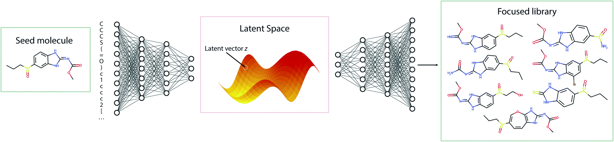

Fig. 4 The general pipeline of the sampling process for the one-seed approach.

4.1.1 Bench-marking Transmol with MOSES. According to Table 1, Transmol has demonstrates the greatest internal diversity (IntDiv₁ and IntDiv₁) across all other baseline methods within MOSES. It can be also observed that among the neural algorithms Transmol demonstrates the greatest proportion of novel molecules, that are not present in the training dataset. Another important observation is that Transmol's internal diversity score exceeds that of the training dataset. This observation might indicate the ability of Transmol to generalize well on the previously unseen data.

Table 1 Performance metrics for baseline models: fraction of valid molecules, fraction of unique molecules from 1000 and 10 000 molecules, internal diversity, fraction of molecules passing filters (MCF, PAINS, ring sizes, charge, atom types), and novelty. Reported (mean ± std) over three independent model initializations. Arrows next to the metrics indicate preferable metric values (higher is better for all). CharRNN – character-level recurrent neural network, AAE – adversarial autoencoder, VAE – variational autoencoder, JTN-VAE – junction tree variational autoencoder, LatentGAN – latent vector based generative adversarial network, Transmol – transformer for molecules

Model	Valid (↑)	Unique@1k (↑)	Unique@10k (↑)	IntDiv (↑)	IntDiv2 (↑)	Filters (↑)	Novelty (↑)
Train	1	1	1	0.8567	0.8508	1	1
HMM	0.076 ± 0.0322	0.623 ± 0.1224	0.5671 ± 0.1424	0.8466 ± 0.0403	0.8104 ± 0.0507	0.9024 ± 0.0489	0.9994 ± 0.001
NGram	0.2376 ± 0.0025	0.974 ± 0.0108	0.9217 ± 0.0019	0.8738 ± 0.0002	0.8644 ± 0.0002	0.9582 ± 0.001	0.9694 ± 0.001
Combinatorial	1.0 ± 0.0	0.9983 ± 0.0015	0.9909 ± 0.0009	0.8732 ± 0.0002	0.8666 ± 0.0002	0.9557 ± 0.0018	0.9878 ± 0.0008
CharRNN	0.9748 ± 0.0264	1.0 ± 0.0	0.9994 ± 0.0003	0.8562 ± 0.0005	0.8503 ± 0.0005	0.9943 ± 0.0034	0.8419 ± 0.0509
AAE	0.9368 ± 0.0341	1.0 ± 0.0	0.9973 ± 0.002	0.8557 ± 0.0031	0.8499 ± 0.003	0.996 ± 0.0006	0.7931 ± 0.0285
VAE	0.9767 ± 0.0012	1.0 ± 0.0	0.9984 ± 0.0005	0.8558 ± 0.0004	0.8498 ± 0.0004	0.997 ± 0.0002	0.6949 ± 0.0069
JTN-VAE	1.0 ± 0.0	1.0 ± 0.0	0.9996 ± 0.0003	0.8551 ± 0.0034	0.8493 ± 0.0035	0.976 ± 0.0016	0.9143 ± 0.0058
LatentGAN	0.8966 ± 0.0029	1.0 ± 0.0	0.9968 ± 0.0002	0.8565 ± 0.0007	0.8505 ± 0.0006	0.9735 ± 0.0006	0.9498 ± 0.0006
Transmol	0.0694 ± 0.0004	0.9360 ± 0.0036	0.9043 ± 0.0036	0.8819 ± 0.0003	0.8708 ± 0.0002	0.8437 ± 0.0015	0.9815 ± 0.0004

---

As can be seen from Table 1, Transmol has a low validity score. One of the possible reasons is the architecture of the network. In architectures like autoencoders, or GANs the model is evaluated on how well it replicates the input during the training. However, in this case the model was learning the molecular space, by maximizing the likelihood of the next symbol. The aim of this work was to explore the molecular space through SMILES representations, and our model is successful in this task. It is natural that some areas of this space are uninhabited, i.e. contain only invalid SMILES. One of the possible solutions to amend the low validity would be the integration of autoencoders, or GAN parts into the model, since for these methods the accurate replication of the input is explicit. Another potential solution would be to optimize the model towards high validity.

Table 2 shows more sophisticated metrics that require the comparison of two molecular sets, reference and generated: Fréchet ChemNet Distance (FCD), similarity to the nearest neighbor (SNN), fragment similarity (Frag), and scaffold similarity (Scaff). In this table, we observe that Transmol has a relatively high FCD score compared to neural methods and a comparable or lower score in relation to non-neural algorithms. This is a surprising result that we have not anticipated considering the high scores of Transmol for internal diversity and relatively high scores for uniqueness. One of the probable reasons is that in our work we have used 8000 molecules as seeds out of ≈170000 molecules in the MOSES test set. As a result, we created 8000 focused libraries. The individual outputs exhibit high internal diversity, since each focused set results in unique molecules. In addition, these focused sets are diverse with respect to each other. The high FCD score indicates dissimilarity between our generated set and the MOSES test set. The reason for this is given by the fact that we are generating very focused libraries and therefore cannot (and do not need to) capture the whole variability of the MOSES test set. If the number of seed molecules would be increased substantially, the FCD value would decrease.

Table 2 Performance metrics for baseline models: Fréchet ChemNet Distance (FCD), similarity to a nearest neighbor (SNN), fragment similarity (Frag), and scaffold similarity (Scaff); reported (mean ± std) over three independent model initializations. Results for random test set (Test) and scaffold split test set (TestSF). Arrows next to the metrics indicate preferable metric values. CharRNN – character-level recurrent neural network, AAE – adversarial autoencoder, VAE – variational autoencoder, JTN-VAE – junction tree variational autoencoder, LatentGAN – latent vector based generative adversarial network, Transmol – transformer for molecules

Model	FCD (↓)		SNN (↑)		Frag (↑)		Scaf (↑)
	Test	TestSF	Test	TestSF	Test	TestSF	Test	TestSF
Train	0.008	0.4755	0.6419	0.5859	1	0.9986	0.9907	0
HMM	24.4661 ± 2.5251	25.4312 ± 2.5599	0.3876 ± 0.0107	0.3795 ± 0.0107	0.5754 ± 0.1224	0.5681 ± 0.1218	0.2065 ± 0.0481	0.049 ± 0.018
NGram	5.5069 ± 0.1027	6.2306 ± 0.0966	0.5209 ± 0.001	0.4997 ± 0.0005	0.9846 ± 0.0012	0.9815 ± 0.0012	0.5302 ± 0.0163	0.0977 ± 0.0142
Combinatorial	4.2375 ± 0.037	4.5113 ± 0.0274	0.4514 ± 0.0003	0.4388 ± 0.0002	0.9912 ± 0.0004	0.9904 ± 0.0003	0.4445 ± 0.0056	0.0865 ± 0.0027
CharRNN	0.0732 ± 0.0247	0.5204 ± 0.0379	0.6015 ± 0.0206	0.5649 ± 0.0142	0.9998 ± 0.0002	0.9983 ± 0.0003	0.9242 ± 0.0058	0.1101 ± 0.0081
AAE	0.5555 ± 0.2033	1.0572 ± 0.2375	0.6081 ± 0.0043	0.5677 ± 0.0045	0.991 ± 0.0051	0.9905 ± 0.0039	0.9022 ± 0.0375	0.0789 ± 0.009
VAE	0.099 ± 0.0125	0.567 ± 0.0338	0.6257 ± 0.0005	0.5783 ± 0.0008	0.9994 ± 0.0001	0.9984 ± 0.0003	0.9386 ± 0.0021	0.0588 ± 0.0095
JTN-VAE	0.3954 ± 0.0234	0.9382 ± 0.0531	0.5477 ± 0.0076	0.5194 ± 0.007	0.9965 ± 0.0003	0.9947 ± 0.0002	0.8964 ± 0.0039	0.1009 ± 0.0105
LatentGAN	0.2968 ± 0.0087	0.8281 ± 0.0117	0.5371 ± 0.0004	0.5132 ± 0.0002	0.9986 ± 0.0004	0.9972 ± 0.0007	0.8867 ± 0.0009	0.1072 ± 0.0098
Transmol	4.3729 ± 0.0466	5.3308 ± 0.0428	0.6160 ± 0.0005	0.4614 ± 0.0007	0.9564 ± 0.0009	0.9496 ± 0.0009	0.7394 ± 0.0009	0.0183 ± 0.0065

---

Another observation is that Transmol demonstrates superiority for SNN/Test and Scaf/Test compared to non-neural baselines and is comparable to other neural algorithms. Test stands for random test set and TestSF for scaffold split test set. For SNN/Test Transmol is a top-2 algorithm. Another thing to note is the TestSF column. The original authors of the benchmark recommend a comparison of the TestSF columns when the goal is to generate molecules with scaffolds that are not present in the training set. However, the comparison should be used with caution since the test scaffold set is not all-encompassing. It does not contain any scaffolds that are absent in the training dataset. Taking into consideration that metrics in Table 2 compute overlaps in the two sets, the TestSF part of the metrics should not be over-interpreted.

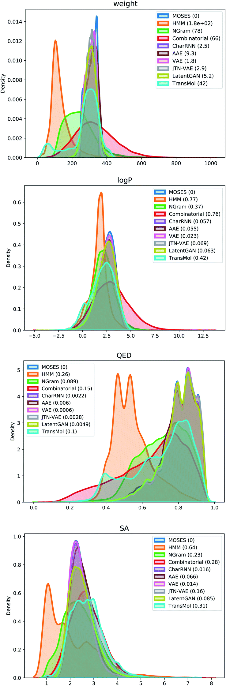
Fig. 5 demonstrates distribution plots of the baselines and Transmol output compared to the test set. The distribution plots are similar to the histograms, but instead of showing discrete bins, the distribution plot smoothes the observations using a Gaussian kernel. The distribution plots compare four molecular properties: molecular weight (MW), octanol–water partition coefficient (logP), quantitative estimation of drug-likeness (QED), and synthetic accessibility score (SA). To quantify the distance between the test set and the generated set the Wasserstein-1 distance was used (value in brackets). The results show that Transmol has a matching SA score, or better than the original distribution while having a higher variance in other metrics. It shows that Transmol is not as close to the testing set distribution as other neural algorithms, implying a higher diversity, but it is not as far from it as some simpler, combinatorial baselines.

Fig. 5 Plots of Wasserstein-1 distance between distributions of molecules in the generated and test sets.

4.1.2 Analyzing Transmol with medicinal chemistry filters. To provide more comparisons we also have filtered molecules by using some heuristics that are commonly employed in drug development. These types of filters have been empirically devised using a database of drug suitable compounds. For this comparison, we have used the Lipinski rule of 5,⁷² Ghose,⁷³ Veber,⁷⁴ rule of 3,⁷⁵ and REOS⁷⁶ filters (see ESI† for specific constrains of each filter). All properties for constraint testing were computed using the RDKit library.⁶⁷ Fig. 6 demonstrates proportions of molecules that satisfy each rule.

Fig. 6 Proportions of molecules that satisfy five different medicinal chemistry filters.

As can be seen in Fig. 6 Transmol has the highest proportion of molecules that satisfy the rule of 3 among the neural baselines. In addition, among non-neural algorithms, Transmol has the highest proportion of molecules that satisfy the Ghose filter and REOS.

4.2 Transmol validation via the recreation of known vitamin D receptor ligands

In order to show the applicability of our model to a real protein target, VDR has been chosen due to its importance in various physiological processes and the fact that there are many known VDR ligands that can be readily retrieved from established databases. For this purpose a small subset of known VDR ligands have been chosen from the ZINC database to fine tune our model and then use Transmol to recover as many known ligands as possible.

Across the 10 sampling cycles our algorithm was able to recover 27 known VDR ligands from the employed ZINC dataset. Given that the ZINC database allowed us to extract the structures of 210 VDR ligands with stripped stereoisomeric information, we have recovered 12.9% of all structures within this dataset.

The recovery process was performed 10 times where VDR ligands were re-sampled into the training and test set randomly. The minimum and maximum number of recovered molecules per cycle were 1 and 9, respectively. On average the algorithm generated 4.1 molecules per sampling cycle.

Of the 27 recovered molecules 56% were secosteroid backbone (Fig. 3A) and the rest non-steroidal VD analogues (Fig. 3C). The algorithm did not recover any steroid backbone based analogs (Fig. 3B). It is remarkable that the algorithm was able to recover the natural ligand 1,25D₃ (Fig. 3A), as well as the first non-steroidal 3,3-diphenylpentane analog YR301 (Fig. 3C). It should be noted that the group of non-steroidal ligand contains two subgroups, the first are cannonical ligands that bind to the ligand-binding pocket of VDR as secosteroid and steroid acids. The second group contains possible coactivator mimetics that irreversible compete with coactivator interaction on the surface of VDR. Thus, the above described approach constitutes a newly established benchmark for validation of generative algorithms, which examines how well the model can recreate the known ligands to a particular biological target.

4.3 Exploring chemical space using two-seeds approach

In this section, we discuss the generation of diverse libraries using two seed molecules. Fig. 7 gives a pictorial overview of the sampling procedure. Using the Transmol encoder network we encode two molecules, thus obtaining their latent representation. Then, we average them to get a latent vector z₁₂ that is located between the two latent vectors z₁ and z₂. Then, we sample the decoder using vector z₁₂. To increase the chance of sampling from the populated latent space we enumerate the SMILES representations of the seed molecules and construct pairs. This twist increases the chances of obtaining valid SMILES strings when sampling the middle point.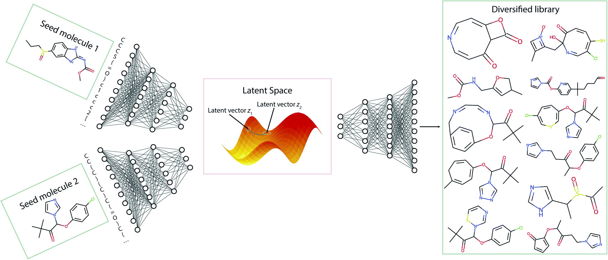

Fig. 7 The general pipeline of the sampling process for the two-seeds approach.

While the basic case of getting vector z₁₂ through averaging the individual vectors, a more general approach would be computation of weighted sum. In the default case the weights of the vectors z₁ and z₂ are chosen to be 0.5. However, other valid weight combinations can also be used to navigate the latent space. We have noticed that when the weights of both vectors are close to 0.5 the algorithm tends to return only very simple molecules with low molecular weight. The above is especially true when both seed molecules have a molecular weight of more than 250 and contain more than 15 atoms (except hydrogen) meaning that their SMILES strings are relatively long. Therefore, we have varied the α parameter of the reward function of the beam search to adjust the length of the decoded SMILES strings and as a result the complexity of the resulting molecule. On the other hand when the α parameter is set too big the algorithm may return only a limited number of molecules. Thus, to create enough molecules of larger size and increased complexity, different combinations of weight distribution and the sampling reward parameter α can be tested. Overall, the possibility to vary the seeds' weight distributions along with the sampling reward parameter α provides a viable mean of traversal across molecular space (see SI for specific comparisons). Of course, not all the generated structures are stable and/or synthesizable. Nonetheless, they may still be used as inspirational ligands for molecular docking.

Fig. 8 illustrates how molecular sampling from the latent distribution using two seed molecules can help with expanding the scaffold diversity. The resulting molecular library demonstrates a diversity of structural features that would be unattainable through simple fragment substitution or through the application of the alternative one-seed approach.

Fig. 8 Expanding scaffold diversity with the two-seeds approach.

Both one-seed and two-seeds modes of Transmol are incorporated into the cheml.io⁵⁵ website as one of the methods that allows the generation of molecules on demand. For the two-seed approach, the user can specify both seeds, a weighting distribution between them and the sampling reward parameter α that influences the length of the decoded SMILES string.

5 Conclusion

In summary, we have successfully adopted a recent deep learning framework to the task of molecular generation using attention mechanisms. Upon implementation, we have benchmarked the resulting Transmol method utilizing MOSES, a benchmark introduced for the comparison of generative algorithms. Our approach outperformed state-of-the-art generative machine learning frameworks for the internal diversity (IntDiv₁ and InDiv₂) core MOSES metric. Besides, we were able to incorporate two distinct modes of molecular generation within a single generative model. The first one-seed input-guided approach appears to be instrumental for the cases that require targeted generation of focused libraries composed of close analogues of the seed structure. The second two-seed diversity-driven approach succeeds to generate molecules that resemble both seeds and is thus attractive for the tasks that require chemical space exploration. In addition, we have validated the Transmol algorithm through the recreation of known VDR ligands. This type of bench-marking represents a viable option for expanding current validation tools for in silico molecular generation and propose it to be performed for all new generative algorithms. Furthermore, an analogous workflow can be utilized in drug discovery & development to obtain potential novel biologically active hit compounds and we are currently working in this direction. Finally, we have incorporated the Transmol algorithm into our recently launched cheML.io web database of ML-generated molecules as a second generation on-demand method.

Conflicts of interest

There are no conflicts to declare.

Acknowledgements

The co-authors would like to acknowledge the support of Nazarbayev University Faculty-Development Competitive Research Grants Program to SF and FM (240919FD3926, 110119FD4520) and the support of NPO Young Researchers Alliance and Nazarbayev University Corporate Fund “Social Development Fund” for grant under their Fostering Research and Innovation Potential Program.

Notes and references

1. J.-L. Reymond, Acc. Chem. Res., 2015, 48, 722.
2. E. Lin, C.-H. Lin and H.-Y. Lane, Molecules, 2020, 25, 3250.
3. D. V. Green, in ACS Symposium Series, ed. E. O. Pyzer-Knapp and T. Laino, American Chemical Society, Washington, DC, 2019, vol. 1326, p. 81.
4. P. Schneider, W. P. Walters, A. T. Plowright, N. Sieroka, J. Listgarten, R. A. Goodnow, J. Fisher, J. M. Jansen, J. S. Duca, T. S. Rush, M. Zentgraf, J. E. Hill, E. Krutoholow, M. Kohler, J. Blaney, K. Funatsu, C. Luebkemann and G. Schneider, Nat. Rev. Drug Discovery, 2019, 19, 353.
5. P. B. Jørgensen, M. N. Schmidt and O. Winther, Mol. Inf., 2018, 37, 1700133.
6. A. Zhavoronkov, Q. Vanhaelen and T. I. Oprea, Clin. Pharmacol. Ther., 2020, 107, 780.
7. A. S. Alshehri, R. Gani and F. You, Comput. Chem. Eng., 2020, 141, 107005.
8. Q. Vanhaelen, Y.-C. Lin and A. Zhavoronkov, ACS Med. Chem. Lett., 2020, 11, 1496.
9. S. Y. Al-nami, E. Aljuhani, I. Althagafi, H. M. Abumelha, T. M. Bawazeer, A. M. Al-Solimy, Z. A. Al-Ahmed, F. Al-Zahrani and N. El-Metwaly, Arabian J. Sci. Eng., 2021, 46, 365.
10. P. C. D. Hawkins, J. Chem. Inf. Model., 2017, 57, 1747.
11. S. Das, S. Sarmah, S. Lyndem and A. Singha Roy, J. Biomol. Struct. Dyn., 2021, 39(9), 3347.
12. N. S. Pagadala, K. Syed and J. Tuszynski, Biophys. Rev., 2017, 9, 91.
13. M. Hartenfeller and G. Schneider, Wiley Interdiscip. Rev. Comput. Mol. Sci., 2011, 1, 742–759.
14. H.-J. Böhm, J. Comput.-Aided Mol. Des., 1992, 6, 61.
15. V. J. Gillet, W. Newell, P. Mata, G. Myatt, S. Sike, Z. Zsoldos and A. P. Johnson, J. Chem. Inf. Model., 1994, 34, 207.
16. K. Kawai, N. Nagata and Y. Takahashi, J. Chem. Inf. Model., 2014, 54, 49.
17. H. Chen, O. Engkvist, Y. Wang, M. Olivecrona and T. Blaschke, Drug Discovery Today, 2018, 23, 1241.
18. G. Hessler and K.-H. Baringhaus, Molecules, 2018, 23, 2520.
19. M. Hartenfeller, H. Zettl, M. Walter, M. Rupp, F. Reisen, E. Proschak, S. Weggen, H. Stark and G. Schneider, PLoS Comput. Biol., 2012, 8, e1002380.
20. M. Hartenfeller, M. Eberle, P. Meier, C. Nieto-Oberhuber, K.-H. Altmann, G. Schneider, E. Jacoby and S. Renner, J. Chem. Inf. Model., 2011, 51, 3093.
21. M. H. S. Segler and M. P. Waller, Chem.–Eur. J., 2017, 23, 6118.
22. D. C. Elton, Z. Boukouvalas, M. D. Fuge and P. W. Chung, Mol. Syst. Des. Eng., 2019, 4, 828.
23. D. Xue, Y. Gong, Z. Yang, G. Chuai, S. Qu, A. Shen, J. Yu and Q. Liu, Wiley Interdiscip. Rev.: Comput. Mol. Sci., 2018, 9, e1395.
24. N. Brown, P. Ertl, R. Lewis, T. Luksch, D. Reker and N. Schneider, J. Comput.-Aided Mol. Des., 2020, 34, 709.
25. K. Hansen, F. Biegler, R. Ramakrishnan, W. Pronobis, O. A. von Lilienfeld, K.-R. Müller and A. Tkatchenko, J. Phys. Chem. Lett., 2015, 6, 2326.
26. K. Hansen, G. Montavon, F. Biegler, S. Fazli, M. Rupp, M. Scheffler, O. A. Von Lilienfeld, A. Tkatchenko and K.-R. Muller, J. Chem. Theory Comput., 2013, 9, 3404.
27. W. Jin, C. W. Coley, R. Barzilay and T. Jaakkola, Proceedings of the 31st International Conference on Neural Information Processing Systems, Red Hook, NY, USA, 2017, p. 2604.
28. B. Sanchez-Lengeling and A. Aspuru-Guzik, Science, 2018, 361, 360.
29. G. L. Guimaraes, B. Sanchez-Lengeling, C. Outeiral, P. L. C. Farias and A. Aspuru-Guzik, arXiv, 2018, preprint, arXiv:1705.10843v3, https://arxiv.org/abs/1705.10843v3.
30. B. Sanchez-Lengeling, C. Outeiral, G. L. Guimaraes and A. Aspuru-Guzik, ChemRxiv, 2017 DOI:10.26434/chemrxiv.5309668.v3.
31. S. Harel and K. Radinsky, Proceedings of the 24th ACM SIGKDD International Conference on Knowledge Discovery & Data Mining - KDD ’18, London, United Kingdom, 2018, p. 331.
32. R. Gómez-Bombarelli, J. N. Wei, D. Duvenaud, J. M. Hernández-Lobato, B. Sánchez-Lengeling, D. Sheberla, J. Aguilera-Iparraguirre, T. D. Hirzel, R. P. Adams and A. Aspuru-Guzik, ACS Cent. Sci., 2018, 4, 268.
33. M. J. Kusner, B. Paige and J. M. Hernández-Lobato, Proceedings of the 34th International Conference on Machine Learning-Volume 70, 2017, p. 1945.
34. J. Lim, S. Ryu, J. W. Kim and W. Y. Kim, J. Cheminf., 2018, 10, 31.
35. M. H. S. Segler, T. Kogej, C. Tyrchan and M. P. Waller, ACS Cent. Sci., 2018, 4, 120.
36. W. Jin, R. Barzilay and T. Jaakkola, Proceedings of the 35th International Conference on Machine Learning, Stockholmsmässan, Stockholm Sweden, 2018, p. 2323.
37. J.-Y. Zhu, T. Park, P. Isola and A. A. Efros, 2017 IEEE International Conference On Computer Vision, ICCV, 2017, p. 2242.
38. Ł. Maziarka, A. Pocha, J. Kaczmarczyk, K. Rataj and M. Warchoł, Artificial Neural Networks and Machine Learning – ICANN 2019, Workshop and Special Sessions, Cham, 2019, p. 810.
39. S. Kang and K. Cho, J. Chem. Inf. Model., 2019, 59, 43.
40. W. Jin, R. Barzilay and T. Jaakkola, arXiv:2002.03230 [cs, stat , 2020.
41. T. Blaschke, O. Engkvist, J. Bajorath and H. Chen, J. Cheminf., 2020, 12, 68.
42. S. Wu, Y. Kondo, M.-a. Kakimoto, B. Yang, H. Yamada, I. Kuwajima, G. Lambard, K. Hongo, Y. Xu, J. Shiomi, C. Schick, J. Morikawa and R. Yoshida, npj Comput. Mater., 2019, 5, 66.
43. C. Grebner, H. Matter, A. T. Plowright and G. Hessler, J. Med. Chem., 2020, 63, 8809.
44. E. Putin, A. Asadulaev, Q. Vanhaelen, Y. Ivanenkov, A. V. Aladinskaya, A. Aliper and A. Zhavoronkov, Mol. Biopharm., 2018, 15, 4386.
45. E. Putin, A. Asadulaev, Y. Ivanenkov, V. Aladinskiy, B. Sanchez-Lengeling, A. Aspuru-Guzik and A. Zhavoronkov, J. Chem. Inf. Model., 2018, 58, 1194.
46. O. Méndez-Lucio, B. Baillif, D.-A. Clevert, D. Rouquié and J. Wichard, Nat. Commun., 2020, 11, 10.
47. M. Skalic, J. Jiménez Luna, D. Sabbadin and G. De Fabritiis, J. Chem. Inf. Model., 2019, 1205.
48. G. Chen, Z. Shen, A. Iyer, U. F. Ghumman, S. Tang, J. Bi, W. Chen and Y. Li, Polymers, 2020, 12, 163.
49. D. Weininger, J. Chem. Inf. Model., 1988, 28, 31.
50. I. Sutskever, O. Vinyals and Q. V. Le, in Proceedings of the 27th International Conference on Neural Information Processing Systems - Volume 2, ed. Z. Ghahramani, M. Welling, C. Cortes, N. D. Lawrence and K. Q. Weinberger, MIT Press, Cambridge, MA, USA, 2014, p. 3104.
51. I. J. Goodfellow, J. Pouget-Abadie, M. Mirza, B. Xu, D. Warde-Farley, S. Ozair, A. Courville and Y. Bengio, in Proceedings of the 27th International Conference on Neural Information Processing Systems - Volume 2, ed. Z. Ghahramani, M. Welling, C. Cortes, N. D. Lawrence and K. Q. Weinberger, MIT Press, Cambridge, MA, USA, 2014, p. 2672.
52. Y. Le Cun and F. Fogelman-Soulié, Intellectica, 1987, 1, 114.
53. D. E. Rumelhart, G. E. Hinton and R. J. Williams, Nature, 1986, 323, 533.
54. A. Gupta, A. T. Müller, B. J. H. Huisman, J. A. Fuchs, P. Schneider and G. Schneider, Mol. Inf., 2018, 37, 1700111.
55. R. Zhumagambetov, D. Kazbek, M. Shakipov, D. Maksut, V. A. Peshkov and S. Fazli, RSC Adv., 2020, 10, 45189.
56. D. Polykovskiy, A. Zhebrak, B. Sanchez-Lengeling, S. Golovanov, O. Tatanov, S. Belyaev, R. Kurbanov, A. Artamonov, V. Aladinskiy, M. Veselov, A. Kadurin, S. Johansson, H. Chen, S. Nikolenko, A. Aspuru-Guzik and A. Zhavoronkov, arXiv, 2020, preprint, arXiv:1811.12823v5, https://arxiv.org/abs/1811.12823v5.
57. J. Arús-Pous, S. V. Johansson, O. Prykhodko, E. J. Bjerrum, C. Tyrchan, J.-L. Reymond, H. Chen and O. Engkvist, J. Cheminf., 2019, 11, 71.
58. A. Vaswani, N. Shazeer, N. Parmar, J. Uszkoreit, L. Jones, A. N. Gomez, u. Kaiser and I. Polosukhin, Proceedings of the 31st International Conference on Neural Information Processing Systems, Red Hook, NY, USA, 2017, p. 6000.
59. Transmol Gitlab page, https://gitlab.com/cheml.io/public/transmol, accessed July 2021.
60. The Annotated Transformer, https://nlp.seas.harvard.edu/2018/04/03/attention.html, accessed January 2021.
61. K. Preuer, P. Renz, T. Unterthiner, S. Hochreiter and G. Klambauer, J. Chem. Inf. Model., 2018, 58, 1736.
62. A. Kadurin, A. Aliper, A. Kazennov, P. Mamoshina, Q. Vanhaelen, K. Khrabrov and A. Zhavoronkov, Oncotarget, 2017, 8, 10883.
63. T. Blaschke, M. Olivecrona, O. Engkvist, J. Bajorath and H. Chen, Mol. Inf., 2018, 37, 1700123.
64. D. Polykovskiy, A. Zhebrak, D. Vetrov, Y. Ivanenkov, V. Aladinskiy, P. Mamoshina, M. Bozdaganyan, A. Aliper, A. Zhavoronkov and A. Kadurin, Mol. Biopharm., 2018, 15, 4398.
65. O. Prykhodko, S. V. Johansson, P.-C. Kotsias, J. Arús-Pous, E. J. Bjerrum, O. Engkvist and H. Chen, J. Cheminf., 2019, 11, 74.
66. J. Degen, C. Wegscheid-Gerlach, A. Zaliani and M. Rarey, ChemMedChem, 2008, 3, 1503–1507.
67. RDKit, Open-source cheminformatics, http://www.rdkit.org, accessed September 2020.
68. R. F. Chun, P. T. Liu, R. L. Modlin, J. S. Adams and M. Hewison, Front. Physiol., 2014, 5, 151.
69. A. Verstuyf, G. Carmeliet, R. Bouillon and C. Mathieu, Kidney Int., 2010, 78, 140.
70. R. Bouillon, W. H. Okamura and A. W. Norman, Endocr. Rev., 1995, 16, 200.
71. T. Sterling and J. J. Irwin, J. Chem. Inf. Model., 2015, 55, 2324.
72. C. A. Lipinski, F. Lombardo, B. W. Dominy and P. J. Feeney, Adv. Drug Delivery Rev., 1997, 23, 3.
73. A. K. Ghose, V. N. Viswanadhan and J. J. Wendoloski, J. Comb. Chem., 1999, 1, 55.
74. D. F. Veber, S. R. Johnson, H.-Y. Cheng, B. R. Smith, K. W. Ward and K. D. Kopple, J. Med. Chem., 2002, 45, 2615.
75. M. Congreve, R. Carr, C. Murray and H. Jhoti, Drug Discovery Today, 2003, 8, 876.
76. W. P. Walters and M. Namchuk, Nat. Rev. Drug Discovery, 2003, 2, 259.

---

Footnote

† Electronic supplementary information (ESI) available. See DOI: 10.1039/d1ra03086h

---