
 Open Access Article
 This Open Access Article is licensed under a Creative Commons Attribution-Non Commercial 3.0 Unported Licence
Advanced analysis of magnetic nanoflower measurements to leverage their use in biomedicine
Augustas
Karpavičius†
a,
Annelies
Coene†
 bc,
Philipp
Bender‡
d and
Jonathan
Leliaert
*a
bc,
Philipp
Bender‡
d and
Jonathan
Leliaert
*a
aDepartment of Solid State Sciences, Ghent University, Ghent, Belgium. E-mail: jonathan.leliaert@ugent.be
bDepartment of Electromechanical, Systems and Metal Engineering, Ghent University, Zwijnaarde, Belgium
cCancer Research Institute Ghent, Ghent, Belgium
dDepartment of Physics and Materials Science, University of Luxembourg, Luxembourg, Grand Duchy of Luxembourg
First published on 8th February 2021
Abstract
Magnetic nanoparticles are an important asset in many biomedical applications ranging from the local heating of tumours to targeted drug delivery towards diseased sites. Recently, magnetic nanoflowers showed a remarkable heating performance in hyperthermia experiments thanks to their complex structure leading to a broad range of magnetic dynamics. To grasp their full potential and to better understand the origin of this unexpected heating performance, we propose the use of Kaczmarz' algorithm in interpreting magnetic characterisation measurements. It has the advantage that no a priori assumptions need to be made on the particle size distribution, contrasting current magnetic interpretation methods that often assume a lognormal size distribution. Both approaches are compared on DC magnetometry, magnetorelaxometry and AC susceptibility characterisation measurements of the nanoflowers. We report that the lognormal distribution parameters vary significantly between data sets, whereas Kaczmarz' approach achieves a consistent and accurate characterisation for all measurement sets. Additionally, we introduce a methodology to use Kaczmarz' approach on distinct measurement data sets simultaneously. It has the advantage that the strengths of the individual characterisation techniques are combined and their weaknesses reduced, further improving characterisation accuracy. Our findings are important for biomedical applications as Kaczmarz' algorithm allows to pinpoint multiple, smaller peaks in the nanostructure's size distribution compared to the monomodal lognormal distribution. The smaller peaks permit to fine-tune biomedical applications with respect to these peaks to e.g. boost heating or to reduce blurring effects in images. Furthermore, the Kaczmarz algorithm allows for a standardised data analysis for a broad range of magnetic nanoparticle samples. Thus, our approach can improve the safety and efficiency of biomedical applications of magnetic nanoparticles, paving the way towards their clinical use.
1 Introduction
Due to their ubiquitous use in biomedicine, magnetic nanostructures have become indispensable tools in life science applications.1,2 For instance, these structures can locally heat up cancerous tissues in cancer hyperthermia treatments,3,4 or act as medicine carriers that can be magnetically guided towards diseased sites in drug targeting.5 Because of the local nature of these therapies, less systemic side effects and a higher therapeutic efficacy are achieved as compared to traditional treatments. Next to their success in various therapies, they are also valuable for many diagnostic applications such as high-throughput screening platforms and immunoassays that exploit their sensitivity in finding and determining the concentration of various biological entities. Also in magnetofection applications do they offer a sublime performance in passing genes through cellular boundaries.6,7 Given the fact that the human body is virtually devoid of ferromagnetic materials and that magnetic signals are not attenuated by it, a range of magnetic imaging techniques exist that directly capture the nanostructures' behaviour in terms of location and concentration. Among these techniques, Magnetic Particle Imaging (MPI)8,9 is the most known and matured towards clinical applications such as vascular perfusion imaging,10 stem cell tracking11 and image-guided hyperthermia.12 Nevertheless, other still-to-mature nanoparticle imaging techniques such as magnetorelaxometry imaging (MRXi)13,14 and magnetic susceptibility imaging (MSI)15,16 have a promising future ahead. It is also possible to increase the sensitivity and/or resolution of established diagnostic imaging techniques by indirectly measuring the impact of the particles' magnetic fields on the imaging signal. A prime example thereof is the use of magnetic nanoparticles as contrast agents in magnetic resonance imaging (MRI).17,18Previous applications each set different requirements on the nanostructures resulting in the development of a large range of nanoparticles types. For some applications, like MPI, there exist clear requirements, based on theory, that work well in practise to achieve good performance.19 In this case, for instance, the optimal particles have a size that is as large as possible, while still maintaining a relaxation time lower than the inverse of the used MPI frequency to resolve blurring issues in the image. Additionally the size distribution should be as monodisperse as possible. In magnetic particle hyperthermia,20 however, the situation is much less clear, because uniformly magnetised particles do not necessarily offer the best performance. Instead, there are indications that coherent reversal processes perform worse than more complex dynamical processes,20,21 which means that the suitability for hyperthermia strongly depends on the microscopic details of the particles. Unfortunately, there are no straightforward theories that can make predictions in this regime, and a computationally intensive micromagnetic approach22 is necessary. However, for such an approach to give practical results, the simulations should mimic the real particle ensemble including the inter-particle variability in size, shape and material parameters as closely as possible, which still lies beyond today's capabilities.23
Given the complexity of this problem, it is not surprising that also experimental data on different particle types and sizes are not converging.24,25 Moreover, possible magnetic interactions between the magnetic cores occur that manifest themselves differently depending on the type of applied magnetic fields and the surroundings of the particles. Next to this, when the particles are injected in the body also interactions with biological entities occur. These types of interactions were shown to have a significant impact on the particles' heating performance.26–29 However, among the different particle types that are being investigated, one type consistently stands out with excellent performance:30–32 magnetic nanoflowers.33 These are multi-core particles with an irregular shape, consisting of a large number of small crystallites.34 The collective properties of the interacting crystallites result in different magnetic behaviour than their single-core counterparts, allowing for a large magnetic moment while still maintaining faster dynamics normally associated with smaller particles. Due to their dense structure and single-domain character, nanoflowers can also be regarded as individual particles but with a very high defect-density in their nanocrystalline structure. Together with other large but defect-rich iron oxide nanoparticles, their excellent performance in various biomedical applications recently motivated a new design avenue for the synthesis of magnetic nanoparticles, namely defect-engineering.35
To understand why certain nanostructures such as nanoflowers and other defect-rich particles36,37 achieve such powerful heating, or why a certain nanostructure is an optimal imaging tracer, and to ensure a safe and reliable operation of previously mentioned applications, an accurate particle characterisation of e.g. the particle core and hydrodynamic size distribution is of paramount importance. Several optical and magnetic characterisation methods, each with their unique advantages and drawbacks, exist that try to tackle this challenge.38
One common optical technique for determining the hydrodynamic particle size is dynamic light scattering (DLS). The main disadvantage of this technique is that the signal scales with the square of the particle volume, and a few large particles can therefore overshadow the details of the smaller particles in the sample. A more accurate method is transmission electron microscopy (TEM) and its high resolution variant (HRTEM), which also gives access to the core sizes. As compared to other methods, this has the disadvantage that it is relatively slow due to the need for sample preparation (which potentially affects the particle clustering). The ability to investigate individual particles also comes with the downside that several measurements are required to gather sufficient statistics to reliably describe samples containing billions of particles. To circumvent this problem, one can resort to X-ray based techniques like X-ray diffraction (XRD) and small-angle X-ray scattering39 (SAXS) which measure the particle structures, averaged out over the entire ensemble.
Similar to SAXS, also small-angle neutron scattering (SANS) can be used to determine the structural properties (i.e. the average size, shape and configuration) of nanoparticle ensembles.32,40 Additionally, SANS allows one to access the internal magnetisation profile,41,42 which renders it in general as an ideal technique to characterise complex nanostructured magnetic samples.43 However, SANS is a highly complex technique which can be only performed at large-scale facilities whose access requires a long proposal application process, making it impractical as a day-to-day characterisation method.
Next to these optical methods, there exist several magnetic characterisation methods, which probe the magnetic properties of the particles, and which we will focus on in this paper. Three commonly used methods are DC magnetometry (DCM), magnetorelaxometry (MRX) and AC-susceptibility (ACS). DCM is the oldest of these methods, and interprets the magnetisation measured as function of an externally applied static magnetic field.44 This method is complementary to MRX and ACS as it is an equilibrium measurement. This contrasts MRX and ACS which probe the dynamic response of the particles. In case of MRX, the relaxation towards the paramagnetic state is measured after the application of a magnetic field pulse that temporarily magnetises the sample,45 whereas in ACS46 the particles are subject to a continuously applied sinusoidally varying magnetic field with low amplitude. The physical quantity derived by MRX and ACS is the relaxation time, which is then interpreted in terms of a core and/or hydrodynamic size of the particles. This translation between relaxation times and particle sizes is based on the assumption that the particles are single domain, non-interacting spheres. Additionally, to keep this problem tractable,47 a lognormal size distribution is often assumed.48 In practice, it is not feasible to consider a (correlated) lognormal distribution for both the particle core sizes as well as their hydrodynamic size. Therefore often additional assumptions are made such as a fixed particle shell size or lognormal distribution parameters are extracted from characterisation measurements under varying particle conditions.27,49,50 It is clear that these assumptions are difficult to reconcile with the specifics of multicore particles or nanoflowers, which are irregularly shaped particles consisting of several core crystallites.
Moreover, because different magnetic characterisation measurements probe different magnetisation dynamics of the nanostructures in a complementary way, an advantage is to be expected by combining multiple measurements to extract more accurate results. Yet, this combined analysis of multiple characterisation measurements remains almost unexplored. Only in pulsed MPI, this aspect has been recently exploited by introducing a pulsed magnetic field in the imaging field sequence of MPI.51 This resulted in an improved resolution as compared to traditional MPI. In line with this result, we recently improved the characterisation performance of MRX by employing a pulsed sinusoidal or circular field instead of a constant pulse to increase the information content in the measurement data.52 These results indicate that an additional characterisation improvement is indeed achievable by combining measurement sets.
In this paper, we will investigate how nanoflowers can be accurately characterised by interpreting measurement data using Kaczmarz' algorithm,53 which is an approach that does not require one to make any a priori assumptions on the size distribution. We will interpret four data sets, obtained using DCM, MRX (on both immobilised and suspended nanoparticles) and ACS. Our results will be compared with the typical approach which is based on the assumption of a lognormal size distribution and with other results obtained with optical characterisation techniques (DLS, XRD, TEM and HRTEM). Additionally, building on the approaches presented in ref. 32 and 54, we are the first to simultaneously exploit the information present in different characterisation measurements using Kaczmarz' method for an improved characterisation. Finally, we discuss the implications of our results for biomedical applications.
2 Methods
2.1 Sample information
Our analysis is performed on the NF-3 sample of which the synthesis and the measurement of magnetic properties are presented in Gavilán et al.552.2 Particle characterisation methods
We analyse data obtained from the sample using three different experimental magnetic nanoparticle characterisation techniques, namely DC magnetometry (DCM), magnetorelaxometry (MRX), and AC susceptibility (ACS). In the following sections, we detail the physical models used to interpret the measurement signal in terms of the particle properties.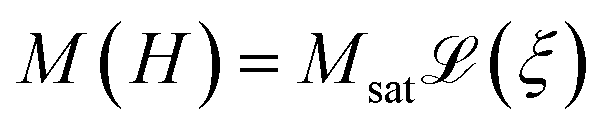 | (1) |
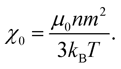
 denotes the Langevin function and Msat is the saturation magnetisation (which for our sample equals 444 kA m−1 (ref. 55))
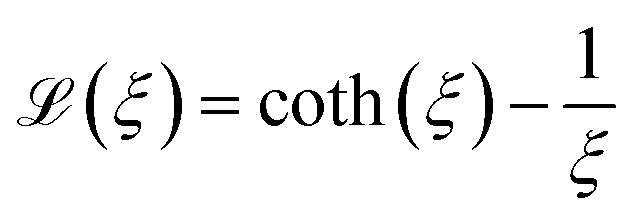 | (2) |
 has an argument, ξ, given by:
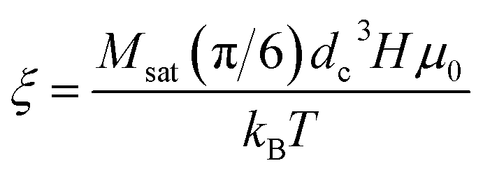 | (3) |
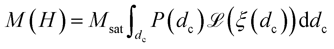
In this equation, H, denotes the magnetic field strength, μ0, the vacuum permeability, dc the nanoparticle core diameter, kB the Boltzmann constant and T the temperature. The signal corresponding to a sample with core size distribution P(dc) is then described by
 | (4) |
Note that one has to be careful about the weighting of the distribution (volume vs. number weighted). In this notation, the distribution P(dc) is volume weighted.
 | (5) |
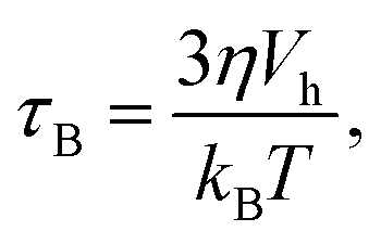
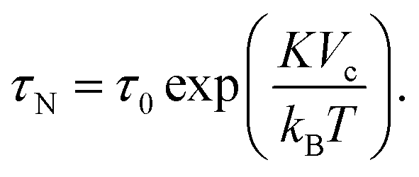
The second process is called the Néel relaxation and is caused by thermal activation, allowing the magnetic moment to jump over energy barriers, thus changing the magnetic moment direction within the particle. In this case, the motion of the magnetic moment is mechanically decoupled from the physical particle, allowing this process to also take place in immobilised particles, in which the Brownian relaxation is blocked. The rate of this relaxation process is given by the Néel relaxation time
 | (6) |
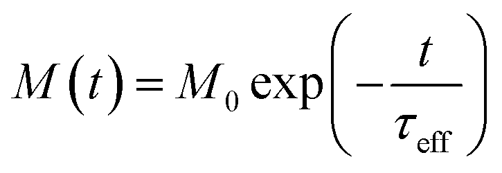
When both the Brownian and Néel relaxation processes take place simultaneously, the resulting relaxation can be described by an effective relaxation time, τeff, which is dominated by the fastest relaxation process. Thus, when we have a liquid suspension of relatively large nanoparticles, like the nanoflowers under study, we expect the Brownian relaxation to dominate the observed signal. This is corroborated by the fact that the immobilised sample relaxes on a much longer timescale than the liquid suspension, as can be seen by comparing Fig. 2a and 3a.
The relaxing magnetisation signal of a single particle is given by eqn (7),
 | (7) |
 | (8) |
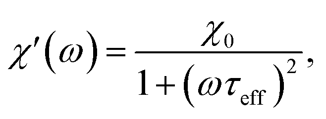
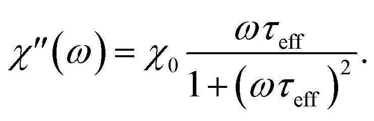
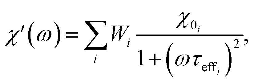
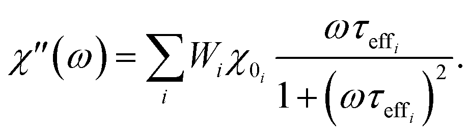
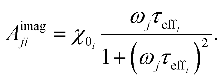
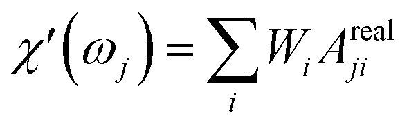
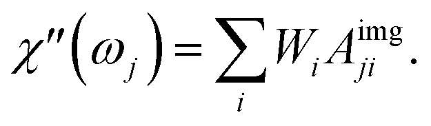
When the time scale of the measurement is longer than the relaxation time of the particle ensemble, the magnetic response will be in phase with the applied magnetic field. However, when the measurement frequency is comparable to the inverse of the relaxation time, the ensemble of particles will not be able to follow the magnetic field and an out of phase component will be present.60 In the linear response regime, the resulting amplitude and phase can be written as a complex AC susceptibility, that is described in terms of a real (χ′) and imaginary part (χ′′), linked together by eqn (9)
| χ = χ′ − iχ′′ | (9) |
The frequency (ω) dependence of the real part (χ′) is described by eqn (10)
 | (10) |
 | (11) |
 | (12) |
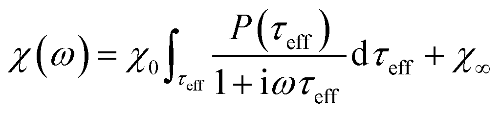
The response of the particle again is determined by an effective relaxation time τeff, comprising both Brownian and Néel relaxations, and similar as in MRX, the measured signal of a sample containing a relaxation time distribution consists of a weighted superposition of signals for each individual τeff, described by eqn (13).
 | (13) |
2.3 Size distribution reconstruction
We will use two different methods to analyse the measurement data in terms of the particle size, or relaxation time, distributions. The first method assumes that the particles are described by a lognormal distribution, whereas the second method does not make any a priori assumptions and uses Kaczmarz' method to extract the distribution. For both fitting methods we numerically consider a size range between 1 and 200 nm, in 2000 linearly spaced intervals for the size distribution of the crystallite cores dc. This is in line with HRTEM measurements of the crystallite cores.55 As the nanoflowers have an irregular shape, their hydrodynamic diameter cannot be easily represented by a dh distribution and therefore we consider a distribution of the effective relaxation times instead. Note that for these particle types the effective relaxation time corresponds to the Brownian relaxation time τB, see Section 2.2.2. Typically these have values that span several orders of magnitude, consequently, we consider an interval of 2000 logarithmically spaced relaxation times between 10−7 s and 104 s. The relaxation time values reflect how the irregular shape of the flowers varies and can retrieve possible cluster formations or particle interactions.The physical rationale behind this choice is based on two assumptions, presented in ref. 62. First, the growth of the magnetic particle volume in time t due to atomic absorption is proportional to the surface area A(t) of the nanoparticle.
Following this assumption, a differential equation can be written
 | (14) |
| V(t) ∝ t3 ⇒ dc(t) ∝ t, | (15) |
Secondly, the residence time of the particles in the active zone where they grow is lognormally distributed.
Because a lognormal distribution raised to any power remains lognormally distributed, it follows from these assumptions that both their size and relaxation time τB follow a lognormal distribution, described by eqn (16).
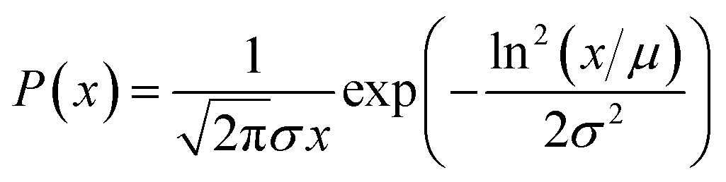 | (16) |
In this equation, x denotes either the crystallite core diameter dc or the relaxation time τB, while μ and exp(σ) can be physically interpreted as the mean diameter/relaxation time and the standard deviation of ln(x), respectively. Eqn (4), (8) and (13) can be fitted to measurement data by finding the optimal μ and σ of the distribution P(x). For the model described in eqn (13) an additional fit term χ∞ is necessary besides the μ and σ to account for the offset at high frequencies.
In order to obtain the μ and σ values that result in the best agreement with the experimental data, we will employ a nonlinear least-squares routine to fit the lognormal size distribution.
To this end, we introduce a weight vector W consisting of I = 2000 weights Wi with i = 1, …, I, each corresponding to the different particle sizes/relaxation times. W is initialised to zero.
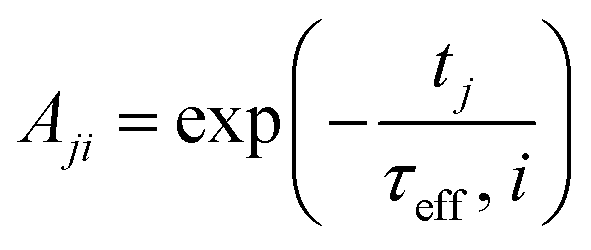
We use Kaczmarz' iterative method [eqn (17)] to update the weights vector for each iteration k, until we find a good agreement between the experimental and simulated data.
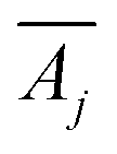
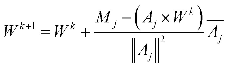 | (17) |
 denotes the transpose of this matrix, and one iteration is defined as a sweep over all rows j in a random order. In each of our fits, we employ 10
![[thin space (1/6-em)]](https://www.rsc.org/images/entities/char_2009.gif) 000 iterations. We verified that for larger iteration numbers, the error did not significantly decrease any further, and an artificial over-fitting of the data starts to take place.
000 iterations. We verified that for larger iteration numbers, the error did not significantly decrease any further, and an artificial over-fitting of the data starts to take place.
Using the matrix A, we can generate the simulated data points corresponding to the measured data points Mj by performing a matrix multiplication with the final weights vector, containing all information on the particle size distribution 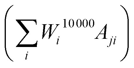 . By iteratively updating these weights, the algorithm tries to minimise the difference between the simulated and measured data, and find an accurate particle size or relaxation time distribution.
To avoid negative weights, which would correspond to unphysical effects like spontaneous remagnetisation of the particles in the case of MRX,47 we introduced a non-negativity constraint by resetting the weight to zero (Wik+1 = 0) whenever the update of the weight would result in a negative value.
The next 3 sections detail the values of the matrix A for the different measurement types.
2.3.2.1 DCM matrix. In the case of DCM, the magnetisation as a function of the applied field follows a Langevin function, whose argument depends on the particle core size. The rows of the matrix Aji, contain the theoretical field value for a given particle size dc,i in a magnetic field with strength Hj, as obtained by combining eqn (1) and (3):
 | (18) |
2.3.2.2 MRX matrix. Similarly, the MRX signal consists of a superposition of decaying exponential curves, each corresponding to different particle crystallite sizes (in case of the MRX measurement data on immobilised particles, eqn (19)) or to different relaxation time values (for the MRX measurement data on suspended particles, eqn (20)).
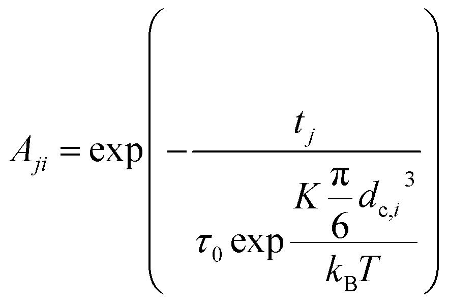 | (19) |
 | (20) |
2.3.2.3 ACS matrix. In the same manner as for magnetorelaxometry, by introducing a superposition of curves for different relaxation times and a weight vector we can rewrite the real (χ′) and imaginary (χ′′) parts of the ACS curve as
 | (21) |
 | (22) |
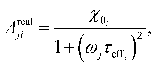 | (23) |
 | (24) |
So that the susceptibility at any frequency j is described by
 | (25) |
 | (26) |
3 Results
The results are subdivided into two sections because DC magnetometry and magnetorelaxometry of immobilised particles are mainly sensitive to the size of the individidual nanocrystallites making up the nanoflower, whereas AC suceptibility and magnetorelaxometry of suspended nanoflowers mainly give information on the hydrodynamic size of the nanoflower.3.1 Nanocrystallite size
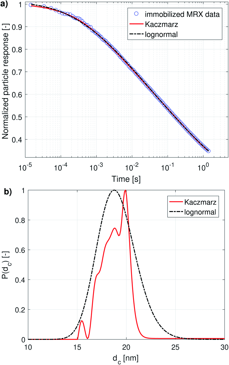
Fig. 1a and 2a show the DCM and MRX measurement data respectively, together with the best fit obtained with Kaczmarz' method and by the nonlinear least squares fit assuming a lognormal size distribution. The fitted parameters for the lognormal size distribution are given in Table 1.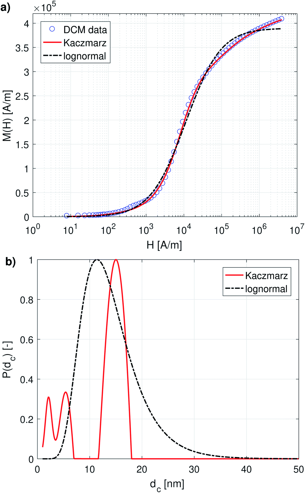 | ||
| Fig. 1 (a) DCM data with best fits obtained using a lognormal distribution and using Kaczmarz' method. (b) The obtained size distributions corresponding to the fits in panel (a). | ||
 | ||
| Fig. 2 (a) Best fit of the magnetorelaxometry measurement data of immobilised sample using a lognormal distribution and using Kaczmarz' method. (b) The obtained size distributions corresponding to the fits in panel (a). | ||
| μ (nm) | σ | |
|---|---|---|
| DCM | 13.1 | 0.37 |
| MRX (immobilised) | 18.9 | 0.10 |
Although both the lognormal fit and Kaczmarz' method are able to fit the general shape of the DCM data, the restriction of a lognormal size distribution does not allow one to find a good agreement in the entire field range. In particular, at high magnetic fields, there is a noticeable difference between the measured and fitted curve, suggesting that the real size distribution in fact is not described very well by a lognormal distribution. This contrasts the best fit obtained using Kaczmarz' method, which is in good agreement with the measurement data over the entire field range.
To gain insight into the discrepancy between both fitted curves, we turn our attention to Fig. 1b, which shows the size distributions obtained from the DCM measurements displayed in panel (a). The reconstructed size distribution using Kaczmarz' algorithm exhibits several peaks: one main peak around 16 nm, and two smaller peaks between 1 nm and 10 nm. By definition, the lognormal distribution only has one peak, and we observe that the lognormal distribution that best describes the data can not even completely envelope the multi-peak distribution obtained with Kaczmarz' method due to the restrictions on the shape of its small-particle tail. Nonetheless, to account for the small-diameter contributions, the distribution is artificially broadened. This results in a substantially shifted peak as compared to the distribution obtained with Kaczmarz' method and the appearance of a long tail beyond 20 nm, which is the main cause of the discrepancies between the experimental data and the best fit shown in Fig. 1a. As can be seen in the remainder of this section, the tail, corresponding to nanocrystallites with diameters above 20 nm, is also not observed using any of the other measurement methods such as MRX and optical alternatives.
The magnetorelaxometry measurements of the immobilised nanoparticles, shown in Fig. 2a, at first sight tell a different story. In this case, both the least squares fit using the assumption of a lognormal size distribution, as well as the Kaczmarz' fit describe the data reasonably well. The corresponding size distributions, displayed in Fig. 2b, also are in good agreement and show a large peak at 19 nm. In the case of Kaczmarz' method the peak consists of two sub-peaks at 18 and 20 nm and is preceded by a smaller peak at 15 nm. Together, these findings corroborate the main peak found in the distributions based on DCM measurements. The absence of the peaks at lower sizes is not an inconsistency between both data sets, but can be attributed to the limited sensitivity of MRX towards particles smaller than about 15 nm, corresponding to a Néel relaxation time τN ≈ 10−5 s, which is the resolution of the measurement.
We now compare these results with size estimates obtained using optical methods. Gavilán et al.55 report a total size of the nanoflowers of around 110 nm according to transmission electron microscopy (TEM), and a hydrodynamic size of about 158 nm according to dynamic light scattering (DLS), and an average crystallite size of 8 nm based on X-ray diffraction (XRD) measurements and of 4 nm using HRTEM. The main peak of the distribution obtained from DCM data is above the average crystallite size but significantly below the total nanoflower size. This indicates that the atomic moments of neighbouring crystallites are exchange coupled to some extent, resulting in effective magnetic moments for each nanoflower which are larger than the moments of the individual crystallites. However, these nanoflowers are not single-domains as was observed for example for the nanoflowers investigated in Bender et al.32 The secondary peaks observed between 1 and 10 nm in our distribution obtained from the DCM data are in good agreement with the crystallite sizes determined by XRD and HRTEM. The information on how the nanocrystallites influence each other's magnetic dynamics is also important and useful when assessing the performance of the nanostructure for different applications as it for example has an impact on the observed heating of the structure for magnetic hyperthermia experiments and on its imaging performance.63 Optical methods do not register the impact of magnetic interactions on the crystallites and hence only see the individual crystallites.
3.2 Hydrodynamic size
Magnetorelaxometry and AC susceptibility of suspended particles measure the Brownian relaxation rate of the particles, which is the velocity of their mechanical rotation in the suspension. To interpret this rotation in terms of diameters [eqn (5)] we need to rely on the assumption that the particles are spherical, which is not the case for the irregularly shaped nanoflowers. Therefore, we will present the obtained distributions as distributions of the relaxation rates instead of diameter distributions. Only when comparing the results with the ones obtained from DLS and TEM will we convert them into an effective diameter and take into account that only a very rough agreement is expected. From an application's viewpoint, the relaxation rates are also more practical to work with, because these indicate the optimal frequency that can be used in e.g. magnetic nanoparticle hyperthermia or imaging.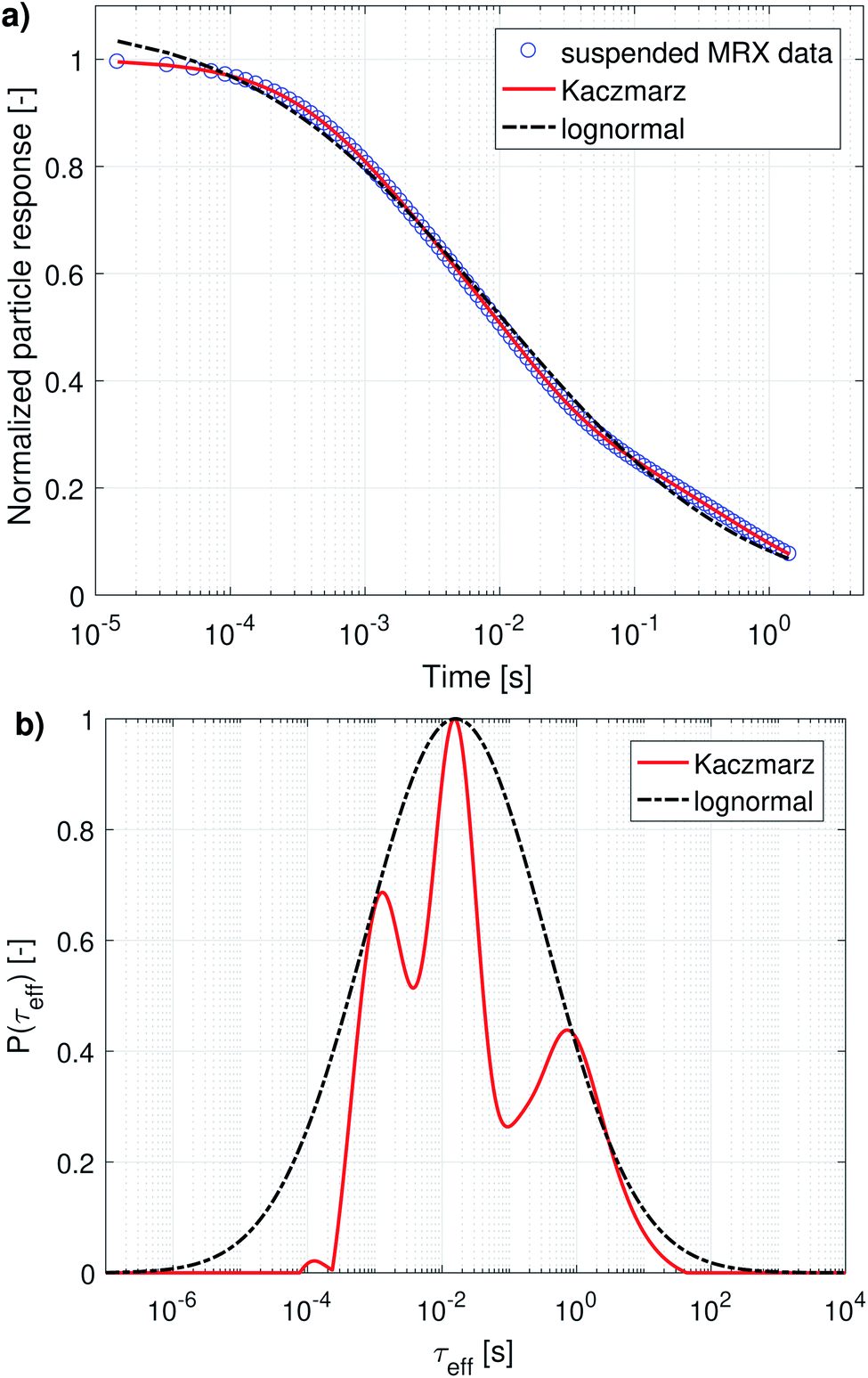 | ||
| Fig. 3 (a) Best fit of the magnetorelaxometry measurement data of suspended nanoflowers using a lognormal distribution and using Kaczmarz' method. (b) The obtained relaxation time distributions corresponding to the fits in panel (a). | ||
The distribution obtained using Kaczmarz' method consists of three distinct peaks enveloped by the lognormal distribution. The parameters of the lognormal distribution are shown in Table 2. Due to the broadness of the distribution (ranging over more than 5 orders of magnitude in relaxation times) it is not straightforward to interpret μ and σ. Although μ seems to be very large (226 s), the actual peak value is given by exp(ln(μ) − σ2) = 16 ms, and corresponds to an effective diameter of 350 nm.
| μ (s) | σ | Peak (ms) | Eff. diam. (nm) | |
|---|---|---|---|---|
| MRX | 227 | 3.09 | 16 | 348 |
| ACS (real) | 0.014 | 1.27 | 2.8 | 194 |
| ACS (imag) | 0.055 | 1.57 | 4.7 | 231 |
| ACS (both) | 0.072 | 1.64 | 5.1 | 237 |
| Combined | 3.125 | 2.19 | 26 | 408 |
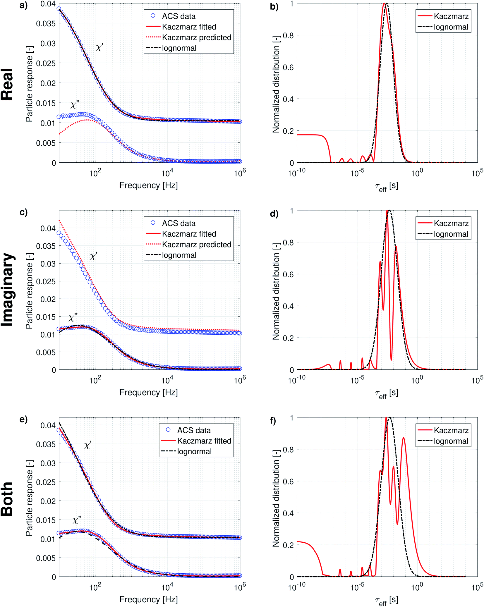 | ||
| Fig. 4 Best fit of the AC-susceptibility measurement data of suspended nanoflowers using a lognormal distribution and using Kaczmarz' method, based on (a) the real part of the data, (c) the imaginary part of the data, (e) both parts of the data set. Panels (b, d and f) show the obtained relaxation time distributions corresponding to the fits in panels (a, c and e), respectively. | ||
The complex AC-susceptibility consists of a real part [the upper blue data points in Fig. 4a, c and e] and an imaginary part [the lower blue data points in Fig. 4a, c and e]. In our analysis, we will first analyse the real and imaginary part individually [results shown in panels (a–d)], and subsequently analyse both parts simultaneously [results shown in panels (e and f)].
In panels (a and c) the black dash-dotted lines correspond to the lognormal distribution that best fits the real and imaginary part of our data set, respectively. The corresponding parameters μ and σ are shown in Table 2 and show that the obtained peaks in relaxation time lie at 2.8 ms and 4.7 ms, corresponding to an effective diameter of 194 nm and 231 nm.
The full red lines in the same figures indicate the fits obtained using Kaczmarz' method and show that an excellent agreement with both data sets is obtained. The dotted red lines correspond to the predicted imaginary [panel (a)] or real part [panel (c)] signal derived from the found distributions by fitting to the real/imaginary part of the data using Kaczmarz' method. Similar deviations were found when using the distribution obtained through fitting of a lognormal, but these were omitted from the figures for clarity reasons. Interestingly, it seems as if the real and imaginary data are not mutually consistent as the best fit with one of the data sets results in a rather poor fit to the other data.
This picture is corroborated by the best fit obtained from both data sets simultaneously [as shown in panel (e)], in which an overshoot of the real data and undershoot of the imaginary data is visible at low frequencies for the lognormal fit, and also (to a lesser extent) in the fit obtained using Kaczmarz' method. This means that these data are not well described by eqn (9) to (12) at low frequencies. Possible explanations for this effect are that the measurement is no longer in the linear response regime at these low frequencies or that the measurement setup lacks accuracy at lower frequencies.
We leave a quantitative discussion of the peak positions in the obtained distributions shown in panels (b, d and f) for the next section. Instead we first qualitatively describe a few features visible in the reconstructed distributions: first, continuing our previous argument, the best fit of the combined real and imaginary part [panel (f)] obtained with Kaczmarz' method displays a peak at longer relaxation times than any of the peaks observed in the distributions of the individual data sets. This spurious peak therefore likely is an unphysical artefact in which the fitting algorithm numerically compensated for the limitations of the physical model or the setup at low frequencies.
Secondly, the lognormal distributions typically envelope the distributions obtained with Kaczmarz' method (except for the unphysical peak described above), but only in the real part of the data is there a good agreement between both obtained distributions. Unlike any of the other found distributions, the one retrieved from the real part of our data displays only one peak (with a broad shoulder towards longer relaxation times). We argue that this originates from the relatively featureless form of eqn (10) which at frequency f shows a convolution of all signal contributions with τeff > f. Moreover, the real part of our measurement data shows a large offset even up to the largest measured frequencies that must come from frequencies above our measurement limit of 1 MHz, see also eqn (13). Physically, these high frequency contributions stem from the magnetisation dynamics within the potential energy wells of the magnetocrystalline anisotropy (as opposed to the thermal switching between these wells) at above GHz frequencies.61 This interpretation is corroborated in the distribution found by Kaczmarz by the appearance of a plateau at very fast (<10−7 s) relaxation times in the reconstructed distribution. This contribution is implicitly accounted for in the lognormal distribution because of the additional fit parameter χ∞ in the model [see eqn (13)].
All reconstructed distributions also show a number of small peaks at fast relaxation rates, which we attribute to a small artefact in our data. The data were measured in two different frequency ranges, with two different setups: one ranging from 10 Hz to 10 kHz, and one ranging from 10 kHz to 1 MHz. Because both data sets do not perfectly match numerically, Kaczmarz' algorithm tries to compensate for this by adding these spurious peaks. We verified that these peaks were not obtained when only fitting to one frequency range of the data set.
Finally, the imaginary part of our measurement data still shows a large signal at the lowest available frequency, i.e., 10 Hz. This means that our ACS data set does not contain information of all dynamical processes present in our sample. Luckily, whereas ACS is mainly sensitive to processes displaying a fast relaxation time, MRX is more sensitive to processes which display slower relaxation times. In the next subsection we will therefore combine both data sets into one analysis before discussing the location of the obtained peaks in detail.
In order to use Kaczmarz' method on two data sets, they are combined into one array. Likewise, the two A matrices [see Section 2.3.2] are merged in a way such that the weights of the distribution, multiplied by A give rise to one single array containing both reconstructed data sets, comparable to the combined input data array. There are, however, two additional steps necessary in order to ensure a good fit. First, each of the two data sets needs to get the same weight in the reconstruction to avoid that the obtained distribution is dominated by one of the data sets. This is done by normalising each of the individual A matrices such that the sum of all elements is the same for both matrices. Next, the multiplication of the weights with A only describes the shape of the data up to a prefactor. In the individual fits, this prefactor is implicitly fitted together with the weights. In a combined fit, this is not possible, because both data sets do not necessarily display the same prefactor. We therefore add an additional step after each iteration, in which the individual measurement data sets are rescaled to the reconstructed curve, to ensure that the same weights can be used to find a good fit of both data sets simultaneously. Finally, in this case it is even more important than in the other fits that we iterate through all data points in a random order, to avoid any biases that could arise by always iterating through each complete individual data sets in the same order.
In the following, we will discuss the results of a combined fit of the MRX measurement data and the imaginary part of the ACS measurement data. We chose only to take the imaginary part of the ACS data into account because it contains, in principle, the same information as the real part, but as argued in the previous section, the real part is less sensitive, contains a high frequency offset, and seems inconsistent with the imaginary part of the data at low frequencies.
The results of this combined fit are depicted in Fig. 5 and show that both in the MRX data [panel (a)] and imaginary ACS data [panel (b)] a good fit can be obtained using Kaczmarz' method. This contrasts the best fit obtained using a lognormal distribution which displays significant deviations from both data sets.
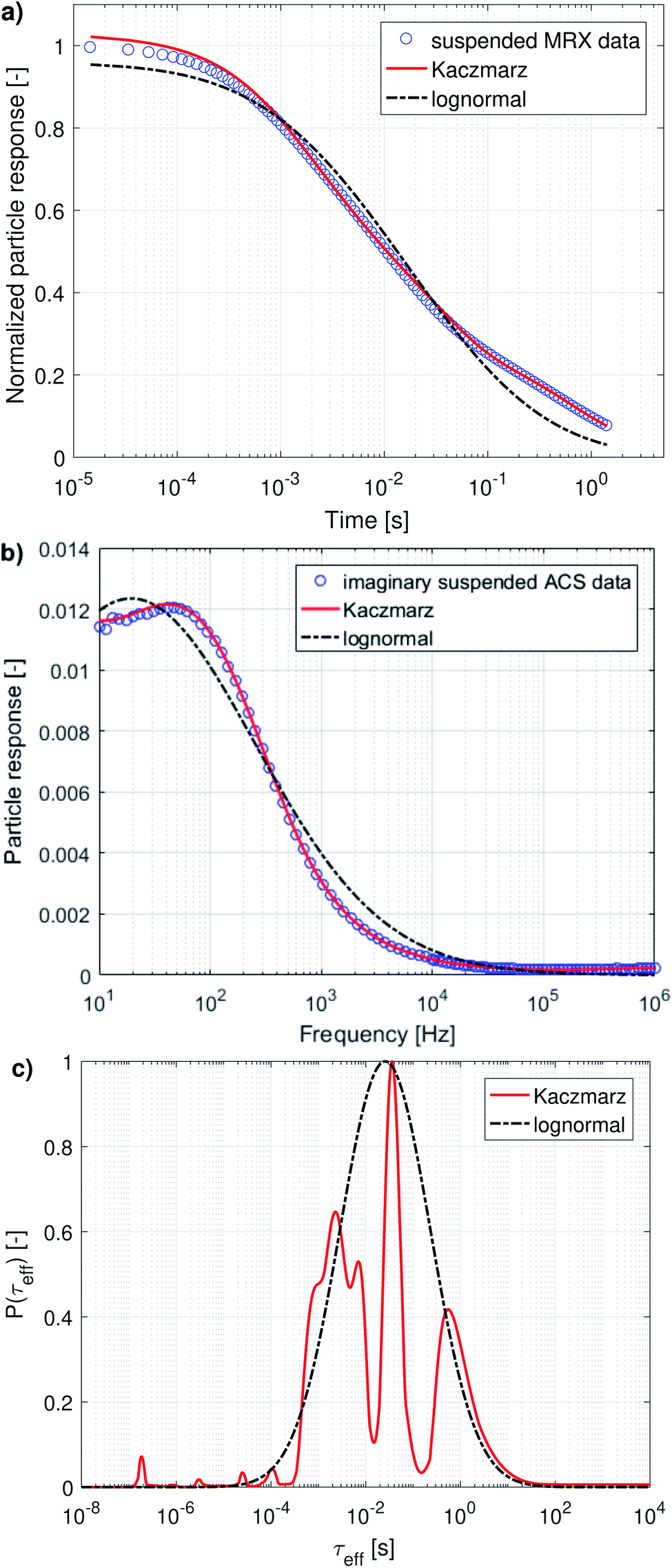 | ||
| Fig. 5 Best combined fit to (a) the magnetorelaxometry measurement data and (b) imaginary part of the AC-susceptibility measurement data of suspended nanoflowers using a lognormal distribution and using Kaczmarz' method. (c) The obtained relaxation time distributions corresponding to the fits in panel (a and b). | ||
The obtained parameters μ and σ for the fitted lognormal distribution are shown in Table 2. The lognormal distribution again roughly envelopes the distribution obtained using Kaczmarz' method and the obtained peak of the lognormal in the relaxation time (26 ms) is similar to the peak obtained from the MRX data alone (16 ms) and is significantly larger than the peak position obtained from ACS data (between 2.8 and 5.1 ms).
We will now discuss the position of the peaks in the distributions obtained with Kaczmarz' method, as collected in Table 3, in which we organised them so that peaks we identify as the same are put in the same column.
| Measurement | Peak positions (ms) | ||||
|---|---|---|---|---|---|
| a Broad shoulder next to previous peak. b Shoulder instead of peak. c Non-physical artefact. | |||||
| MRX | 1.29 | 15.26 | 728 | ||
| ACS (real) | 1.77 | ||||
| ACS (imaginary) | 0.80 | 3.02 | 16.41 | ||
| ACS (both) | 0.89b | 2.57 | 10.60 | 65.68c | |
| Combined MRX & ACS | 1.06 | 2.26 | 6.98 & 36.16 | 552 | |
| Average peak position (ms) | 1.16 | 2.61 | 17.1 | 640 | |
| Average eff. diam. (nm) | 145 | 190 | 356 | 1190 | |
Generally, there is very good agreement between the different peak positions obtained from the different data sets. Broadly speaking, there are 4 different peaks: at 1.16, 2.61, 17.1 and 640 ms (average value of each column in Table 3), corresponding to an effective diameter of 145, 190, 365 and 1190 nm. Although there are small deviations between the different peaks obtained in different fits, almost all identified peaks lie within a factor 2 of their identified average, which is remarkable given the fact that our sample displays dynamics over a timescale spanning 5 order of magnitude. Moreover, even the lowest and highest value obtained for the first peak, i.e. 0.8 and 1.77 ms, correspond to an effective diameter of 128 and 168 nm respectively, which lies about 15% from 145 nm, which we identified as the peak position. This small uncertainty range makes us confident that all obtained peak positions indeed correspond to the peaks we identified them with.
The first peak, corresponding to an effective diameter of 145 nm, is in reasonable agreement with the nanoflower sizes obtained with TEM (110 ± 13 nm) and DLS measurements (158 ± 53 nm).55 The other peaks probably originate in the aggregation of two or more nanoflowers resulting in a larger hydrodynamic size and thus a slower relaxation. For the peak observed around 2.61 ms, it can be argued that it probably corresponds to the relaxation of two-particle-aggregates. The relaxation time is about 2.3 times slower than that of the 1.16 ms peak which we attributed to the individual particle relaxations, whereas an ellipsoidal particle with long axis twice as long as the short axes (a very rough approximate shape of a two-particle aggregate) would relax at roughly a 3 times slower rate.64
The second peak, at 2.61 ms, was not picked up from the MRX data alone, which can be explained by the fact that it lies quite close to the first peak, and the MRX data, being a superposition of decaying exponential functions, is notoriously hard to decompose and probably the ratio between both peaks is smaller than the resolution limit for this specific problem.65 This underscores the importance of our approach to simultaneously account for several independent measurement results in our analysis. For the same reason, the third peak at 17.1 ms is picked up as two separate (although not very distinct) peaks at 6.98 ms and 36.16 ms only in the distribution obtained from the combined analysis of both data sets.
As argued in Section 3.2.2, the peak at 65.68 ms is not physical. Finally, the peak corresponding with the slowest relaxation rate is only recovered from analyses that contain the MRX data, as this process is too slow to detect in an ACS measurement, which only starts at 10 Hz. The amplitude of these peaks is difficult to interpret, because, on the one hand the volume-weighted nature of our measurement techniques makes the peaks corresponding to aggregated nanoflowers (with larger effective diameter) look larger. On the other hand, the measured effective magnetic moment of aggregated nanoflowers might be much smaller than the sum of the individual magnetic moments making up the aggregates, due to e.g. ring formation that closes any flux loops. Therefore, the peak amplitudes are affected by competing effects for which the analysis lies beyond the scope of this work.
4 Discussion and conclusions
We made a detailed comparison of the performance of two different fitting methodologies to investigate the size distribution of magnetization data of a magnetic nanoflower sample. On the one hand we performed a least squares fitting with the common assumption of a lognormal distribution, while on the other hand we used Kaczmarz' method, which does not make any assumptions of the functional form of the distribution.We analysed several data sets, obtained using different magnetic characterisation methods. In general, it can be concluded that the lognormal assumption results in a slightly broader distribution, while Kaczmarz' approach allows to pinpoint several smaller peaks enveloped by the lognormal.
When the peaks are spread over a larger distance, the lognormal assumption is inadequate. The lognormal distribution for example becomes skewed with a large tail in its approach to explain the data. This results in a wrong position of its peak and in a significantly broader distribution. Also, the mean or median values derived from such a distribution are thereby rendered meaningless.
Moreover, we presented a method that allows one to use Kaczmarz' method to analyse data sets from distinct (magnetic) characterisation techniques simultaneously and showed that the results are not only consistent with each of the individual data sets, but overcome their limitations by extending the dynamical range that is accessible to the fitting algorithm, and increases the resolution of the peaks that can be discerned in the range where both methods provided data.
Our results also have implications for life science applications as we clearly showed that an adequate characterisation of magnetic nanoflowers needs numerical methods that go beyond a best fit to a lognormal size distribution. Not only did we show that, for this specific sample, the lognormal distribution did not give rise to a consistent estimate of the size distribution, it could even lead to false conclusions on the suitability of this sample for biomedical applications. For many applications, a narrow size distribution is desired, whereas our obtained lognormal distributions tended to become very broad by enveloping the actual peaks in the size distribution. Especially in the case of the nanocrystallite size reconstructed from DC magnetometry data, the lognormal distribution strongly overestimated the largest size of the crystallites present in the sample. In a biomedical setting, where there is an upper limit of the size of the particles which are suitable to be injected into a patient, such an overestimate might lead to the conclusion that a sample is not suitable for its purpose, whereas it only contains smaller particles in reality. Finally, in some applications like magnetic particle hyperthermia, the exact position of the peaks in relaxation time need to be accurately known in order to optimise the excitation frequency that maximises the heat production. In imaging techniques such as MPI the relaxation rates need to be known to avoid blurring effects in the image. In a complex sample like the nanoflowers under study here, Kaczmarz' method allowed us to consistently identify four such peaks in the different data sets. Moreover, by combining the information from ACS and magnetorelaxometry in a single Kaczmarz fit we could further resolve peaks into smaller contributions, increasing insight in the nanoflowers' interaction and aggregation dynamics. The combined fit also acts as an additional confirmation of the two individual found distributions thereby increasing the confidence in the two individual distributions. An accurate knowledge of the peak locations is also of interest to the applications as it allows to fine-tune application settings towards specific core sizes, agglomerates or relaxation rates. Moreover, possibly magnetic interactions can be identified and by targeting or avoiding these interactions by setting requirements on the applied magnetic fields in the applications, the performance can be greatly improved.
In conclusion, we showed that the use of Kaczmarz' method is preferred to a fitting method that makes a priori assumptions like a lognormal size distribution, that do not have a sufficient physical basis for the analysis of nanoflowers. Because Kaczmarz' method gives a consistent and accurate characterisation of multiple data sets, it is a great candidate for a standardised data analysis of magnetisation data. Moreover, Kaczmarz' method offers a nanoscopic view into the complex magnetic behaviour of magnetic nanoparticles, allowing targeted application optimisation which results in a significant performance and safety increase of currently-existing applications, thereby opening up the pathway towards their clinical use.
Conflicts of interest
There are no conflicts to declare.Acknowledgements
A. K. performed part of this work within the framework of an Erasmus stay at Ghent University with the support of the Erasmus+ Programme. A. C. and J. L. are supported by the Research Foundation – Flanders (FWO) through a postdoctoral fellowship. P. B. acknowledges funding from the European Commission Framework Programme 7 under Grant Agreement No. 604448 (NanoMag) and the National Research Fund of Luxembourg (No. CORE SANS4NCC Grant). The authors thank H. Gávilan and M. del Puerto Morales for the synthesis of the samples, F. Ludwig for the ACS measurements, and F. Wiekhorst for the MRX and DCM measurements.Notes and references
- S. Tong, H. Zhu and G. Bao, Mater. Today, 2019, 31, 86–99 CrossRef CAS.
- Q. A. Pankhurst, J. Connolly, S. K. Jones and J. Dobson, J. Phys. D: Appl. Phys., 2003, 36, R167 CrossRef CAS.
- H. Etemadi and P. G. Plieger, Adv. Ther., 2020, 3, 2000061 CrossRef.
- A. Espinosa, R. Di Corato, J. Kolosnjaj-Tabi, P. Flaud, T. Pellegrino and C. Wilhelm, ACS Nano, 2016, 10, 2436–2446 CrossRef CAS.
- K. T. Al-Jamal, J. Bai, J. T.-W. Wang, A. Protti, P. Southern, L. Bogart, H. Heidari, X. Li, A. Cakebread, D. Asker, W. T. Al-Jamal, A. Shah, S. Bals, J. Sosabowski and Q. A. Pankhurst, Nano Lett., 2016, 16, 5652–5660 CrossRef CAS.
- S. M. Dadfar, K. Roemhild, N. I. Drude, S. von Stillfried, R. Knüchel, F. Kiessling and T. Lammers, Adv. Drug Delivery Rev., 2019, 138, 302–325 CrossRef CAS.
- B. Pelaz, C. Alexiou, R. Alvarez-Puebla, F. Alves, A. Andrews, S. Ashraf, L. Balogh, L. Ballerini, A. Bestetti and C. Brendel, et al. , ACS Nano, 2017, 11, 2313–2381 CrossRef CAS.
- B. Gleich and J. Weizenecker, Nature, 2005, 435, 1214–1217 CrossRef CAS.
- E. Y. Yu, M. Bishop, B. Zheng, R. M. Ferguson, A. P. Khandhar, S. J. Kemp, K. M. Krishnan, P. W. Goodwill and S. M. Conolly, Nano Lett., 2017, 17, 1648–1654 CrossRef CAS.
- P. Ludewig, N. Gdaniec, J. Sedlacik, N. D. Forkert, P. Szwargulski, M. Graeser, G. Adam, M. G. Kaul, K. M. Krishnan and R. M. Ferguson, et al. , ACS Nano, 2017, 11, 10480–10488 CrossRef CAS.
- B. Zheng, P. Marc, E. Yu, B. Gunel, K. Lu, T. Vazin, D. V. Schaffer, P. W. Goodwill and S. M. Conolly, Theranostics, 2016, 6, 291 CrossRef CAS.
- L. M. Bauer, S. F. Situ, M. A. Griswold and A. C. S. Samia, Nanoscale, 2016, 8, 12162–12169 RSC.
- M. Liebl, F. Wiekhorst, D. Eberbeck, P. Radon, D. Gutkelch, D. Baumgarten, U. Steinhoff and L. Trahms, Biomedical Engineering/Biomedizinische Technik, 2015, 60, 427–443 CAS.
- A. Coene, J. Leliaert, M. Liebl, N. Löwa, U. Steinhoff, G. Crevecoeur, L. Dupré and F. Wiekhorst, Phys. Med. Biol., 2017, 62, 3139 CrossRef CAS.
- B. W. Ficko, P. Giacometti and S. G. Diamond, J. Magn. Magn. Mater., 2015, 378, 267–277 CrossRef CAS.
- M. Calabresi, C. Quini, J. Matos, G. Moretto, M. Americo, J. Graça, A. Santos, R. Oliveira, D. Pina and J. Miranda, Neurogastroenterol. Motil., 2015, 27, 1613–1620 CrossRef CAS.
- F. Hu, L. Wei, Z. Zhou, Y. Ran, Z. Li and M. Gao, Adv. Mater., 2006, 18, 2553–2556 CrossRef CAS.
- S. Laurent, C. Henoumont, D. Stanicki, S. Boutry, E. Lipani, S. Belaid, R. N. Muller and L. V. Elst, MRI Contrast Agents, Springer Singapore, 2017 Search PubMed.
- Y. Du, P. Lai, C. Leung and P. Pong, Int. J. Mol. Sci., 2013, 14, 18682–18710 CrossRef CAS.
- D. Ortega and Q. A. Pankhurst, Nanoscience, Royal Society of Chemistry, 2013, pp. 60–88 Search PubMed.
- N. A. Usov, M. S. Nesmeyanov and V. P. Tarasov, Sci. Rep., 2018, 8, 1224 CrossRef CAS.
- J. Leliaert, M. Dvornik, J. Mulkers, J. De Clercq, M. V. Milošević and B. Van Waeyenberge, J. Phys. D: Appl. Phys., 2018, 51, 123002 CrossRef.
- J. Leliaert and J. Mulkers, J. Appl. Phys., 2019, 125, 180901 CrossRef.
- E. A. Périgo, G. Hemery, O. Sandre, D. Ortega, E. Garaio, F. Plazaola and F. J. Teran, Appl. Phys. Rev., 2015, 2(4), 041302 Search PubMed.
- T. Krasia-Christoforou, V. Socoliuc, K. D. Knudsen, E. Tombácz, R. Turcu and L. Vékás, Nanomaterials, 2020, 10, 2178 CrossRef CAS.
- S. Dutz and R. Hergt, Int. J. Hyperthermia, 2013, 29, 790–800 CrossRef.
- D. Cabrera, A. Coene, J. Leliaert, E. J. Artés-Ibáñez, L. Dupré, N. D. Telling and F. J. Teran, ACS Nano, 2018, 12, 2741–2752 CrossRef CAS.
- J.-L. Déjardin, F. Vernay, M. Respaud and H. Kachkachi, J. Appl. Phys., 2017, 121, 203903 CrossRef.
- H. Chen, D. Billington, E. Riordan, J. Blomgren, S. R. Giblin, C. Johansson and S. A. Majetich, Appl. Phys. Lett., 2020, 117, 073702 CrossRef CAS.
- C. Blanco-Andujar, D. Ortega, P. Southern, Q. A. Pankhurst and N. T. K. Thanh, Nanoscale, 2015, 7, 1768–1775 RSC.
- G. Hemery, C. Genevois, F. Couillaud, S. Lacomme, E. Gontier, E. Ibarboure, S. Lecommandoux, E. Garanger and O. Sandre, Mol. Syst. Des. Eng., 2017, 2, 629–639 RSC.
- P. Bender, J. Fock, C. Frandsen, M. F. Hansen, C. Balceris, F. Ludwig, O. Posth, E. Wetterskog, L. K. Bogart, P. Southern, W. Szczerba, L. Zeng, K. Witte, C. Grüttner, F. Westphal, D. Honecker, D. González-Alonso, L. F. Barquín and C. Johansson, J. Phys. Chem. C, 2018, 122, 3068–3077 CrossRef CAS.
- L. Lartigue, P. Hugounenq, D. Alloyeau, S. P. Clarke, M. Lévy, J.-C. Bacri, R. Bazzi, D. F. Brougham, C. Wilhelm and F. Gazeau, ACS Nano, 2012, 6, 10935–10949 CrossRef CAS.
- H. Gavilán, E. H. Sánchez, M. E. F. Brollo, L. Asín, K. K. Moerner, C. Frandsen, F. J. Lázaro, C. J. Serna, S. Veintemillas-Verdaguer, M. P. Morales and L. Gutiérrez, ACS Omega, 2017, 2, 7172–7184 CrossRef.
- A. Lak, S. Disch and P. Bender, 2020, arXiv preprint arXiv:2006.06474.
- A. Lak, M. Cassani, B. T. Mai, N. Winckelmans, D. Cabrera, E. Sadrollahi, S. Marras, H. Remmer, S. Fiorito, L. Cremades-Jimeno, F. J. Litterst, F. Ludwig, L. Manna, F. J. Teran, S. Bals and T. Pellegrino, Nano Lett., 2018, 18, 6856–6866 CrossRef CAS.
- A. Lappas, G. Antonaropoulos, K. Brintakis, M. Vasilakaki, K. N. Trohidou, V. Iannotti, G. Ausanio, A. Kostopoulou, M. Abeykoon, I. K. Robinson and E. S. Bozin, Phys. Rev. X, 2019, 9, 041044 CAS.
- J. Wells, O. Kazakova, O. Posth, U. Steinhoff, S. Petronis, L. K. Bogart, P. Southern, Q. Pankhurst and C. Johansson, J. Phys. D: Appl. Phys., 2017, 50, 383003 CrossRef.
- T. Li, A. J. Senesi and B. Lee, Chem. Rev., 2016, 116, 11128–11180 CrossRef CAS.
- S. Disch, E. Wetterskog, R. P. Hermann, A. Wiedenmann, U. Vainio, G. Salazar-Alvarez, L. Bergström and T. Brückel, New J. Phys., 2012, 14, 013025 CrossRef.
- K. L. Krycka, R. A. Booth, C. R. Hogg, Y. Ijiri, J. A. Borchers, W. C. Chen, S. M. Watson, M. Laver, T. R. Gentile, L. R. Dedon, S. Harris, J. J. Rhyne and S. A. Majetich, Phys. Rev. Lett., 2010, 104, 207203 CrossRef CAS.
- M. Bersweiler, P. Bender, L. G. Vivas, M. Albino, M. Petrecca, S. Mühlbauer, S. Erokhin, D. Berkov, C. Sangregorio and A. Michels, Phys. Rev. B, 2019, 100, 144434 CrossRef CAS.
- P. Bender, J. Leliaert, M. Bersweiler, D. Honecker and A. Michels, Small Sci., 2020, 2000003 Search PubMed.
- R. Chantrell, J. Popplewell and S. Charles, IEEE Trans. Magn., 1978, 14, 975–977 CrossRef.
- W. Weitschies, R. Kötitz, T. Bunte and L. Trahms, Pharm. Pharmacol. Lett., 1997, 7, 5–8 CAS.
- F. Ludwig, A. Guillaume, M. Schilling, N. Frickel and A. M. Schmidt, J. Appl. Phys., 2010, 108(3), 033918 CrossRef.
- J. Leliaert, D. Schmidt, O. Posth, M. Liebl, D. Eberbeck, A. Coene, U. Steinhoff, F. Wiekhorst, B. V. Waeyenberge and L. Dupré, J. Phys. D: Appl. Phys., 2017, 50, 195002 CrossRef.
- D. Eberbeck, F. Wiekhorst, U. Steinhoff and L. Trahms, J. Phys.: Condens. Matter, 2006, 18, S2829 CrossRef CAS.
- F. Ludwig, C. Balceris, C. Jonasson and C. Johansson, IEEE Trans. Magn., 2017, 53(11), 1–4 Search PubMed.
- F. Ludwig, C. Balceris, T. Viereck, O. Posth, U. Steinhoff, H. Gavilan, R. Costo, L. Zeng, E. Olsson, C. Jonasson and C. Johansson, J. Magn. Magn. Mater., 2017, 427, 19–24 CrossRef CAS.
- Z. W. Tay, D. Hensley, J. Ma, P. Chandrasekharan, B. Zheng, P. Goodwill and S. Conolly, IEEE transactions on medical imaging, 2019, 38, 2389–2399 Search PubMed.
- A. Coene and J. Leliaert, Sensors, 2020, 20, 3882 CrossRef CAS.
- S. Kaczmarz, Bull. Int. Acad. Pol. Sci. Lett., 1937, 35, 355–357 Search PubMed.
- M. Bersweiler, H. G. Rubio, D. Honecker, A. Michels and P. Bender, Nanotechnology, 2020, 31, 435704 CrossRef CAS.
- H. Gavilán, A. Kowalski, D. Heinke, A. Sugunan, J. Sommertune, M. Varón, L. K. Bogart, O. Posth, L. Zeng, D. González-Alonso, C. Balceris, J. Fock, E. Wetterskog, C. Frandsen, N. Gehrke, C. Grüttner, A. Fornara, F. Ludwig, S. Veintemillas-Verdaguer, C. Johansson and M. P. Morales, Part. Part. Syst. Charact., 2017, 34, 1700094 CrossRef.
- R. Chantrell, J. Popplewell and S. Charles, IEEE Trans. Magn., 1978, 14, 975–977 CrossRef.
- D. Schmidt, D. Eberbeck, U. Steinhoff and F. Wiekhorst, J. Magn. Magn. Mater., 2017, 431, 33–37 CrossRef CAS.
- D. Eberbeck, F. Wiekhorst, U. Steinhoff and L. Trahms, J. Phys.: Condens. Matter, 2006, 18, S2829–S2846 CrossRef CAS.
- F. Wiekhorst, U. Steinhoff, D. Eberbeck and L. Trahms, Pharm. Res., 2012, 29, 1189–1202 CrossRef CAS.
- S. Bogren, A. Fornara, F. Ludwig, M. del Puerto Morales, U. Steinhoff, M. F. Hansen, O. Kazakova and C. Johansson, Int. J. Mol. Sci., 2015, 16, 20308–20325 CrossRef CAS.
- F. Ludwig, C. Balceris and C. Johansson, IEEE Trans. Magn., 2017, 53, 1–4 Search PubMed.
- L. B. Kiss, J. Söderlund, G. A. Niklasson and C. G. Granqvist, Nanotechnology, 1999, 10, 25–28 CrossRef.
- M.-D. Yang, C.-H. Ho, S. Ruta, R. Chantrell, K. Krycka, O. Hovorka, F.-R. Chen, P.-S. Lai and C.-H. Lai, Adv. Mater., 2018, 30, 1802444 CrossRef.
- S. H. Koenig, Biopolymers, 1975, 14, 2421–2423 CrossRef CAS.
- A. A. Istratov and O. F. Vyvenko, Rev. Sci. Instrum., 1999, 70, 1233–1257 CrossRef CAS.
Footnotes |
| † Both authors contributed equally to this manuscript. |
| ‡ Current address: Heinz Maier-Leibnitz Zentrum (MLZ), Technische Universität München, D-85748 Garching, Germany. |
| This journal is © The Royal Society of Chemistry 2021 |