
 Open Access Article
 This Open Access Article is licensed under a Creative Commons Attribution-Non Commercial 3.0 Unported Licence
Understanding TADF: a joint experimental and theoretical study of DMAC-TRZ†
Rama
Dhali
,
D. K. Andrea
Phan Huu
,
Francesco
Bertocchi
,
Cristina
Sissa
 ,
Francesca
Terenziani
and
Anna
Painelli
*
,
Francesca
Terenziani
and
Anna
Painelli
*
Department of Chemistry, Life Science and Environmental Sustainability, University of Parma, 43124 Parma, Italy. E-mail: anna.painelli@unipr.it
First published on 14th December 2020
Abstract
Thermally-activated delayed fluorescence (TADF) is a promising strategy to harvest triplets in OLED towards improved efficiency, but several issues must be addressed to fully exploit its potential, including the nature of involved excited singlet and triplet states and their response to the local environment in order to concurrently optimize the dye inside the matrix. Towards this ambitious aim, we present an extensive spectroscopic study of a typical TADF dye in liquid and glassy solvents. TD-DFT results for the same molecule in gas-phase and under an applied electric field are exploited to build a reliable model for the dye, rigorously validated against experiment. The model, accounting for charge transfer and local singlet and triplet states, spin–orbit coupling, conformational and vibrational degrees of freedom, sets the basis for a sound understanding of the photophysics of TADF dyes in different environments. The charge-transfer nature of the fluorescent state and of the almost degenerate phosphorescent state is unambiguously demonstrated. The concurrent role played by conformational degrees of freedom and the matrix polarizability in governing TADF is addressed.
1 Introduction
Thermally activated delayed fluorescence (TADF) is a rare phenomenon occurring in systems where a triplet state sits very close in energy to the lowest excited singlet. Once the triplet state is populated, either upon intersystem crossing (ISC) following photoexcitation or upon injection of charges in a device, it may transfer its population to the nearby singlet state via a reverse ISC (RISC). The process, made possible by the exchange of thermal energy, leads to the observation of a very long-lived (delayed) fluorescence with typical lifetimes in the microsecond regime. TADF was discovered in 1961,1 but remained a scientific curiosity up to 2011, when Adachi first suggested its exploitation to harvest triplets in OLEDs, rising their theoretical efficiency from 25 to 100%.2,3 Indeed phosphorescent OLED may also attain the same theoretical efficiency, but at the price of reduced spectral purity in matrices where heavy metals (typically iridium) are present.4–7 The TADF requirement of singlet and triplet states lying close in energy is easily met in dyes with low-energy charge transfer (CT) states, provided the conjugation between the electron-donor (D) and electron acceptor (A) is weak. Dyes with the D and A units arranged almost orthogonally were immediately recognized as target systems.3,8–10 However, strictly orthogonal (non-conjugated) systems also have vanishingly small spin–orbit coupling between relevant states,11 hindering RISC, as well as negligible transition dipole moments from the excited singlet to the ground state,12 strongly suppressing emission intensity. An enormous effort towards the design of novel and more efficient TADF dyes includes multipolar dyes, where several D and A groups are linked together in different geometries,6 macromolecular and dendritic systems13 also exploring the possibility of combining together different functionalities in the same molecular system towards TADF-dyes that may actively respond to different stimuli, including mechanical stress and pressure.7Conformational flexibility, modulating the D–A conjugation, and hence affecting both the singlet–triplet energy gap and spin–orbit coupling is crucial to efficient TADF,14–16 but, as first recognized by Monkman,14,17 also local excited (LE) triplet states enter into the picture, mixing up with CT triplets to release the El-Sayed constraint of vanishing spin–orbit coupling between pure CT singlet and triplets.15,18,19 LE states, at variance with CT state, are characterized by an excitation localized on either the D or A fragment. The presence of several states with different nature lying close in energy calls for a non-adiabatic approach to electron–vibration coupling, whose effects in speeding up RISC have been discussed recently.20–24 To make the picture even more intricate, the matrix properties, including dielectric properties, mobility, viscosity etc., may affect in different ways states with different nature, with dramatic effects on the relative energies of excited states, their mutual mixing etc.25–32
The concerted optimization of the active dye and its matrix requires a detailed understanding of several interconnected features and concurrent forces towards the precise control of the tiny energy gaps, and of the tiny interactions that govern TADF efficiency. This challenging endeavor must rely on a careful and critical exploitation of several tools available to the theoretician, validating against a large body of experimental data the adopted approaches and relevant results. As a first step in this direction, in this paper we address a representative TADF dye,5,33,34 DMAC-TRZ in Fig. 1. We start with an extensive spectroscopic characterization of the dye in several solvents and in a frozen matrix. A critical analysis of TD-DFT results is then presented that, together with the large body of collected experimental data, allows us to build and validate a reliable model for DMAC-TRZ, accounting for low-lying electronic excited states, a conformational degree of freedom, a coupled molecular vibration while addressing environmental effects. To the best of our knowledge this is the first time that a complete and internally consistent model for a TADF dye is presented, accounting at the same time for all relevant interactions, including the interaction with a polar and polarizable environment. This model is developed for a prototypical D–A dye, but sets a sound basis for modeling multipolar dyes. In these systems, the synthetic flexibility due to the presence of multiple D and A moieties in the same molecule in a variety of different geometries has an enormous potential towards the optimal design of TADF dyes,6 but can only be fully exploited if reliable structure–properties relations emerge from a deep understanding of the physics of the dye, including its interaction with the surrounding medium.
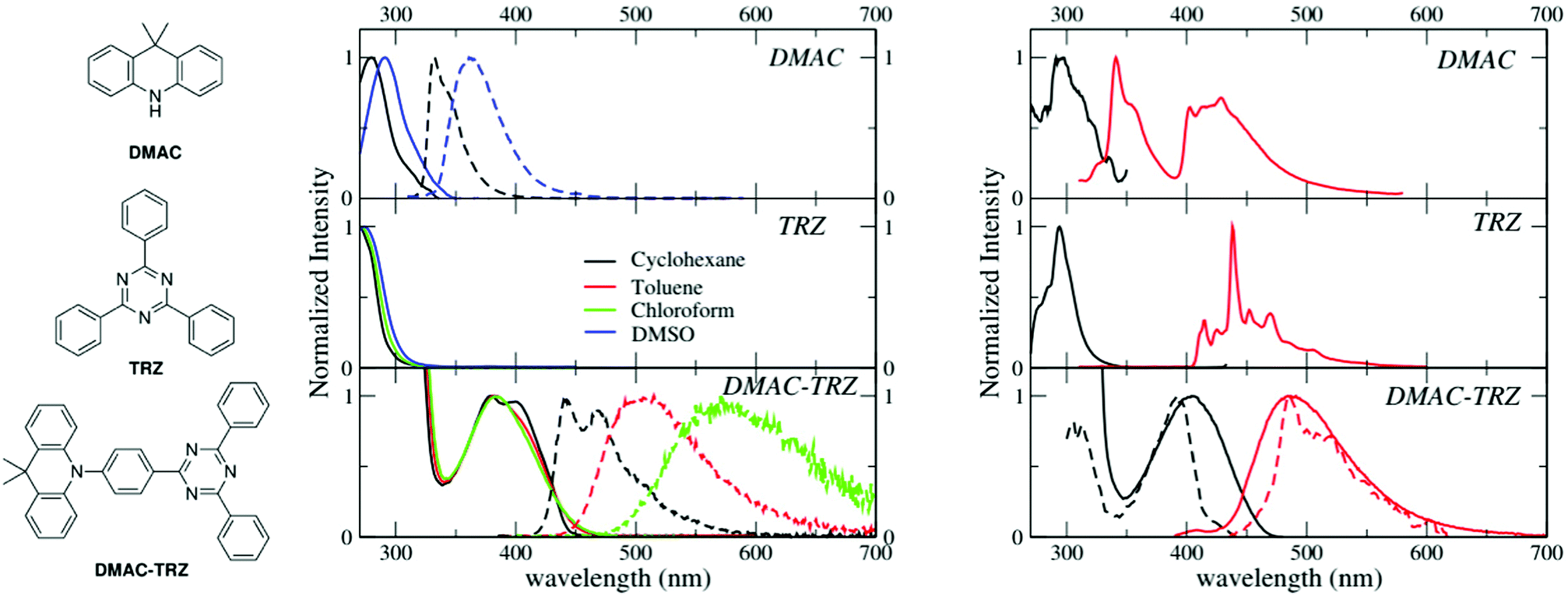 | ||
| Fig. 1 Left: Molecular structures of 9,9-dimethyl-9,10-dihydroacridine (DMAC), 2,4,6-triphenyl-1,3,5-triazine (TRZ) and DMAC-TRZ. Central panels: absorption (continuous lines) and emission spectra (dashed lines) of DMAC, TRZ and DMAC-TRZ in solvents of different polarity. Toluene, with a cut-off wavelength of 285 nm, is not suitable for DMAC and TRZ. Moreover, DMAC is not stable in chloroform, while the emission of DMAC-TRZ in DMSO is very weak. Right panels: Excitation (black) and emission (red) spectra of DMAC-TRZ in 2MeTHF at 77 K. Dashed lines in the bottom panel report gated measurements, collected with a gate delay of 1 s and a gate width of 7 s. | ||
2 Optical spectroscopy
Room temperature absorption and fluorescence spectra of DMAC-TRZ, and of the two subunits, DMAC and TRZ (Fig. 1), dissolved in solvents of different polarity (cyclohexane, toluene, chloroform and DMSO) are shown in the central panels of Fig. 1 and relevant data are summarized in Table 1. TRZ is not emissive at room temperature. Both DMAC and TRZ are transparent at λ > 350 nm, so that the weak DMAC-TRZ absorption band (molar extinction coefficient ∼2000 L mol−1 cm−1, Table S1, ESI†) observed at 380 nm is safely assigned to a CT band. Its marginal solvatochromism points to a very small permanent dipole moment for DMAC-TRZ,35 in line with a largely neutral ground state (i.e. a ground state where the contribution from the charge-separated zwitterionic DMAC+-TRZ− structure is negligible). On the opposite, DMAC-TRZ emission shows a large red-shift upon increasing the solvent polarity: the emission is therefore ascribed to a CT state, a state with a largely zwitterionic character and hence a large permanent dipole moment. The emission is safely ascribed to fluorescence, in view of its lifetime ∼10 ns (Table 1 and Fig. S2, ESI†). Indeed an emission component with longer lifetime is observed, with a sizable weight in chloroform, suggesting a possible delayed fluorescence contribution, as also supported by time resolved emission spectra (Fig. S3, ESI†) whose shape and position are time-independent.| Compound | Solvent | λ abs [nm] | λ em [nm] | Quantum yield | Lifetime [ns] |
|---|---|---|---|---|---|
| a Maximum absorption wavelength. b Maximum emission wavelength. | |||||
| DMAC | Cyclohexane | 280 | 332 | — | 2.1 (10.1%) |
| 3.9 (89.9%) | |||||
| DMSO | 291 | 361 | — | 3.6 (4.6%) | |
| 7.8 (95.4%) | |||||
| TRZ | Cyclohexane | 269 | — | — | — |
| Chloroform | 271 | — | — | — | |
| DMSO | 274 | — | — | — | |
| DMAC-TRZ | Cyclohexane | 380 | 442 | 0.22 | 9.8 (99.6%) |
| 84.5 (0.4%) | |||||
| Toluene | 382 | 510 | 0.18 | 12.7 (97.5%) | |
| 62.1 (2.5%) | |||||
| Chloroform | 382 | 571 | 0.23 | 14.4 (75%) | |
| 120.1 (25%) | |||||
The different emission bandshapes observed in polar and non-polar solvents are sometimes ascribed to an emissive state whose nature changes from LE to CT. This is easily ruled out by fluorescence excitation spectra (Fig. S4, ESI†): it is clear that, in all solvents, emission comes from the same CT state responsible for absorption. Indeed, the broadening of the emission band with increasing solvent polarity is due to the inhomogeneous broadening related to polar solvation.36–38
To address long-lived emission, including delayed fluorescence and phosphorescence, spectra were collected in a glassy 2MeTHF matrix at 77 K, as shown in Fig. 1 (right panels). DMAC shows two separate emission bands: the short wavelength band (lifetime: 5.2 ns (38%)) and 15.4 ns (62%) is due to fluorescence, while the long-wavelength band (lifetime 4 s) is ascribed to phosphorescence. A single long-lived emission (lifetime 1 s) is observed for TRZ, in the blue-green spectral region, again ascribed to phosphorescence. The emission observed for DMAC-TRZ at 485 nm, in a spectral region where neither DMAC nor TRZ emit, is clearly CT in nature. The emission decay (Fig. S5, ESI†) shows a short (of the order of ns) and a long (of the order of s) lifetime component in the same spectral region. Time resolved emission spectra are reported in Fig. S6 (ESI†). After a marginal red shift in the first few tenths of ns, the emission profile is constant in time over several order of magnitudes, as expected for TADF. Then, at ∼0.1 s the emission bandshape narrows appreciably. Dashed lines in the bottom right panel of Fig. 1 show emission and excitation spectra obtained collecting photons reaching the detector 1 s after the excitation (gated measurements, collected with a gate delay of 1 s and a gate width of 7 s). These long-delayed emission spectra are again superimposed to steady-state emission, even if with narrower bandshape, suggesting either a delayed fluorescence (even if with an unusually long lifetime) or a phosphorescence occurring in the same spectral region as fluorescence. Irrespective of the nature of this long-lived emission, the relevant excitation spectrum peaks in the same spectral region as the steady state excitation spectrum of DMAC-TRZ, i.e. in a region where neither DMAC nor TRZ show any absorption feature, demonstrating a dominant CT nature for the long-lived emission.
To gain more information on the nature of the long-lived states, Fig. 2 shows time resolved fluorescence anisotropy spectra collected up to 2 s. Anisotropy remains constant at ∼0.25 up to at least 10 ms, and then decreases. The constant and large value of the emission anisotropy over 6 orders of magnitude in time (from ns to ms), and the invariance of emission spectra in the same temporal windows (Fig. S6, ESI†) unambiguously point to the observation of delayed fluorescence up to ∼10 ms. At longer times, the anisotropy decreases (Fig. 2 bottom panel), and the shape of emission spectra (but not their position) changes (Fig. S6, ESI,† and Fig. 1), offering a clear evidence of the involvement of a different emissive state, corresponding to a very long-lived triplet state. As discussed above, this triplet state has a CT nature, since the corresponding excitation spectrum (black dashed line in Fig. 1) is distinctively red-shifted with respect to the absorption spectra of either DMAC or TRZ subunits. The marked decrease of the anisotropy for the phosphorescence signal can be understood in terms of a small mixing of the CT triplet state with an LE triplet. Transition dipole moments associated with (weak) CT transitions are orders of magnitude smaller than those relevant to LE states: even a weak LE contribution to the phosphorescent state would dominate the observed transition dipole moment, being therefore responsible for its rotation with respect to the CT direction.
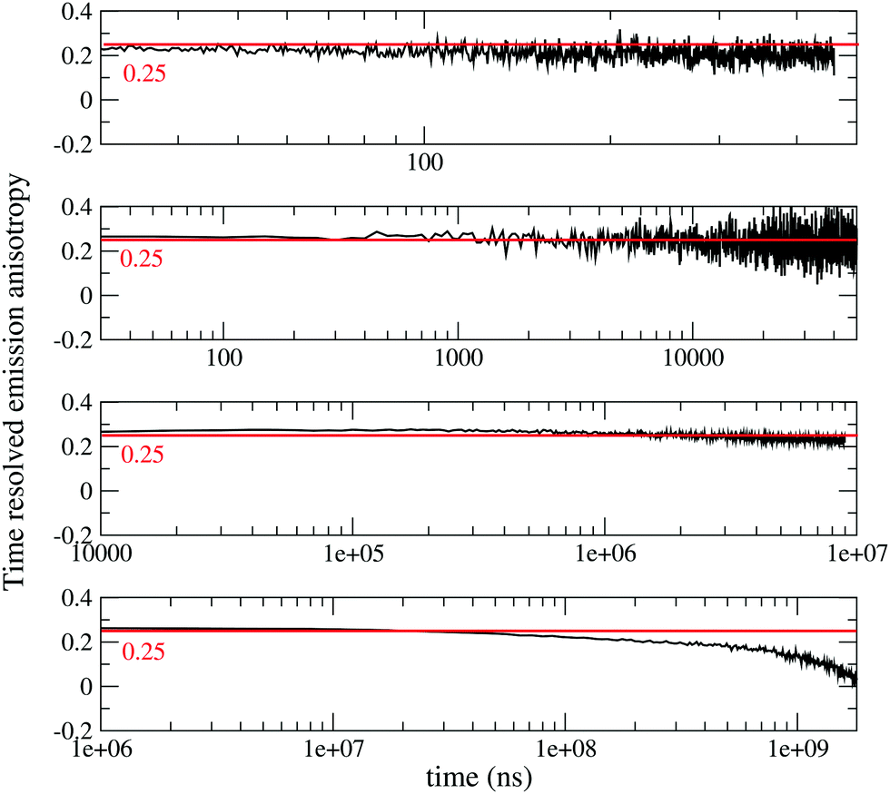 | ||
| Fig. 2 Time-resolved anisotropy of DMAC-TRZ collected in 2MeTHF at 77 K in different time ranges (excitation wavelegth 405 nm, emission wavelength 485 nm). | ||
3 Computational analysis
The ground state geometry of DMAC-TRZ is optimized in DFT (B3LYP/6-31G(d)) in Gaussian 16 B.10.39 The equilibrium dihedral angle, θ in Fig. 3a, amounts to 90°, suggesting a negligible delocalization of electrons between the donor (DMAC) and acceptor (TRZ) units. To address excited states in such a large molecule, TD-DFT is the method of choice and, being interested in both singlet and triplet states, we adopt the Tamm–Dancoff approximation.40 The most delicate issue is the choice of the functional. Recent studies propose the use of range-separated exchange functionals to solve the problem for CT states, optimizing ω, the range-separation parameter, for each molecule of interest.41–43 Fairly reliable results for TADF-dyes are obtained in the optimal long-range corrected PBE (LC-ω*PBE, see ESI,† for additional details).43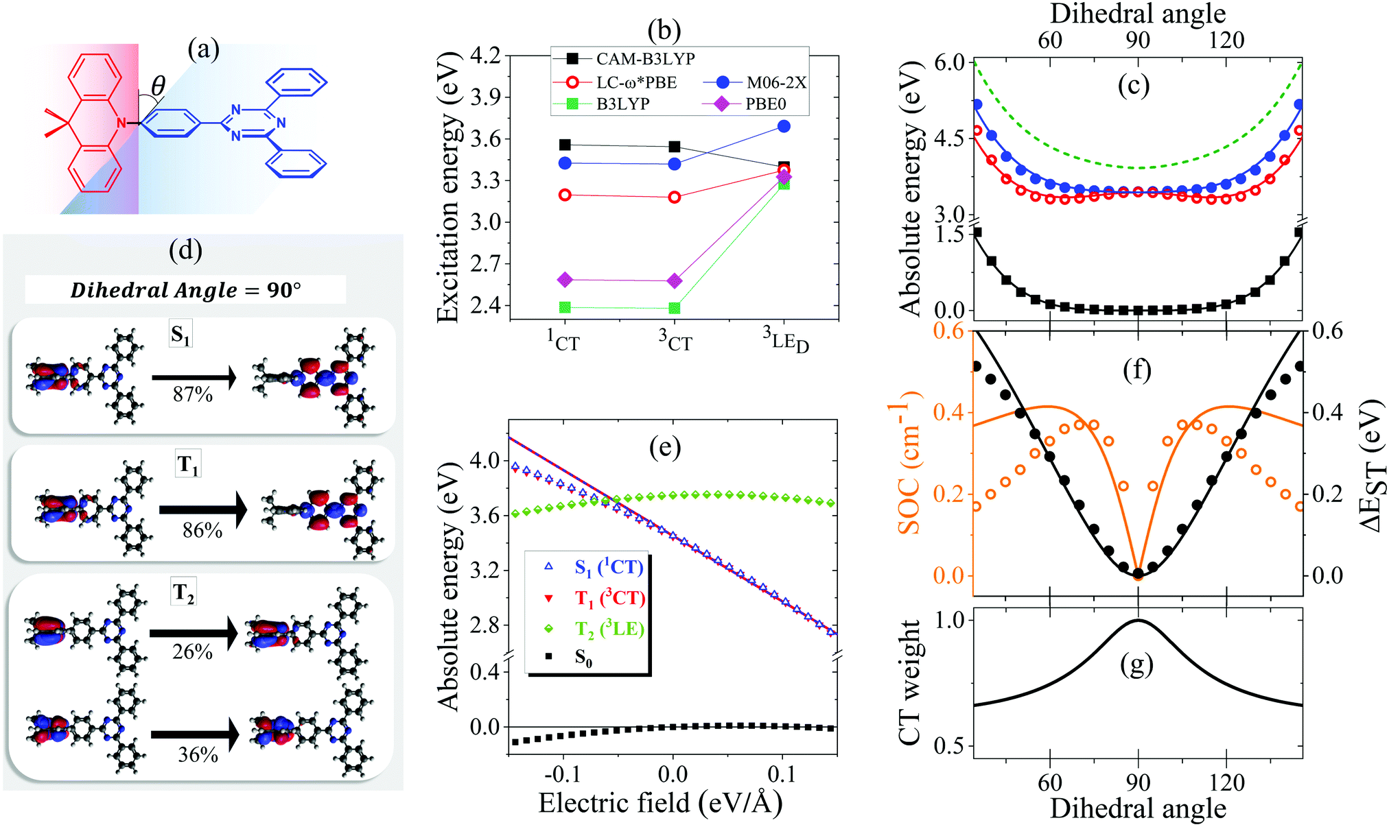 | ||
| Fig. 3 (a) A sketch of DMAC-TRZ, showing the dihedral angle, (b) excitation energies for the three lowest excited states calculated at the equilibrium geometry with different functionals. (c) The energy of the ground (black), lowest excited singlet (blue) and triplet (red) states calculated as a function of θ in TD-DTF (symbols) and ESM (lines). The green dashed line shows the effective LE triplet introduced in the ESM. (d) Natural transition orbitals of the lowest singlet excited state and of the two-lowest triplet states. (e) Energies of the four lowest states vs. the applied field (results for transition energies are shown in Fig. S10, ESI†) (f) The singlet–triplet gap (black) and the spin–orbit coupling (orange) between the lowest singlet and triplet states vs. θ. Symbols and lines refer to TD-DFT and ESM results, respectively. (g) The weight of the CT state in the lowest triplet as estimated in ESM. | ||
Excitation energies of DMAC-TRZ, reported in Fig. 3b for the lowest singlet and triplet states, are obtained for the optimized ω = 0.195 value (see ESI†) and are compared with results obtained with B3LYP,44 CAM-B3LYP45 and M06-2X functionals.46 While all functionals find almost degenerate singlet and triplet states with a dominant CT character, the relative energies of CT and LE states change wildly, with B3LYP and PBE0 largely underestimating the energy of CT states and CAM-B3LYP overestimating it. M06-2X slightly overestimates all transition energies, but gives a very similar trend as LC-ω*PBE functional for the excitation energies of singlet and triplet states. Results in Fig. 3b refer to the equilibrium geometry, θ = 90°, but similar results were obtained for few selected values of the dihedral angle (Fig. S7, ESI†). On this basis, M06-2X is adopted as functional of choice.
Fig. 3 summarizes main TD-DFT results. At the equilibrium geometry, the planes of DMAC and TRZ moieties are mutually orthogonal (θ = 90°) and the lowest lying singlet and triplet states (S1 and T1, respectively) are almost degenerate. The next excited state T2, at 3.75 eV (not shown in the figure), is again a triplet. Based on relevant natural transition orbitals (Fig. 3d) we describe the two lowest and almost degenerate singlet and triplet states as CT states (1CT and 3CT, respectively), while the next excited state is a triplet state localized on donor unit (3LED). To further confirm the nature of the states, Fig. 3e shows the evolution of the energies of the lowest states vs. an electric field applied along the D–A axis. The energy of the ground (S0) and of the T2 state marginally depends on the applied field, suggesting that the two states have a very small permanent dipole moment, confirming the local nature of T2. On the opposite, the large and almost linear dependence of the energy of S1 and T1 states on the applied field, points to a large and almost constant dipole moment for both states, confirming their CT nature.
The pure CT nature of the lowest singlet and triplet states accounts for a vanishing singlet–triplet gap, ΔEST = 0, but, according to the El-Sayed rule,11 it also implies a negligible spin–orbit coupling, hindering RISC and hence TADF. To better understand the physics of TADF in DMAC-TRZ, we therefore calculate the energies of the relevant states upon varying the dihedral angle, while keeping the geometry of the two fragments fixed. Results in Fig. 3c are interesting in several respect. First of all, the potential associated to the ground state and to the first singlet state is fairly flat, suggesting considerable thermal configurational disorder. Moreover, a double-minimum structure is observed for the lowest triplet state: the equilibrium conformation for the relaxed triplet has a twist angle θ ∼ 60° or 120°. As discussed in the next section, this variation of conformation in the triplet state can only be rationalized accounting for the coupling with some higher energy (local) excited triplet state. Fig. 3f finally summarizes results of interest for TADF: the θ-dependence of the singlet–triplet gap and of the corresponding spin–orbit coupling. As expected, the singlet–triplet gap increases as the mutual orientation of the D and A planes deviates from orthogonality, at the same time the spin–orbit coupling first increases, to decrease again for 75° < θ< 105°.
The comparison with experiment requires a careful analysis of solvation effects, typically dealt with approximating the solvent as a continuum dielectric medium.47 However, as discussed in a recent paper,48 current implementations of continuum solvation models in quantum chemical packages do not properly account for the role of the solvent electronic polarizability, leading to results that, as shown in Fig. S9 (ESI†) for the available implementations of the polarizable continuum model in Gaussian 16,39 wildly depend on the specific approximation scheme adopted, already in the comparatively simple case of a non-polar solvent. In the following section we will therefore develop a minimal model for DMAC-TRZ that will allow us to discuss solvation and matrix effects in a simple and reliable approach.
4 Understanding TADF: conformational disorder and matrix effects
4.1 Setting up the model
Having collected a large amount of experimental data and of computational results, we are now in the position to set up a model for DMAC-TRZ. In the spirit of essential state models (ESM)36,37,49,50 we select the minimal set of electronic diabatic basis states to describe the ground and the low-energy excited states. As for singlet states, the two-state model, proposed and extensively validated for D–A dyes,36,37,51 also applies to DMAC-TRZ. The electronic basis states are selected as the neutral DA state, N, and the zwitterionic D+A− state, Z. The two states are separated by an energy difference 2z and are mixed by a matrix element −τ, as sketched in Fig. 4. As discussed above, the orthogonal configuration of the D and A planes, suggests a vanishing τ at the equilibrium so that the ground state S0 and the first excited state S1 basically coincide with N and Z, respectively.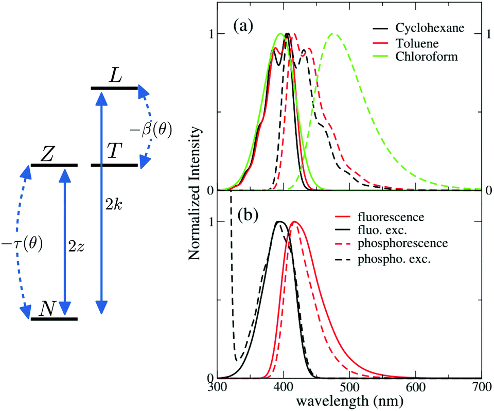 | ||
| Fig. 4 Left: Schematic representation of the four electronic basis states entering the ESM model for DMAC-TRZ. Right panels: spectra calculated in the complete ESM also accounting for vibrational and conformational degrees of freedom and environmental effects. (a) Absorption and fluorescence spectra (continuous and dashed lines, respectively) of DMAC-TRZ in solvents of different polarity at 298 K. (b) Calculated spectra in frozen 2MeTHF. Continuous lines: calculated fluorescence and fluorescence excitation spectra. Dashed lines: phosphorescence and phosphorescence excitation spectra. Excitation spectra are computed setting the excitation wavelength at 412 nm. The temperature was set to 77 K in the calculation of the Boltzmann distribution along the conformational coordinate, while it was set to 91 K (matching 2MeTHF glass transition temperature) for the Boltzmann distribution along the solvation coordinate. | ||
To account for the lowest triplet state, the basis must be extended to account for the zwitterionic triplet state T. The energy of the singlet and triplet zwitterionic basis states, Z and T, is the same, and, according to the El-Sayed rule, the spin–orbit coupling between the two states vanishes. A small but finite spin–orbit coupling Vsoc instead mixes T with N. The relevant 3 × 3 Hamiltonian matrix can be found in the ESI.†
We are interested to reproduce the θ dependence of the calculated energies of the excited singlet and triplet states in Fig. 3c. To this aim, the spin orbit coupling Vsoc can be treated as a minor perturbation, so that, at the lowest order, only two electronic parameters enter the three state model: 2z whose marginal θ-dependence is neglected, and τ whose dependence on θ is definitely relevant. Information on the τ(θ) dependence can be extracted mapping TD-DFT results on ESM. Specifically, in ESM the product between the transition frequency and the transition dipole moment is proportional to τ.52 Relevant TD-DFT results in Fig. S12 (ESI†) are fully consistent with τ(θ) = τ0|cos(θ)|. Of course we must also introduce a restoring potential that we set equal for all states, in the hypothesis that state-specific features can be reproduced by the ESM, provided the relevant physics is properly accounted for. The restoring potential is set via an expansion to the fourth order around the equilibrium V(δ) = a2δ2 + a4δ4, where δ = θ–90°. Irrespective of model parameters, in the three-state model the triplet state only marginally mixes with the singlet state and therefore the relevant potential energy curve cannot develop the double minimum calculated in TD-DFT (Fig. S11, ESI†).
A TD-DFT analysis of the nature of the lowest triplet state shows that it is a pure CT state at θ = 90°, but it acquires some local nature when the system deviates from orthogonality. Unfortunately, several local triplet states enter into play and including all of them would lead to an impractical ESM, with too many parameters. On the other hand, we are not interested to model in detail higher excited triplets, rather we just want to capture the effect of their mixing with T1. We therefore set up a four-state model that, besides the three states, |N〉, |Z〉 and |T〉, described above, also includes an effective local triplet state |L〉 whose energy, 2k is a free fitting parameter. As for the mixing matrix element with T we assume the same angular dependence as for τ, setting β(θ) = β0|cos![[thin space (1/6-em)]](https://www.rsc.org/images/entities/char_2009.gif) θ|. The relevant Hamiltonian, on the |N〉, |Z〉, |T〉 and |L〉 basis, reads:
θ|. The relevant Hamiltonian, on the |N〉, |Z〉, |T〉 and |L〉 basis, reads:
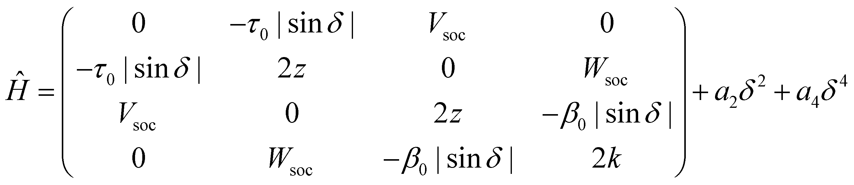 | (1) |
The spin–orbit coupling elements, Vsoc and Wsoc, are very small and do not appreciably affect the calculated potential energy curves. To reproduce TD-DFT results model parameters are set to the values in Table 2. The agreement is very satisfactory (Fig. 3c), suggesting that the proposed ESM properly captures the low-energy physics of the system. Quite interestingly, the lowest triplet state, the one relevant to TADF, has a pure CT character at 90°, but it acquires a partial local character at the equilibrium geometry (Fig. 3g), as also confirmed by the analysis of the evolution with the dihedral angle of the natural transition orbitals calculated for T1 state in Fig. S8 (ESI†).
| z (eV) | 1.72 |
| τ 0 (eV) | 0.75 |
| k (eV) | 1.96 |
| β 0 (eV) | 0.85 |
| a 2 (eV) | 6.00 × 10⁻⁵ |
| a 4 (eV) | 1.43 × 10⁻⁷ |
The specific and somewhat arbitrary choice made for the effective local triplet state, does not alter the main picture. In Fig. S13 of the ESI,† we compare results obtained with models parameters in Table 2, with those obtained for different choices for the effective triplet state, and specifically we show results for a system where the state has a larger energy and a larger coupling strength and one where two coupled local triplet states are considered. Results are marginally affected by the choice: the θ-dependence of relevant electronic states and the of the SOC magnitude are in fact governed by the nature of the lowest triplet state, and more precisely by the weight in this state of the CT triplets, while the precise properties of the effective triplet state(s) play a marginal role, as also demonstrated by calculated spectra (see the Discussion in Section 4.2 and Fig. S15 in the ESI†).
Since at the equilibrium geometry the ground state S0 and T1 practically coincide with |N〉 and |T〉, respectively, we set Vsoc = 3.84 × 10⁻⁴ eV equal to the TD-DFT value for the spin–orbit coupling between S0 and T1 states. Finally, the value of Wsoc = 1.74 × 10⁻⁴ eV is adjusted in order to match the θ-dependence of the S1–T1 SOC (Fig. 3f).
4.2 Validating the model against steady-state spectra
Having built and parametrized against TD-DFT the electronic model for DMAC-TRZ, we now validate it against experimental spectra in Section 2. Towards this aim, the model must be extended to account for electron–vibration coupling and for solvation effects, as to address the observed vibronic structure and solvatochromism.Typically, ESMs for D–A dyes describe electron–vibration coupling in terms of a single effective coordinate Q that accounts for the different geometry of the neutral and charge-separated diabatic states.36,37,51 For DMAC-TRZ, the frequency of the effective coordinate is easily estimated as ωv ∼ 0.18 eV from the partially resolved vibronic structure of optical spectra in non-polar solvents. The strength of the coupling is measured by the vibrational relaxation energy, εv, the energy gained by the charge separated (either Z or T) states upon relaxation. From DFT energies of the isolated D and D+ and A and A− species we extract εv ∼ 0.17 eV (see ESI†).
The simplest solvation model describes the solvent as a continuum elastic medium that responds to the presence of a solute molecule generating at the solute location an electric field, called the reaction field, proportional to the solute dipole moment. As extensively discussed in ref. 48, two components of the reaction field must be considered, a fast component associated to the electronic polarizability of the solvent and a slow component, of interest for polar solvents, associated with the orientational motion of the solvent molecules. The fast solvation component can be treated in the antiadiabatic approximation leading to a renormalization of the z parameter.53 In the hypothesis that the solute occupies a spherical cavity of radius a inside the solvent, the renormalized z reads:
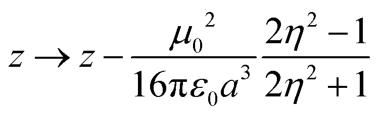 | (2) |
The slow component of the reaction field For enters the model as a slow coordinate and can be treated in the adiabatic approximation. The total Hamiltonian then reads
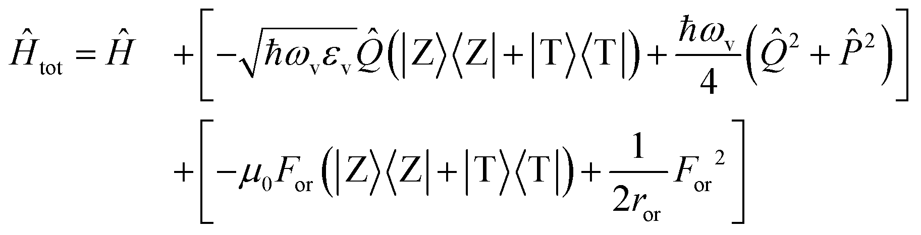 | (3) |
![[P with combining circumflex]](https://www.rsc.org/images/entities/i_char_0050_0302.gif) being the momentum operator associated to the coordinate
being the momentum operator associated to the coordinate ![[Q with combining circumflex]](https://www.rsc.org/images/entities/i_char_0051_0302.gif) . The second square bracket collects polar solvation terms, with ror defined as
. The second square bracket collects polar solvation terms, with ror defined as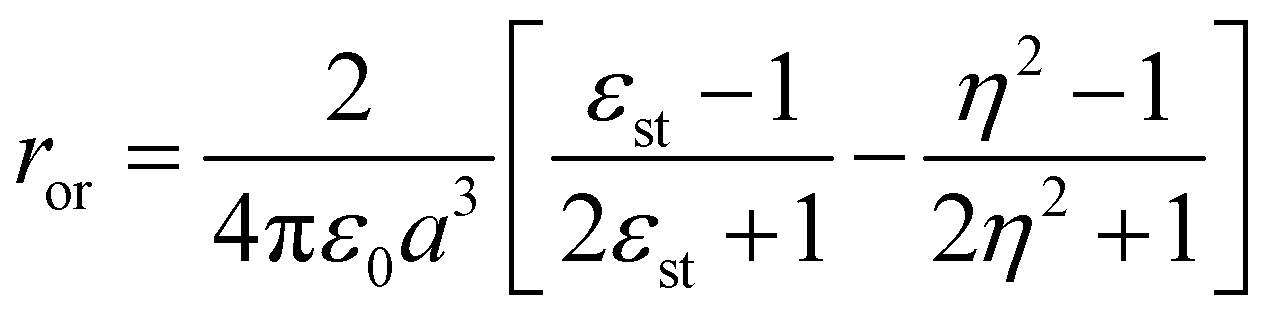 | (4) |
We solve the model Hamiltonian in eqn (3), writing the corresponding Hamiltonian matrix, for fixed For and δ values, on the basis obtained as the direct product of the 4-dimensional electronic basis states times the first M states of the harmonic oscillator associated to the vibrational coordinate . M is large enough (typically in this work M = 10) to ensure convergence. The Hamiltonian matrix is then diagonalized numerically to get vibronic eigenstates. Absorption and fluorescence spectra are computed assigning to each transition a Gaussian bandshape with a half-width at half-maximum of Γ = 0.08 eV. Spectra calculated for different For and δ values are then summed over accounting for their Boltzmann weight with reference to the energy of the ground state for absorption spectra, and of the lowest singlet and triplet states for fluorescence and phosphorescence spectra, respectively.49
Calculated absorption and fluorescence spectra in solvents of different polarity are shown in Fig. 4a. Absorption spectra agree well with experimental results in Fig. 1 (see also Fig. S14, ESI† for an easy comparison), showing negligible solvatochromism. Emission spectra qualitatively agree with experiment, reproducing the observed solvatochromism and the bandshape evolution with solvent polarity. The Stokes shift is overall underestimated with respect to experiment, possibly suggesting the presence of other sources of conformational disorder. We unerline that quantitative agreement (Fig. S14, ESI†) can be obtained if εor is treated as an adjustable parameter, accounting for all relaxation phenomena and relaxing the crude approximation of a spherical solvent cavity.
4.3 Matrix effect
The model developed and validated for DMAC-TRZ in liquid solutions also applies to DMAC-TRZ in solid matrices, at least as long as the concentration is low enough to neglect intermolecular interactions. As a rule of thumb, concentrations ∼1% result, for typical matrix density ∼1 g cm−3, in an average distance between dyes of the order of few nm. Up to these concentrations electrostatic intermolecular interactions can be safely neglected. In diluted solid matrices, the solvent molecules surrounding the solute do not readjust following the solute excitation, while the conformational flexibility of DMAC-TRZ is maintained. In this hypothesis, we calculate fluorescence and fluorescence excitation spectra of DMAC-TRZ in frozen 2MeTHF at 77 K as shown in Fig. 4b. As discussed in the previous section for absorption and fluorescence in liquid solvents, also in this case the calculated Stokes shifts are somewhat underestimated, but a good agreement with experimental results in Fig. 2 is obtained in terms of bandshape and band positions.More delicate and interesting is the calculation of phosphorescence and phosphorescence excitation spectra. Phosphorescence is a forbidden process that occurs because spin–orbit coupling generates a very small mixing of singlet and triplet states. As a result, the triplet state borrows a tiny transition dipole moment from the singlet states. The lowest triplet state in DMAC-TRZ is described as the CT triplet plus a minor but non negligible contribution from a local triplet state. Phosphorescence intensity then has a contribution from the (tiny) transition dipole moments associated with CT and LE triplets. Since the transition dipole moments associated with CT states are orders of magnitude lower than the transition dipole moments associated with LE states, we assume that the contribution to phosphorescence from the LE state dominates over the contribution from the CT state. This hypothesis is also supported by the decrease of the emission anisotropy at very long delay times (Fig. 2). Accordingly, phosphorescence and phosphorescence excitation spectra in Fig. 4b are calculated only accounting for the LE contribution to the transition dipole moment (spectra calculated accounting only for the CT contribution in Fig. S16 (ESI†) are in any case very similar). Calculated spectra in Fig. 4b, referring to glassy 2MeTHF matrix at 77 K, compare very well with experimental results of Fig. 1. Of course we only address phosphorescence bandshapes, the intensity of this process is very low and in any case it is not accessible experimentally.
Low-T spectra are of special interest to collect reasonably intense phosphorescence spectra, but the model of course applies to the calculation of spectra at any temperature. Indeed temperature enters in the definition of the Boltzmann distribution relevant to the ground state (for absorption and excitation spectra) or to the relevant excited state for fluorescence and phosphorescence spectra. Increasing the temperature then leads to a broadening of the spectra, as shown in Fig. S17 (ESI†) that shows room temperature spectra calculated for DMAC-TRZ dissolved in a matrix with the same dielectric properties adopted for glassy 2-MeTHF.
The spectroscopic effects of polar solvation are well documented experimentally,35 well understood in terms of simple solvation models35,37,54,55 and are reliably addressed in current implementations of continuum solvation models in quantum chemical calculations.47,56,57 The role of the electronic polarizability of the solvent (including rigid matrices) is more delicate. The marginal variability of the refractive index in common organic matrices makes an experimental analysis very difficult, while available implementations of continuum solvation models in quantum chemical approaches do not treat the corresponding solvation contribution properly.48 However a sound understanding of the effects of the environmental polarizability on TADF-dyes is important in order to concurrently optimize the dye in its matrix, in the so called smart matrix approach. Specifically, the important information extracted from quantum chemical calculations for a dye in the gas phase cannot be transferred directly to a solvated dye, not even to a dye in a comparatively simple environment like a non-polar solvent. To illustrate this point we now discuss how the properties of DMAC-TRZ vary from gas-phase to a non-polar matrix with refractive index η = 2, taken as an upper limit, typical refractive index of common matrices being in the 1.5–1.7 range.
Specifically, Fig. 5 shows the evolution with the dihedral angle, θ, of the energy of the first excited triplet and singlet and of the corresponding spin–orbit coupling. The first effect of the solvent polarizability is a considerable red-shift of CT states, that shows up with a marked red-shift of absorption and emission bands (see Fig. S18, ESI†). However, the most important effect of the environmental polarizability is expected on the properties that govern TADF. Indeed, since environmental effects are minor for LE states, the energy gap between CT and LE triplet increases, so that overall the spin–orbit coupling decreases, an effect that is clearly unfavorable for TADF applications. There is however another effect of the environmental polarizability: the potential energy curve associated to the lowest triplet is flatter in the matrix than in gas phase. Accordingly, a larger region is found where the singlet–triplet gap is thermally accessible (the shaded areas in the figure mark the inaccessible regions, those where the gap is larger than thermal energy at ambient conditions). Even more important, because of the shallower potential energy curve for the lowest triplet state, the distribution of θ equilibrated to the lowest triplet state is much broader in the matrix than in the gas phase. This is relevant, since TADF occurs from the equilibrated lowest triplet state and in the gas-phase the population of conformations with thermally accessible RISC is marginal, while it becomes sizable in the matrix. This of course considerably favors TADF, possibly outweighting the decrease of the spin–orbit coupling among states responsible for RISC.
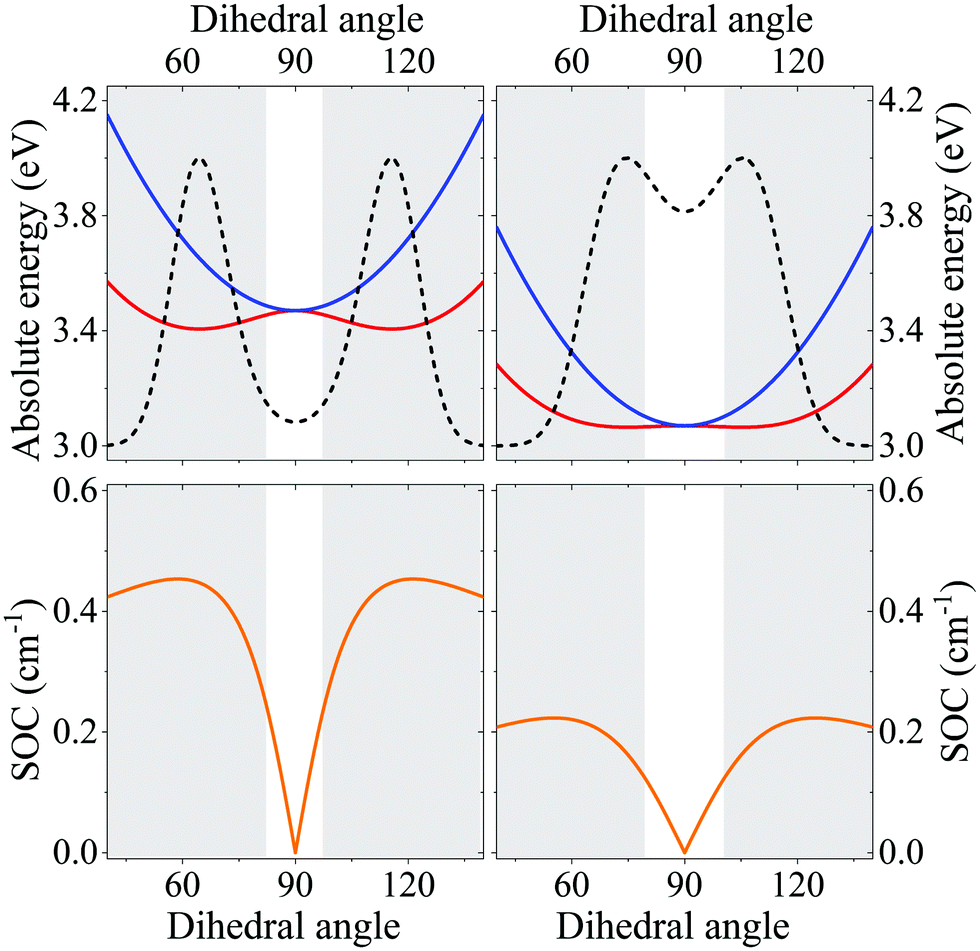 | ||
| Fig. 5 Comparison of ESM model results for DMAC-TRZ in the gas phase (left) and in a non-polar matrix with refractive index η = 2 (right). Top panels show the θ-dependence of the energies of the lowest excited singlet (blue) and triplet (red) states. The dotted line show the Boltzmann distribution calculated for the lowest triplet state. Bottom panels show the θ-dependence of the spin–orbit coupling between the lowest excited singlet and triplet states. The shaded areas mark the regions where the singlet triplet gap is larger than thermal energy at ambient conditions. | ||
5 Conclusions
We presented thorough experimental and theoretical analysis of DMAC-TRZ, a prototypical dye for TADF applications. Experimental results unambiguously demonstrate that a state with predominant CT nature is responsible for fluorescence and delayed fluorescence. Phosphorescence occurs in the same spectral region as fluorescence, from a triplet state with dominant CT character. Extensive gas-phase TD-DFT calculations, run in the presence of an applied electric field and for different conformations, confirm the experimental analysis and are exploited to build a reliable essential-state model for DMAC-TRZ. The model accounts for few electronic states, as needed to describe the low-energy properties of the dye, for the coupling to a molecular vibration, responsible for the vibronic structure of the absorption and fluorescence bands, and for the conformational degrees of freedom associated with the torsional angle that modulates spin–orbit coupling. Environmental effects are properly addressed to simulate spectral properties in liquid solution and solid matrices, accounting for the different role of polar solvation and of the electronic polarizability of the environment. The resulting picture, extensively validated against experiment, offers a sturdy and flexible toy model to investigate TADF.The approach proposed here for a specific dye is general and can be applied to set up reliable few-state models for other dyes, including multipolar dyes, with multiple D and A groups. The enormous variability of the properties of these dyes, depending on the number and strength of the D and A groups, on bridging units and geometry,6 calls for the definition of practical models to define reliable structure–properties relationships for the large and technologically relevant family of TADF dyes. The power of few-state models is in the possibility to account for a large number of interactions that range from vibrational coupling, to be treated in a truly non-adiabatic approach, conformational motion, treated adiabatically, and the interaction with the local environment, accounting for both the polarizability and the polarity of the environment. The model also sets the basis to build an open-quantum model58,59 for TADF dyes able to address ISC and RISC processes, together with other competitive relaxation process without introducing additional approximations. The evolution of the population of excited states can be followed over several orders of magnitude in time, to trace the subtle competition between fluorescence, phosphorescence, non-radiative relaxation, ISC, RISC that govern the delicate TADF phenomenon, shedding a clear light on and their interdependence with vibrational and conformational motions and on environmental effects.
Conflicts of interest
There are no conflicts to declare.Acknowledgements
This project received funding from the European Union Horizon 2020 research and innovation programme under Grant Agreement No. 812872 (TADFlife), and benefited from the equipment and support of the COMP-HUB Initiative, funded by the “Departments of Excellence” program of the Italian Ministry for Education, University and Research (MIUR, 2018–2022). We acknowledge the support from the HPC (High Performance Computing) facility of the University of Parma, Italy.References
- C. A. Parker and C. G. Hatchard, Trans. Faraday Soc., 1961, 57, 1894–1904 RSC.
- A. Endo, K. Sato, K. Yoshimura, T. Kai, A. Kawada, H. Miyazaki and C. Adachi, Appl. Phys. Lett., 2011, 98, 083302 CrossRef.
- H. Uoyama, K. Goushi, K. Shizu, H. Nomura and C. Adachi, Nature, 2012, 492, 234–238 CrossRef CAS.
- C. Adachi, Jpn. J. Appl. Phys., 2014, 53, 060101 CrossRef.
- M. Y. Wong and E. Zysman-Colman, Adv. Mater., 2017, 29, 1605444 CrossRef.
- F.-M. Xie, J.-X. Zhou, Y.-Q. Li and J.-X. Tang, J. Mater. Chem. C, 2020, 8, 9476–9494 RSC.
- D. Barman, R. Gogoi, K. Narang and P. K. Iyer, Front. Chem., 2020, 8, 483 CrossRef CAS.
- J. Lee, K. Shizu, H. Tanaka, H. Nomura, T. Yasuda and C. Adachi, J. Mater. Chem. C, 2013, 1, 4599 RSC.
- F. B. Dias, K. N. Bourdakos, V. Jankus, K. C. Moss, K. T. Kamtekar, V. Bhalla, J. Santos, M. R. Bryce and A. P. Monkman, Adv. Mater., 2013, 25, 3707–3714 CrossRef CAS.
- Z. Yang, Z. Mao, Z. Xie, Y. Zhang, S. Liu, J. Zhao, J. Xu, Z. Chi and M. P. Aldred, Chem. Soc. Rev., 2017, 46, 915–1016 RSC.
- M. A. El-Sayed, J. Chem. Phys., 1963, 38, 2834–2838 CrossRef CAS.
- R. S. Mulliken, J. Am. Chem. Soc., 1952, 74, 811–824 CrossRef CAS.
- T. Jiang, Y. Liu, Z. Ren and S. Yan, Polym. Chem., 2020, 11, 1555–1571 RSC.
- M. K. Etherington, F. Franchello, J. Gibson, T. Northey, J. Santos, J. S. Ward, H. F. Higginbotham, P. Data, A. Kurowska, P. L. Dos Santos, D. R. Graves, A. S. Batsanov, F. B. Dias, M. R. Bryce, T. J. Penfold and A. P. Monkman, Nat. Commun., 2017, 8, 14987 CrossRef CAS.
- T. J. Penfold, F. B. Dias and A. P. Monkman, Chem. Commun., 2018, 54, 3926–3935 RSC.
- C. S. Oh, D. de Sa Pereira, S. H. Han, H.-J. Park, H. F. Higginbotham, A. P. Monkman and J. Y. Lee, ACS Appl. Mater. Interfaces, 2018, 10, 35420–35429 CrossRef CAS.
- F. B. Dias, J. Santos, D. R. Graves, P. Data, R. S. Nobuyasu, M. A. Fox, A. S. Batsanov, T. Palmeira, M. N. Berberan-Santos, M. R. Bryce and A. P. Monkman, Adv. Sci., 2016, 3, 1600080 CrossRef.
- P. K. Samanta, D. Kim, V. Coropceanu and J.-L. Brédas, J. Am. Chem. Soc., 2017, 139, 4042–4051 CrossRef CAS.
- X.-K. Chen, D. Kim and J.-L. Brédas, Acc. Chem. Res., 2018, 51, 2215–2224 CrossRef CAS.
- X.-K. Chen, S.-F. Zhang, J.-X. Fan and A.-M. Ren, J. Phys. Chem. C, 2015, 119, 9728–9733 CrossRef CAS.
- J. Gibson, A. P. Monkman and T. J. Penfold, ChemPhysChem, 2016, 17, 2956–2961 CrossRef CAS.
- M. K. Etherington, J. Gibson, H. F. Higginbotham, T. J. Penfold and A. P. Monkman, Nat. Commun., 2016, 7, 13680 CrossRef CAS.
- I. Lyskov and C. M. Marian, J. Phys. Chem. C, 2017, 121, 21145–21153 CrossRef CAS.
- T. J. Penfold, E. Gindensperger, C. Daniel and C. M. Marian, Chem. Rev., 2018, 118, 6975–7025 CrossRef CAS.
- G. Méhes, K. Goushi, W. J. Potscavage and C. Adachi, Org. Electron., 2014, 15, 2027–2037 CrossRef.
- P. L. dos Santos, J. S. Ward, M. R. Bryce and A. P. Monkman, J. Phys. Chem. Lett., 2016, 7, 3341–3346 CrossRef CAS.
- H. Sun, Z. Hu, C. Zhong, X. Chen, Z. Sun and J.-L. Brédas, J. Phys. Chem. Lett., 2017, 8, 2393–2398 CrossRef CAS.
- T. Northey, J. Stacey and T. J. Penfold, J. Phys. Chem. C, 2017, 5, 11001–11009 CAS.
- Y. Olivier, B. Yurash, L. Muccioli, G. D'Avino, O. Mikhnenko, J. C. Sancho-García, C. Adachi, T.-Q. Nguyen and D. Beljonne, Phys. Rev. Mater., 2017, 1, 075602 CrossRef.
- Y. Olivier, J.-C. Sancho-Garcia, L. Muccioli, G. DâĂŹAvino and D. Beljonne, J. Phys. Chem. Lett., 2018, 9, 6149–6163 CrossRef CAS.
- J.-M. Mewes, Phys. Chem. Chem. Phys., 2018, 20, 12454–12469 RSC.
- R. Skaisgiris, T. Serevičius, K. Kazlauskas, Y. Geng, C. Adachi and S. Juršėnas, J. Mater. Chem. C, 2019, 7, 12601–12609 RSC.
- K. Stavrou, L. G. Franca and A. P. Monkman, ACS Appl. Electron. Mater., 2020, 2, 2868–2881 CrossRef CAS.
- W.-L. Tsai, M.-H. Huang, W.-K. Lee, Y.-J. Hsu, K.-C. Pan, Y.-H. Huang, H.-C. Ting, M. Sarma, Y.-Y. Ho, H.-C. Hu, C.-C. Chen, M.-T. Lee, K.-T. Wong and C.-C. Wu, Chem. Commun., 2015, 51, 13662–13665 RSC.
- C. Reichardt, Chem. Rev., 1994, 94, 2319–2358 CrossRef CAS.
- A. Painelli and F. Terenziani, J. Phys. Chem. A, 2000, 104, 11041–11048 CrossRef CAS.
- B. Boldrini, E. Cavalli, A. Painelli and F. Terenziani, J. Phys. Chem. A, 2002, 106, 6286–6294 CrossRef CAS.
- F. Terenziani and A. Painelli, Phys. Chem. Chem. Phys., 2015, 17, 13074–13081 RSC.
- M. J. Frisch, G. W. Trucks, H. B. Schlegel, G. E. Scuseria, M. A. Robb, J. R. Cheeseman, G. Scalmani, V. Barone, G. A. Petersson, H. Nakatsuji, X. Li, M. Caricato, A. V. Marenich, J. Bloino, B. G. Janesko, R. Gomperts, B. Mennucci, H. P. Hratchian, J. V. Ortiz, A. F. Izmaylov, J. L. Sonnenberg, D. Williams-Young, F. Ding, F. Lipparini, F. Egidi, J. Goings, B. Peng, A. Petrone, T. Henderson, D. Ranasinghe, V. G. Zakrzewski, J. Gao, N. Rega, G. Zheng, W. Liang, M. Hada, M. Ehara, K. Toyota, R. Fukuda, J. Hasegawa, M. Ishida, T. Nakajima, Y. Honda, O. Kitao, H. Nakai, T. Vreven, K. Throssell, J. A. Montgomery, Jr., J. E. Peralta, F. Ogliaro, M. J. Bearpark, J. J. Heyd, E. N. Brothers, K. N. Kudin, V. N. Staroverov, T. A. Keith, R. Kobayashi, J. Normand, K. Raghavachari, A. P. Rendell, J. C. Burant, S. S. Iyengar, J. Tomasi, M. Cossi, J. M. Millam, M. Klene, C. Adamo, R. Cammi, J. W. Ochterski, R. L. Martin, K. Morokuma, O. Farkas, J. B. Foresman and D. J. Fox, Gaussian 16 Revision B.01 Search PubMed.
- S. Hirata and M. Head-Gordon, Chem. Phys. Lett., 1999, 314, 291–299 CrossRef CAS.
- T. Stein, L. Kronik and R. Baer, J. Am. Chem. Soc., 2009, 131, 2818–2820 CrossRef CAS.
- H. Sun and J. Autschbach, ChemPhysChem, 2013, 14, 2450–2461 CrossRef CAS.
- H. Sun, C. Zhong and J.-L. Brédas, J. Chem. Theory Comput., 2015, 11, 3851–3858 CrossRef CAS.
- A. D. Becke, J. Chem. Phys., 1993, 98, 5648–5652 CrossRef CAS.
- T. Yanai, D. P. Tew and N. C. Handy, Chem. Phys. Lett., 2004, 393, 51–57 CrossRef CAS.
- Y. Zhao and D. G. Truhlar, Theor. Chem. Acc., 2008, 120, 215–241 Search PubMed.
- J. Tomasi, B. Mennucci and R. Cammi, Chem. Rev., 2005, 105, 2999–3094 CrossRef CAS.
- D. K. A. Phan Huu, R. Dhali, C. Pieroni, F. Di Maiolo, C. Sissa, F. Terenziani and A. Painelli, Phys. Rev. Lett., 2020, 124, 107401 CrossRef CAS.
- C. Sissa, V. Calabrese, M. Cavazzini, L. Grisanti, F. Terenziani, S. Quici and A. Painelli, Chem. – Eur. J., 2012, 19, 924–935 CrossRef.
- L. Grisanti, C. Sissa, F. Terenziani, A. Painelli, D. Roberto, F. Tessore, R. Ugo, S. Quici, I. Fortunati, E. Garbin, C. Ferrante and R. Bozio, Phys. Chem. Chem. Phys., 2009, 11, 9450 RSC.
- S. Sanyal, C. Sissa, F. Terenziani, S. K. Pati and A. Painelli, Phys. Chem. Chem. Phys., 2017, 19, 24979–24984 RSC.
- A. Painelli, Chem. Phys. Lett., 1998, 285, 352–358 CrossRef CAS.
- D. K. A. Phan Huu, C. Sissa, F. Terenziani and A. Painelli, Phys. Chem. Chem. Phys., 2020, 22, 25483–25491 RSC.
- S. Di Bella, T. J. Marks and M. A. Ratner, J. Am. Chem. Soc., 1994, 116, 4440–4445 CrossRef CAS.
- A. Painelli, Chem. Phys., 1999, 245, 185–197 CrossRef CAS.
- A. V. Marenich, C. J. Cramer, D. G. Truhlar, C. A. Guido, B. Mennucci, G. Scalmani and M. J. Frisch, Chem. Sci., 2011, 2, 2143–2161 RSC.
- B. Lunkenheimer and A. Köhn, J. Chem. Theory Comput., 2013, 9, 977–994 CrossRef CAS.
- F. Di Maiolo and A. Painelli, J. Chem. Theory Comput., 2018, 14, 5339–5349 CrossRef CAS.
- F. Di Maiolo and A. Painelli, Phys. Chem. Chem. Phys., 2020, 22, 1061–1068 RSC.
Footnote |
| † Electronic supplementary information (ESI) available. See DOI: 10.1039/d0cp05982j |
| This journal is © the Owner Societies 2021 |