
Triplet state solvation dynamics: extending the accessible timescale by using indole as local probe
Peter
Weigl
 *a,
Daniel
Schadt
b,
Susann
Weißheit
c,
Christina Marie
Thiele
c,
Thomas
Walther
b and
Thomas
Blochowicz
a
*a,
Daniel
Schadt
b,
Susann
Weißheit
c,
Christina Marie
Thiele
c,
Thomas
Walther
b and
Thomas
Blochowicz
a
aInstitute for Condensed Matter Physics, Technical University of Darmstadt, 64289 Darmstadt, Germany. E-mail: peter.weigl@physik.tu-darmstadt.de
bInstitute for Applied Physics, Technical University of Darmstadt, 64289 Darmstadt, Germany
cClemens-Schöpf-Institute for Organic Chemistry and Biochemistry, Technical University of Darmstadt, 64287 Darmstadt, Germany
First published on 18th December 2020
Abstract
Triplet state solvation dynamics (TSD) is a truly local measurement technique, where a dye molecule is dissolved as a probe at low concentration in a solvent. Depending on the dye molecule, local information on mechanical or dielectric solvation can be obtained. So far, this method has mainly been used to investigate topics such as fundamentals of glassy dynamics and confinement effects. Based on the procedure presented in [P. Weigl et al., Z. Phys. Chem., 2018, 232, 1017–1039] in the present contribution two new TSD probes, namely indole and its derivative cbz-tryptophan, are identified and characterized in detail. In particular, their longer phosphorescence lifetime allows for a significant extension of the timescale of local mechanical and dipolar solvation measurements. In combination with previously used dyes a measurement window of up to five orders of magnitude in time can be covered. Furthermore, we show that in cbz-tryptophan the indole unit is the phosphorescence center, while the rest of the molecule only slightly contributes to the solvation response function. The detailed understanding of these two new TSD probes presented in this work, will allow in depth investigations of solvation and the corresponding dynamics also for biologically relevant systems in the future.
1 Introduction
For decades, there has been great interest in the dynamics of solvation due to its large effect on many fundamental chemical processes in solution.1–15 Two typical, similar techniques are used to determine local solvation dynamics, namely singlet state solvation dynamics1,3–8,12 and triplet state solvation dynamics (TSD).2,5,9,10,13–15 While the former covers the timescale in the range of ≈ps–ns, the latter covers the timescale between ≈ms–s. This allows the TSD to be used near the glass transition, where the timescales of individual dynamical processes can be separated more easily than in the temperature regime above the melting point. An approach that was already applied when combining macroscopic techniques such as broadband dielectric spectroscopy,16 dynamic shear relaxation17 and photon correlation spectroscopy18 to disentangle superimposed dynamical processes to understand the underlying mechanisms.19–21In contrast to these techniques, triplet state solvation dynamics (TSD) is a truly local measurement technique sensitive to the reorientation of solvent molecules located in the first solvation shell – a single molecular layer of solvent molecules, i.e. in the order of 1 nm or even below – around a dissolved TSD probe.2,10,14,22,23 Therefore, a dye is dissolved at low concentration in a sample of interest. The dye is excited by a UV laser pulse and enters into a metastable long-lived triplet state via intersystem crossing. Due to this external perturbation, the surrounding solvent molecules start to reorient to reach a new equilibrium state, which modifies the phosphorescence spectrum of the dye as a function of time. These changes are quantified by calculating the solvation induced time-dependent Stokes shift† from the time resolved spectra, revealing the local relaxation of the first solvation shell.10 Depending on the dye used, the perturbation induces different effects, so that local dielectric or mechanical experiments can be performed. Thus, the TSD method also can be understood as a local version of dielectric or dynamic shear relaxation spectroscopy, respectively.9,10,14,15,26
In order to take full advantage of this local character, two strategies can be applied. First, the dye can be selectively dissolved in a multi-component or confined system due to varying hydrophobicity and polarity.27–32 Or second, the dye can be bonded covalently either to macromolecules or to inner surfaces. For the latter purpose, modifications of the dye molecules have to be found, which still behave like TSD probes, but are simultaneously suitable to be chemically anchored onto macromolecules or to inner surfaces. A procedure to characterize new TSD probes was established in ref. 13. In short, an appropriate TSD probe must fulfil the following properties: reasonable solubility in the investigated system, an excitability with the available laser system, a sufficient quantum yield of the triplet state (i.e. emission intensity), a well resolved structure of the phosphorescence spectrum, a phosphorescence lifetime in the range of milliseconds to seconds and, finally, a time-dependent red-shift of the phosphorescence spectrum with a sufficiently large total dynamic spectral shift.13
The aim of this publication is to identify – based on the procedure above – a new TSD probe that contains functional groups, which allow for the attachment to macromolecules or, even better, are a natural part of them. In addition, this new TSD probe is used to extend the field of application of the TSD method. Taking these aspects into account, indole is a suitable polar TSD probe candidate, due to its biochemical relevance. Several measurements33–40 and a detailed ab initio description41,42 of both singlet and triplet states suggest that indole could be used as a TSD probe. In particular the phosphorescence lifetime of τphos. ≈ (6.5–7) s33,35 makes indole an interesting candidate, because it is longer than the lifetimes of all known TSD probes.5,9,13 Thus, it will be possible to measure dipolar solvation at even longer times, than feasible before.
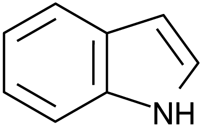
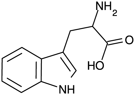
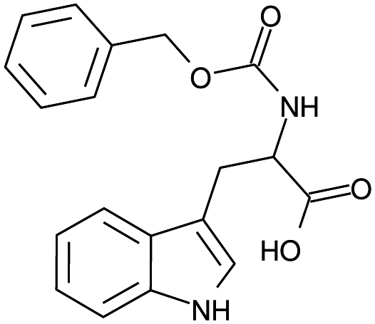
A further advantage of indole is that the naturally occurring, essential amino acid tryptophan and its derivatives contain an indole moiety. Since these indole based amino acids are very abundant in peptides and proteins, this might allow the investigation of biologically relevant systems in the future. In addition, tryptophan and numerous tryptophan derivatives are also commercially available, i.e. without custom synthesis, and there are indications for their suitability as TSD probe34–37,39,43,44 and their likely applicability to biochemical systems.45,46 In order to obtain a reliable statement on its suitability as TSD probe in biochemical investigations, cbz-tryptophan was chosen, since it is interesting whether a phenyl ring in close vicinity to the indole unit influences the triplet state, e.g. through quenching effects. For a better understanding, in Table 1 the structural formula of indole, tryptophan and cbz-tryptophan as well as essential properties of indole are given.
This paper shows an analysis of indole and cbz-tryptophan using absorption and phosphorescence spectra. Based on this, TSD measurements with both candidates in the well understood van der Waals liquid 2-methyltetrahydrofuran (2-MTHF) are discussed. Of particular interest is the relation of indole to the polar dye quinoxaline, and the influence of the scaffold of cbz-tryptophan on TSD measurements. After these investigations the results of indole obtained in the so far also well understood H-bonding liquid 1-propanol are presented. Results of quinoxaline and naphthalene in 2-MTHF used for comparison with indole are shown in the appendix.
2 Experimental section
2.1 Materials
The standard polar TSD probe quinoxaline (QX) was purchased from Alfa Aesar (98+%), while the nonpolar naphthalene (NA) was ordered from Sigma Aldrich (99%). Both TSD probe candidates, indole (≥99%) and cbz-tryptophan (97%) were also purchased from Sigma Aldrich. All of these substances were used as received. The solvents 2-methyltetrahydrofuran (2-MTHF, 99%, stabilized with 150–400 ppm butylated hydroxytoluene) and 1-propanol (99.9%, anhydrous) were both obtained from Alfa Aesar and filtered through a 200 nm syringe filter.2.2 Measurements
For the absorption measurements the solute concentration was 1 × 10⁻⁴ mol mol−1. The measurements were performed at room temperature in the solvent 2-MTHF. The solution was filled into a quartz cell with a layer thickness of 2 mm. Light from a deuterium-halogen-lamp (Ocean Optics, model DH-2000) was guided through an optical fiber to the quartz cell positioned directly in front of the entrance slit of a Czerny–Turner grating spectrograph (Shamrock 500i from Andor Technology) equipped with gratings of 150, 600, 1800 lines per mm.13 The absorption measurements were performed with the 150 lines per mm grating, while the emission spectra for TSD measurements were recorded with the 600 lines per mm grating. For an overview of the whole emission spectrum the 150 lines per mm grating was used.The TSD measurements themselves were performed with a setup described elsewhere in detail.13,14,47 Three different excitation wavelengths (355 nm, 320 nm and 266 nm) are available to excite the TSD probes. The pulse energies were attenuated to ≈2 mJ to prevent the dye molecules from bleaching. Furthermore, the repetition rate flaser of the pulsed laser system has to be adapted to the phosphorescence lifetime τprobe of the dyes so that flaser ≤ 1/(3τprobe) is always guaranteed. The phosphorescence lifetimes of the dye molecules used below the glass transition temperature Tg range from τQX ≈ (0.27–0.31) s10,13,14 over τNA ≈ (2.1–2.5) s10,13,15,48 to τindole,![[thin space (1/6-em)]](https://www.rsc.org/images/entities/char_2009.gif) tryp. ≈ (6.5–7) s.33,35 In all cases τ is found to decrease with increasing temperature.
tryp. ≈ (6.5–7) s.33,35 In all cases τ is found to decrease with increasing temperature.
In order to optimize the overall measurement time for TSD measurements the solute concentration was increased up to maximum 2 × 10⁻⁴ mol mol−1 and the time-resolved phosphorescence emission spectra were recorded in two different ways depending on the lifetimes of the TSD probes. In the case of quinoxaline and naphthalene the time resolution Δt/t was optimized for each decade and each time point was accumulated after a separate excitation. In that way the decreasing emission intensity was compensated. In the case of indole and cbz-tryptophan, however, this method would be very time-consuming (≈(36–72) h per temperature), so only the first decade of time points was recorded in this way. For longer times the spectra at all relevant time delays were recorded after a single laser pulse with a fixed gate width (Δt) of the camera optimized for the shortest delay time of this series. In that way, the information on the intensity is preserved, which can be used to calculate phosphorescence lifetimes by following an established procedure.13,14 The time resolution Δt/t was better than 5% for quinoxaline, better than 8% for naphthalene and better than 10% for indole as well as cbz-tryptophan. In addition, each spectrum consists of at least 1.5 × 10⁶ counts at the peak maximum with the background subtracted.
3 Results and discussion
3.1 Absorption and emission spectra of indole and cbz-tryptophan
Following the procedure outlined above and successfully tested in ref. 13, the first step to check the candidates indole and cbz-tryptophan for their applicability as TSD probes is to determine their absorption spectra and, hence, a suitable excitation wavelength. It is sufficient to determine this at room temperature, since the position of the absorption spectra does not change significantly with decreasing temperature.34,49 However, since it is not mandatory for the TSD application to excite at the wavelength with the highest absorption coefficient anyway, even a slight spectral shift of the absorption spectrum with decreasing temperature would have no significant effect. Fig. 1 shows the solvent-adjusted absorption spectra of indole and cbz-tryptophan compared to quinoxaline (polar) and naphthalene (nonpolar). It is apparent that indole and cbz-tryptophan have a comparable absorption spectrum, the latter being red-shifted by only ≈7 nm, which is irrelevant for the application as TSD probe, and in agreement with literature data.34,37,40 Both absorption spectra are similar to that of naphthalene, so that both molecules can also be excited with the wavelength λ = 266 nm. Furthermore, the absorption coefficient measured for indole in 2-MTHF agrees with the absorption coefficient determined in the literature for various solvents,34,40 suggesting that solvent dependence of the spectrum is similarly weak as for the other TSD probes used so far.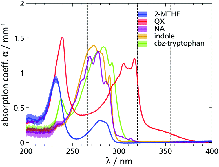 | ||
| Fig. 1 Comparison of the solvent-adjusted absorption spectra of different TSD probes. The absorption coefficient α is plotted against the wavelength λ. The measurements were performed in 2-MTHF at room temperature. The existing excitation wavelengths of the laser system are shown as dashed lines. The data for quinoxaline were taken from the literature.13 It can be seen that the TSD probe candidate indole has an absorption coefficient similar to naphthalene and can be excited with the wavelength λ = 266 nm. | ||
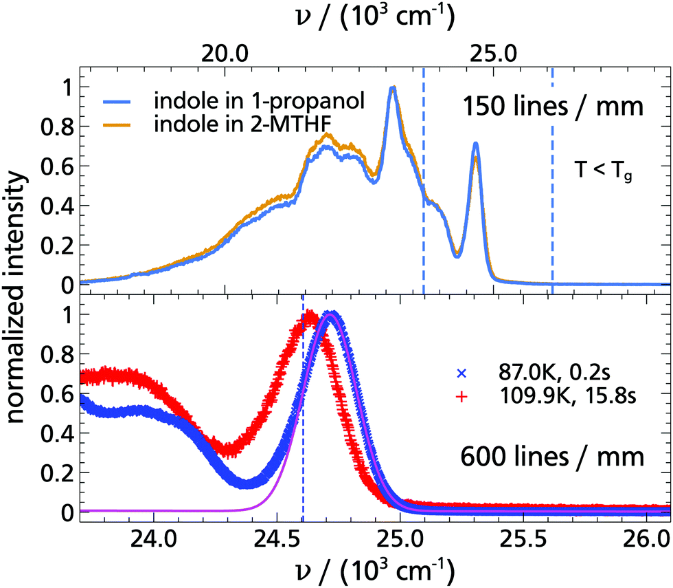
As the next step, the emission spectra of indole and cbz-tryptophan were checked in terms of the quantum yield of the triplet state and whether individual peaks allow the resolution of the time-dependent spectral shift. For that purpose, phosphorescence spectra at two temperatures and delay times were recorded under different conditions as shown in Fig. 2. The mere fact that such spectra can be recorded means that the quantum yield of the triplet state is high enough for the intended purpose, consistent with literature results.33,36,37,50 As shown in Fig. 2 the individual peaks of indole and cbz-tryptophan are sufficiently well resolved and separated to allow for time resolved analysis of a spectral shift of the entire spectrum. Especially, the high energy peak is very suitable, since it is well pronounced and hardly influenced by other spectral features.
 | ||
| Fig. 2 Phosphorescence spectra of indole and cbz-tryptophan in 2-MTHF. The normalized intensity is plotted against the wavenumber ν = 1/λ. The data in the upper part of the figure were recorded with the 150 lines per mm grating while data in the lower part were measured with the 600 lines per mm grating. The spectra for indole and cbz-tryptophan recorded at two different temperatures in the lower part of the figure illustrate the strength of the total spectral shift. In addition, the quantitative evaluation of the spectra is exemplified by the magenta fitting curves. | ||
Furthermore, it can be seen for indole as well as cbz-tryptophan that the spectra are red-shifted with increasing temperature and the total spectral shift is in the order of ≈150 cm−1, consistent with ref. 33, and located between the total Stokes shift of quinoxaline and naphthalene (cf. Appendix A). Thus, both indole and cbz-tryptophan seem to be excellent candidates to be used as TSD probes.
In addition, the spectra of indole and cbz-tryptophan look very similar, despite the fact that the entire spectrum of cbz-tryptophan is red-shifted by ≈300 cm−1 compared to the spectrum of indole. This is a direct consequence of the red-shift of the absorption coefficient, but without further impact on all subsequent evaluations, as was already found for naphthalene and its derivatives.13 Such a fundamental similarity of the spectra and the total spectral shift rather indicate that in cbz-tryptophan the indole unit is the phosphorophore and that this unit is not significantly affected by the phenyl ring of the cbz-protecting (benzyloxycarbonyl) unit.
Since both, indole and cbz-tryptophan, are suitable as TSD probes the questions arises how both perform in solvation measurements, and how the solvation response compares to that of the TSD probes previously available. This is discussed in the following for two solvents, namely for the van der Waals liquid 2-MTHF and the H-bonding liquid 1-propanol. For both solvents the TSD response is quite well understood.9,10,14,15
3.2 Solvation response of indole in the van der Waals liquid 2-MTHF
In order to obtain the so-called solvation response function Csolv.(t) for each TSD probe-solvent combination, the high-energy wing of the phosphorescence spectra is described with a modified Gaussian function‡ (cf.Fig. 2) to obtain the mean energy 〈ν〉 as a function of time and temperature. Compared to the common procedure,10,14 this has the advantage that a nonzero baseline, possibly caused by an excitation of the solvent, can be taken into account, making the description more precise especially for small total spectral shifts and at low temperatures. Csolv.(t) can then be evaluated as: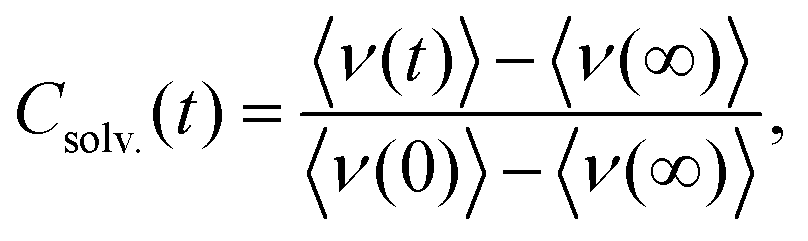 | (1) |
The corresponding solvation response functions Csolv.(t) are presented in Fig. 3 where, in a temperature range from T = 88.0 K to T = 97.0 K, a dynamic range of three orders of magnitude is covered. Particularly noteworthy is the long time behavior which extends up to 15.8 s, due to the longer lifetime of indole compared to the previously used TSD probes.5,9,13,14 The latter is determined at selected temperatures to be τindole(88 K) = (6.55 ± 0.05) s and τindole(94 K) = (5.73 ± 0.11) s, which is in accordance with literature data.35
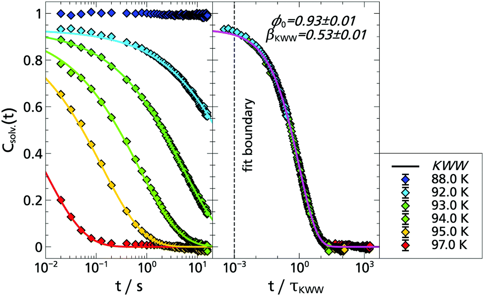 | ||
| Fig. 3 Left: Csolv.(t) of indole in 2-MTHF is plotted against the time t. The KWW functions shown are from the global fit in the masterplot. Right: Masterplot of indole in 2-MTHF, i.e. Csolv.(t) is plotted vs. t/τKWW. Both an α- and a weak β-relaxation process are clearly visible. To describe the α-relaxation process, a KWW function was fitted to the data, which resulted in ϕ0 = 0.93 ± 0.01 and βKWW = 0.53 ± 0.01. The fit range was restricted to the time interval, where the small β-process is of negligible influence. | ||
Typically, solvation response functions are dominated by the α-relaxation process,5,10,14,25,31,51,52 which is usually described by a Kohlrausch–Williams–Watts (KWW) function:
| ϕ(t) = ϕ0·exp[−(t/τKWW)βKWW], | (2) |
Therefore, the question arises how the results obtained with indole compare with previous results, in particular with the polar TSD probe quinoxaline. Thus, Fig. 4 shows a combined data set with both response functions. Without any scaling, the data sets of quinoxaline and indole complement each other perfectly within measurement accuracy. The slight deviations are due to the limited accuracy of the temperature sensors. Thus, by combining the two polar TSD probes, it is now possible to record the solvation response function Csolv.(t) covering five decades in time, with two orders of magnitude of overlap so that a significant extension in time range is achieved. Correspondingly, when comparing the results of the KWW analysis, it turns out that both the α-relaxation and the strength ratio of α- to β-process are identical for both TSD probes (cf. Appendix A).
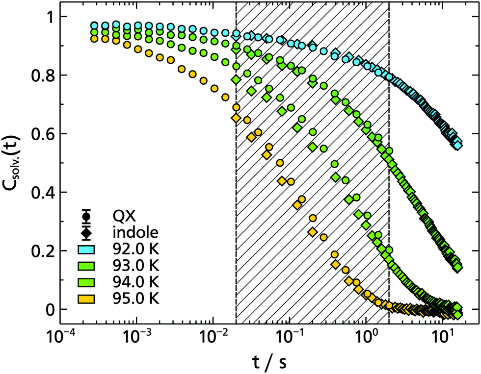 | ||
| Fig. 4 Comparison of the solvation response functions Csolv.(t) measured with indole and quinoxaline in 2-MTHF. The time t is plotted on the abscissa. No scaling was performed. The data sets measured with the two different TSD probes complement each other, so that the combination of both polar probes leads to a time range of five decades in time with an overlap of two orders of magnitude (shaded area). | ||
3.3 Solvation response of cbz-tryptophan in 2-MTHF
Concerning the solvation response, the situation with cbz-tryptophan is expected to be different from the previous case of indole. This is schematically shown in Fig. 5 where the phosphorophore, i.e. the indole unit, is represented in the center. It becomes clear that, besides the solvent molecules, the polar but non phosphorophoric rest will play a role in the first solvation shell around the phosphorophore. Thus, one may expect a significant change in the total spectral shift as well as in the time resolved solvation response. And indeed, evaluation of the total Stokes shift of cbz-tryptophan yields: Δνcbz-tryp. = (156.9 ± 1.7) cm−1 > (135.3 ± 0.8) cm−1 = Δνindole.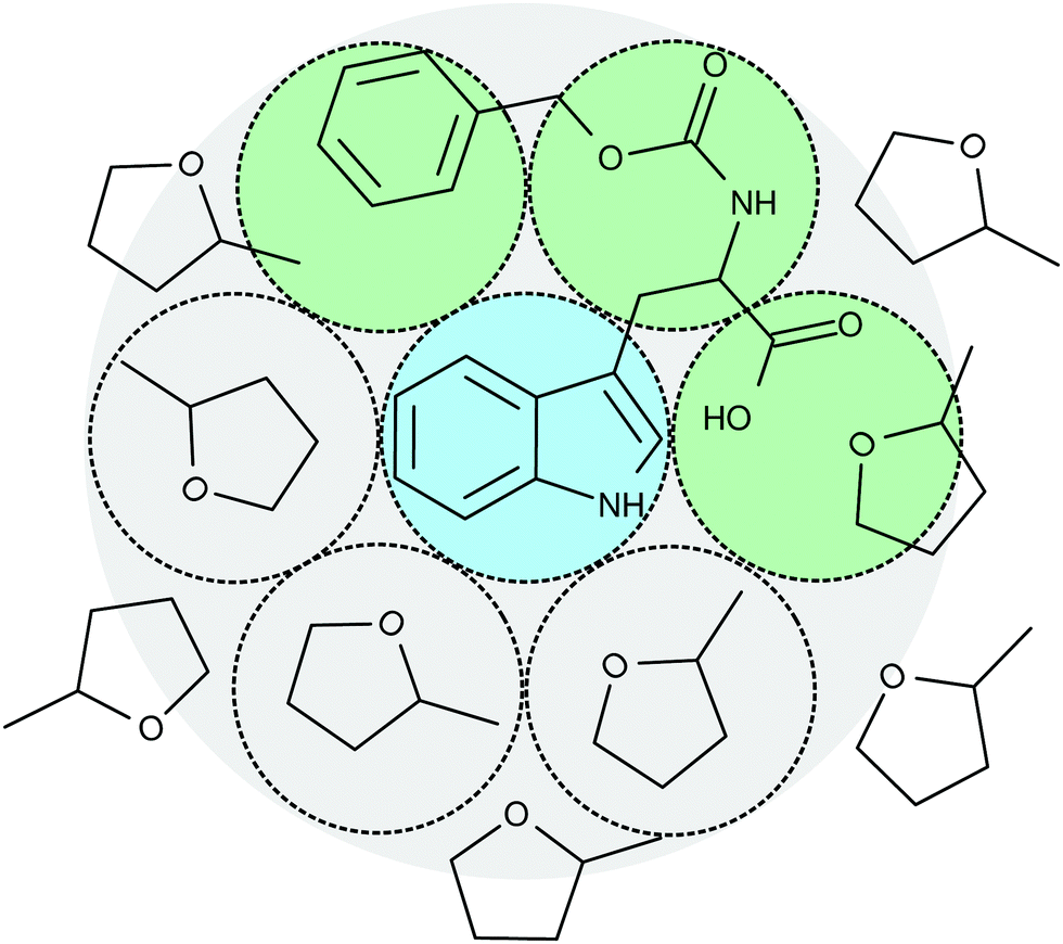 | ||
| Fig. 5 The situation of the solvation measurement of cbz-tryptophan in 2-MTHF schematically shown in 2D. Depicted in the center is the phosphorophore, i.e. the indole unit, whose size is estimated by the blue circle. The first solvation shell is schematically shown in grey. In 3D approximately a dodecahedral arrangement can be expected, in which the non phosphorophoric rest of cbz-tryptophan covers two to three of these spheres (green). | ||
Furthermore, following a rough estimate§ about ≈20% of the solvation response function Csolv.(t) are expected to be due to the non phosphorophoric rest. Moreover, since this rest is larger than the solvent molecules and also subunits cannot move freely, it is likely that the contribution to the solvation response function Csolv.(t) is slower than the reorientation of the solvent molecules and thus should appear as a second process at longer times. In addition, the reorientation of the solvent molecules close to cbz-tryptophan might be slowed down compared to the smaller indole or quinoxaline. However, since this does not affect all solvent molecules in an equal manner and the influence of the scaffold may also be slightly different depending on its orientation in different configurations, the dynamic heterogeneity may also increase.
To some extent these expectations can be checked by comparing the solvation response functions Csolv.(t) for cbz-tryptophan with those of indole, quinoxaline and naphthalene, all in 2-MTHF (for details on quinoxaline and naphthalene data, see Appendix A). For that purpose Csolv.(t) for each respective TSD probe is scaled onto the respective curve at T = 95 K, assuming time-temperature superposition (TTS) to be valid at least for the α-relaxation. The resulting comparison is shown in Fig. 6. It shows that the dynamics in 2-MTHF measured with cbz-tryptophan is indeed slower than the dynamics measured with the other TSD probes and shows a second process at long times, whose contribution in the total decrease of the solvation response is roughly within the estimated ≈20%.
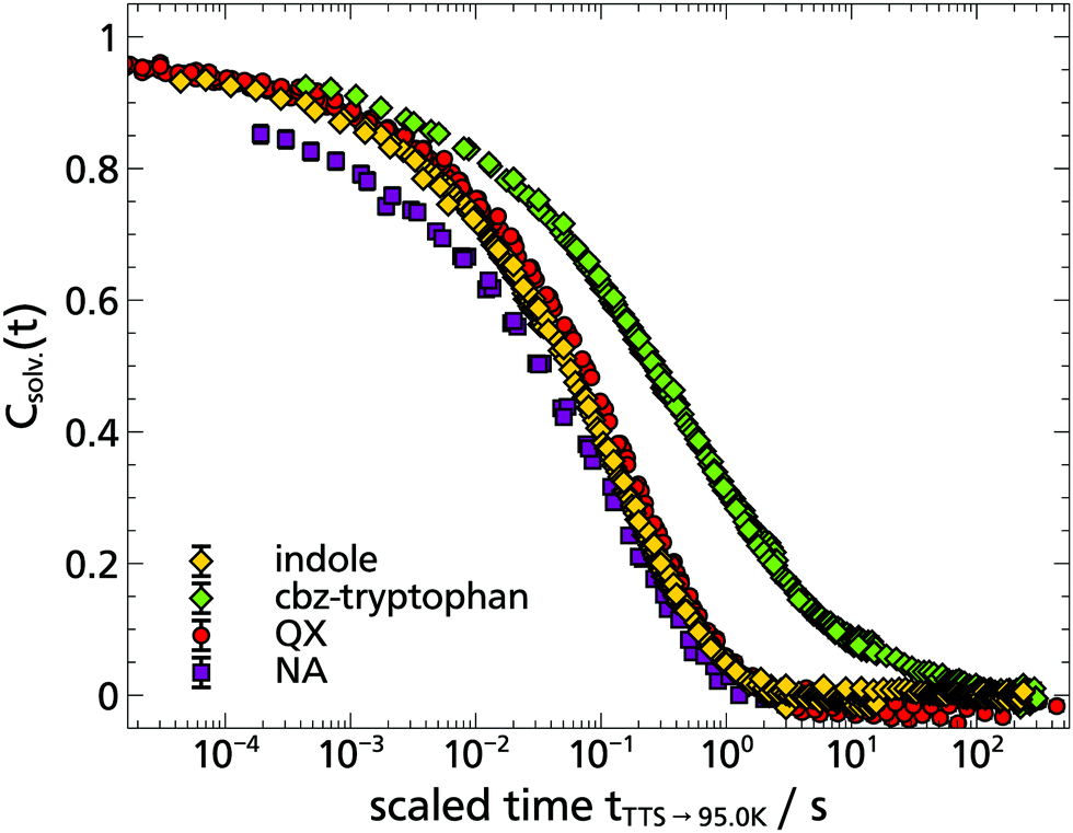 | ||
| Fig. 6 Comparison of the solvation response of the TSD probes indole, cbz-tryptophan, quinoxaline and naphthalene in 2-MTHF. The time-temperature superposition (TTS) of the respective solvation response functions Csolv.(t) is plotted onto the respective curve for 95.0 K. | ||
To allow for a more quantitative comparison, the curve of cbz-tryptophan shown in Fig. 6 was fitted with a sum of two KWW functions eqn (2), ϕ1(t) to describe the relaxation process of the solvent molecules and ϕ2(t) the relaxation of the scaffold, respectively. As both relaxation contributions overlap strongly, decent starting values or boundary conditions are required. Therefore τ1 < τ2, 0.9 ≤ ϕ0,1 + ϕ0,2 ≤ 1 and from above considerations ϕ0,2 ≈ 0.2 applies. Furthermore, it has been shown for TSD data that in many cases
| βKWW ≈ 0.5 | (3) |
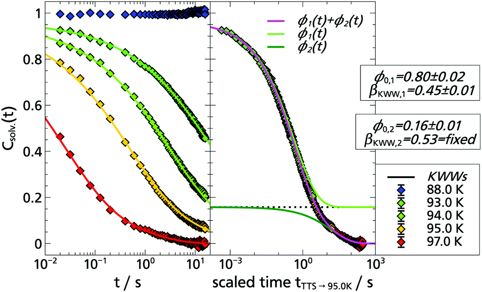 | ||
| Fig. 7 Left: Csolv.(t) of cbz-tryptophan in 2-MTHF is plotted against the time t. The shown KWW functions result from the global fit (see right). Right: Time–temperature superposition (TTS) applied to cbz-tryptophan solvation response functions Csolv.(t) scaling all curves onto the 95.0 K decay. Solid lines indicate the composition of the fit. Parameters are indicated in the figure. See text for details. | ||
Based on the fit results and the comparison of the time constants obtained in 2-MTHF with different TSD probes (cf. Arrhenius plot Fig. 8), several conclusions can be drawn. First, although hard to separate unambiguously, two relaxation processes can be distinguished, the faster process being due to the relaxation of the solvent molecules and the slower process being due to the relaxation of the non phosphorophoric rest of the cbz-tryptophan, supporting the simple picture sketched in Fig. 5. Second, the non phosphorophoric rest of the cbz-tryptophan increases the dynamic heterogeneity and slows down the reorientation dynamics of the solvent compared to indole and the other smaller TSD probes, most probably due to the steric restrictions of the scaffold.
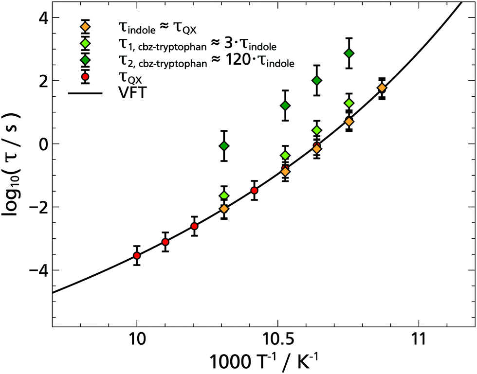 | ||
| Fig. 8 Arrhenius plot of relaxations times from the solvation response in the glass-former 2-MTHF. The logarithmic relaxation times are plotted against the inverse temperature. The TSD results obtained with different probes and a Vogel–Fulcher–Tammann function (solid line) is shown, which is adapted to the quinoxaline data. The latter are in agreement with TSD data and also dielectric data from the literature.5 | ||
Another point to be mentioned is that the temperature-dependent phosphorescence lifetime differs only slightly between cbz-tryptophan and indole. Following the same procedure as for indole, the lifetime can be determined for a few temperatures as τcbz-tryp.(88 K) = (6.19 ± 0.01) s and τcbz-tryp.(94 K) = (5.53 ± 0.09) s, which is in accordance with data obtained for tryptophan in the literature.35 From these findings, it can be concluded that a conceivable phosphorescence quenching caused by the phenyl ring – which in cbz-tryptophan is very close to the phosphorophore – plays at best a minor role. This is an important finding with regard to further applicability of tryptophan and its derivatives.
Thus, also a tryptophan derivative can be used to study local solvation dynamics, with the indole unit being the only phosphorophore, which is analogous to the results obtained with naphthalene derivatives.13
3.4 Solvation response of indole in the H-bonding liquid 1-propanol
In order to study indole in a hydrogen bonding solvent, the monohydroxy alcohol 1-propanol was chosen, as a solvent which is already well investigated with TSD. In addition, the dipolar and mechanical solvation in 1-propanol are also well separated, so that possible differences between the TSD probes indole, quinoxaline and naphthalene become more obvious.9,14,15The phosphorescence spectra of indole in 1-propanol are compared with those in 2-MTHF in Fig. 9. Obviously, the spectra of indole have a negligible dependence on the solvent and the total Stokes shift of indole has the same order of magnitude in both cases, yielding for 1-propanol: Δν = (90.1 ± 1.4) cm−1. In comparison, the spectral shift in 1-propanol measured with indole is considerably smaller than the one obtained with quinoaxaline (ΔνQX = (551 ± 10) cm−1),14 but has the same order of magnitude as the one obtained with the nonpolar TSD probe naphthalene in the same solvent (ΔνNA = (60.9 ± 2.2) cm−1).15
 | ||
| Fig. 9 Phosphorescence spectra of indole in 1-propanol compared to those in 2-MTHF. The normalized intensity is plotted against the wavenumber ν = 1/λ. The data in the upper part of the figure were recorded with the 150 lines per mm grating while the data in the lower part were measured with the 600 lines per mm grating. The spectra of indole in 1-propanol recorded at two different temperatures in the lower part of the figure illustrate the strength of the total spectral shift. In addition, the quantitative evaluation of the spectra is exemplified by the magenta fitting curves. | ||
The solvation response functions of indole in 1-propanol are shown in Fig. 10. The KWW analysis applied to the master curve yields ϕ0 = 0.71 ± 0.02 and βKWW = 0.50 ± 0.01, with the stretching parameter being in the typical range for the α-relaxation process and being identical within experimental uncertainty with the values determined with quinoxaline and naphthalene in 1-propanol.14,15 Although the ϕ0 value is more difficult to determine accurately, a comparison between the TSD probes yields ϕ0,QX > ϕ0,indole > ϕ0,NA, which means that the strength of the β-relaxation contribution for indole in 1-propanol lies in between that of quinoxaline and naphthalene.
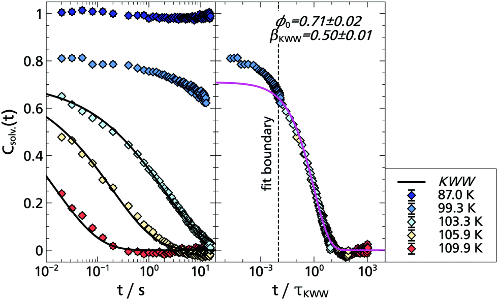 | ||
| Fig. 10 Left: Csolv.(t) of indole in 1-propanol is plotted against the time t. The KWW functions shown result from the global fitting in the masterplot. Right: Masterplot of indole in 1-propanol, i.e. Csolv.(t) is plotted vs. t/τKWW. Both an α- and β-relaxation process are clearly visible. To describe the α-relaxation process, a KWW function was fitted to the data, which resulted in ϕ0 = 0.71 ± 0.02 and βKWW = 0.50 ± 0.01. The fit boundary was chosen such that the α-relaxation process can be described as independently as possible from the β-relaxation process. | ||
In Fig. 11 a comparison of three different TSD probes indole, quinoxaline and naphthalene is shown by applying TTS to the α-process and scaling all curves onto the respective solvation response at T = 109.9 K. Obviously, the timescale of the solvation response for indole lies in between that of the dipolar quinoxaline and the non-polar naphthalene. This can be understood considering that each polar TSD probe not only measures the dipolar solvation, but also a contribution of the mechanical solvation,9 which can be separately accessed with a non-polar dye like naphthalene. Assuming that the mechanical solvation contribution approximately has the same amplitude for all three probe molecules, the indole response would contain a greater contribution of mechanical solvation than quinoxaline. For indole in 1-propanol this contribution of mechanical solvation can be estimated as Δνmech/Δνmech+dipol = ΔνNA/ΔνIndol ≈ 68%, while for quinoxaline it is approximately ΔνNA/ΔνQX ≈ 11%. In contrast to 2-MTHF,2 where the timescales of dipolar and mechanical solvation are almost identical, they are generally well separated in monohydroxy alcohols,53–55 and in particular in 1-propanol.14,15 Thus, the solvation response of indole is the result of the particular weighting of mechanical and dipolar solvation in this TSD probe: this is demonstrated by the dashed line in Fig. 11, which is a superposition of the fits shown for quinoxaline and naphthalene weighted by the total spectral shift according to the above considerations, i.e., ϕindole(t) = 0.32·ϕQX(t) + 0.68·ϕNA(t), approximately assuming ϕQX(t) to represent the dipolar and ϕNA(t) to represent the mechanical solvation response, respectively. Despite the approximate nature of this reasoning the superposition (blue dashed line) reproduces the indole response function rather well, without further fit parameters. A similar argument holds concerning the relative amplitude of the β-relaxation, which is known to be extraordinarily strong in the macroscopic shear mechanical response of 1-propanol, much stronger than in the dielectric loss.15 Accordingly, the β-process contribution in indole lies between that of naphthalene and quinoxaline, as described above.
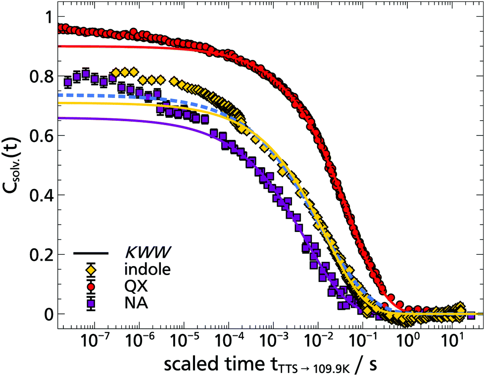 | ||
| Fig. 11 Comparison of the TSD probes indole, quinoxaline and naphthalene in 1-propanol. The time–temperature superposition (TTS) of the respective solvation response functions Csolv.(t) is plotted onto 109.9 K. In addition, the corresponding KWW functions are shown as solid lines,14,15 while the dashed blue line represents an superposition of the quinoxaline and naphthalene KWW functions weighted by the total Stokes shift to describe the indole data. | ||
Thus, it becomes clear, why a simple merging of the data, as was successful for 2-MTHF (cf.Fig. 6), cannot work for 1-propanol: both, a different relative β-process contribution and a different timescale of local mechanical and dipolar response contributions hamper a simple merging of the data. However, if the different relative α-relaxation amplitudes are normalized by scaling out the corresponding ϕ0, it becomes obvious that the different weighting of mechanical and dipolar solvation in the response of each TSD probe boils down to a difference in timescale. As Fig. 12 shows, the indole response function decays faster by a factor 4 compared to the one of quinoxaline, while at the same time it is slower by a factor of 3 than the mechanical solvation response measured with naphthalene, while to good approximation the line shape is maintained. Whenever this condition is fulfilled, the data sets of different TSD probes can be combined in a suitable way so that local dielectric and mechanical solvation dynamics are accessible covering up to five orders of magnitude in time.
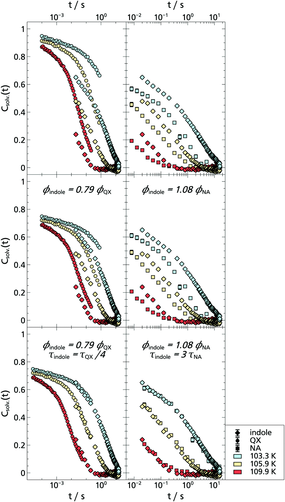 | ||
| Fig. 12 Comparison of the solvation response functions Csolv.(t) measured with indole in 1-propanol with the results obtained for quinoxaline (left) and naphthalene (right). The time t is plotted on the abscissa. Upper figures: No scaling is applied. The data sets measured with the different TSD probes do not seem to complement each other, but rather reflect different dynamic aspects. Middle figures: The different relative strengths of the α/β-relaxation processes of the respective TSD probes are scaled out using the corresponding ϕ0 parameters. Lower figures: Now also the relaxation times are rescaled: apparently, the response function of indole decays faster by a factor of 4 than the one of quinoxaline, but at the same time slower by a factor of 3 than the response of naphthalene. | ||
4 Summary and conclusion
In summary, it was shown that indole and its derivative cbz-tryptophan can be used as TSD probes and thus extend the dynamic range used so far to cover longer timescales. It turns out that to a good approximation indole is the phosphorophore in cbz-tryptophan and that the phenyl ring, which is very close to it plays at best a minor role regarding a negative impact on solvation measurements. The former observation is in line with the results previously obtained with naphthalene modifications. Based on the data available to date, it can therefore be expected that such TSD probe modifications can be generalized and follow a certain pattern. The remaining, non phosphorophoric rest has, on the one hand a non-negligible influence on the reorientation of the solvent molecules. On the other hand, by itself it contributes to the solvation response function Csolv.(t), which can be rationalized by a simple model.Moreover, indole was characterized in two well investigated solvents, namely the van der Waals liquid 2-MTHF and the hydrogen bonding liquid 1-propanol. It was found that due to the different change in dipole moment on excitation the total spectral shifts are related as ΔνQX > Δνindole > ΔνNA. As a result, the solvation response of the polar TSD probe indole contains a larger contribution of the mechanical solvation than the likewise polar quinoxaline, regardless of whether a van der Waals or an H-bonding solvent is probed. In both cases, the contribution of the measured mechanical solvation accounts for ≈2/3 of the total solvation response (cf. also Appendix A). This in turn means that in a solvent such as 2-MTHF, in which the mechanical hardly differs from the dipolar solvation response, the data sets measured with indole and quinoxaline can be combined without any further scaling, thus covering a measurement window of five decades. If, on the other hand, the mechanical solvation response differs significantly from the dipolar one, as in the case of monohydroxy alcohols, the different contributions of mechanical and dipolar solvation for each TSD probe lead to apparent differences in the response functions. However, as these hardly affect the overall line shape, these differences can be accounted for and thus, effectively a combination of data sets becomes possible again.
This fundamental understanding of indole based TSD probes will allow its use also for investigating biologically relevant processes in the future. By recording temperature- and time-dependent phosphorescence spectra, the TSD technique can provide insights into the reorientation dynamics of solvent molecules and thus complement the phosphorescence-based methods used so far,38–40,43–46 especially in the supercooled regime.
Conflicts of interest
There are no conflicts to declare.Appendix A 2-MTHF investigated by the standard TSD probes quinoxaline and naphthalene
Due to the fact that the van der Waals liquid 2-MTHF is a quite fragile solvent (fragility index of ≈65)56 comparatively small temperature changes have quite an impact on the dynamics. Therefore, 2-MTHF was investigated by the standard TSD probes quinoxaline (polar, i.e., reflecting mainly the dipolar solvation) and naphthalene (nonpolar, i.e., reflecting mechanical solvation) with the same setup that is used for the TSD measurement presented in this paper to minimize temperature offsets. Furthermore, due to an improved setup the data presented here extend the data shown in the literature.2,10 In Fig. 13 the solvation response function Csolv.(t) of the polar TSD probe quinoxaline in 2-MTHF measured over a dynamic range of four orders of magnitude in the temperature range from 88.0 K up to 100.0 K is shown. Data evaluation proceeds in the same way as presented above. The total Stokes shift was calculated as ΔνQX = (254.8 ± 3.2) cm−1 and is thus larger than the one of indole. As indicated in the figure the extension of the measuring window to shorter times clearly reveals a small β-relaxation contribution in 2-MTHF. Otherwise, within the uncertainty limits of the temperature measurements, the data shown here are in agreement with the data presented in the literature.52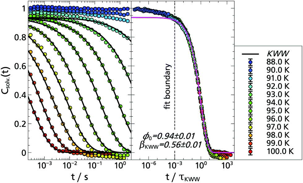 | ||
| Fig. 13 Left: Csolv.(t) of quinoxaline in 2-MTHF is plotted against the time t. The KWW functions shown are from the global fit in the masterplot. Right: Masterplot of quinoxaline in 2-MTHF, i.e. Csolv.(t) is plotted vs. t/τKWW. Both an α- and a weak β-relaxation process are clearly visible. The α-relaxation process is described with a KWW function with ϕ0 = 0.94 ± 0.01 and βKWW = 0.56 ± 0.01. The fit limits were chosen such that the α-process is described approximately independent from the weak β-relaxation. | ||
The solvation response functions Csolv.(t) of the nonpolar TSD probe naphthalene in 2-MTHF are presented in Fig. 14, where in the temperature range from 88.0 K up to 100.0 K a dynamic range of three orders of magnitude is covered. The data are in agreement with the fixed-lagtime temperature scan presented in the literature.2,10 Applying the same data analysis as before, leads to a slightly larger β-process contribution to Csolv.(t) compared to quinoxaline and an total spectral shift of ΔνNA = (88.0 ± 1.4) cm−1. By assuming that the mechanical solvation response approximately has the same amplitude for the three TSD probes indole, quinoxaline and naphthalene it can be estimated that the solvation response of indole contains a larger contribution of mechanical solvation than quinoxaline: Δνmech/Δνmech+dipol = ΔνNA/Δνindole ≈ 65% in contrast to ΔνNA/ΔνQX ≈ 35%.
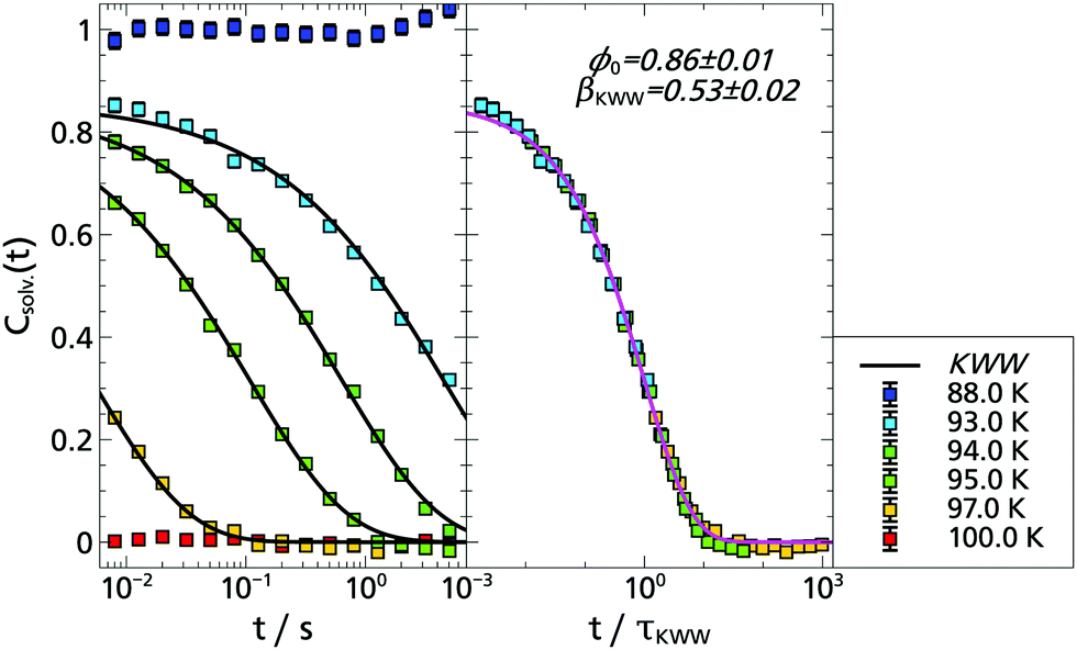 | ||
| Fig. 14 Left: Csolv.(t) of naphthalene in 2-MTHF is plotted against the time t. The KWW functions shown are from the global fit in the masterplot. Right: Masterplot of naphthalene in 2-MTHF, i.e. Csolv.(t) is plotted vs. t/τKWW. Both an α- and a weak β-relaxation are clearly visible. To describe the α-relaxation, a KWW function, was fitted to the data, which resulted in ϕ0 = 0.86 ± 0.01 and βKWW = 0.53 ± 0.02. The fit limits were chosen the same as above for quinoxaline. | ||
However, due to the fact that in 2-MTHF, in contrast to 1-propanol,9,15 mechanical and dipolar solvation do not differ significantly in timescale, shape or in the strength of the β-relaxation contribution,2 this finding does not lead to a significant difference in the solvation response functions of the respective TSD probes. As indicated in Fig. 15 only a minor scaling has to be applied to merge Csolv.(t) measured with naphthalene and quinoxaline in 2-MTHF, which is in accordance with previous findings.2
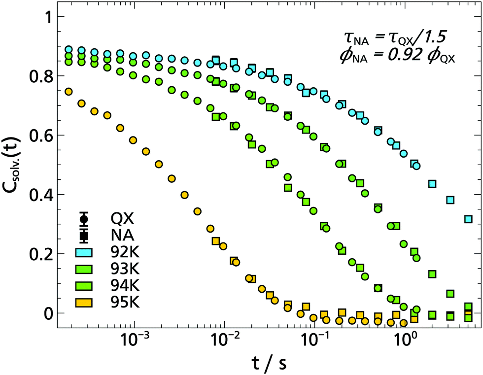 | ||
| Fig. 15 Comparison of the solvation response functions Csolv.(t) measured with naphthalene and quinoxaline in 2-MTHF. The time t is plotted on the abscissa. Only a minor scaling was applied to the data as indicated in the figure. | ||
Finally, Fig. 16 shows the Arrhenius plot of 2-MTHF, in which only the measured data of the two standard TSD probes quinoxaline and naphthalene is contained, as these points are partially covered in Fig. 8. A Vogel–Fulcher–Tammann (VFT) description to the quinoxaline data is also applied and compared to the description given in the literature.5 The discrepancy of ΔT = 0.3 K can be attributed to the uncertainty of the temperature measurement.
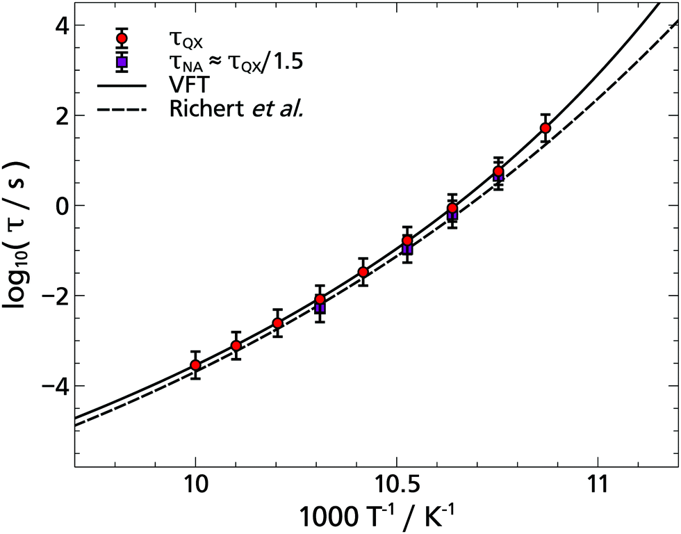 | ||
| Fig. 16 Arrhenius plot of the glass-former 2-MTHF. The logarithmic relaxation times from the solvation response obtained with quinoxaline and naphthalene are plotted against the inverse temperature. In addition, a Vogel–Fulcher–Tammann function (VFT) is fitted to the quinoxaline data, which is in agreement with the literature and dielectric time constants is shown.5 | ||
Acknowledgements
Financial support of this work by the Deutsche Forschungsgemeinschaft (DFG) in the framework of the research unit FOR 1583 under Grant No. BL1192/1 and No. TH1115/8-1 is gratefully acknowledged.References
- M. Maroncelli, J. MacInnes and G. R. Fleming, Science, 1989, 243, 1674–1681 CrossRef CAS PubMed.
- R. Richert and A. Wagener, J. Phys. Chem., 1991, 95, 10115–10123 CrossRef CAS.
- M. Maroncelli, J. Mol. Liq., 1993, 57, 1–37 CrossRef CAS.
- J. T. Fourkas, A. Benigno and M. Berg, J. Chem. Phys., 1993, 99, 8552–8558 CrossRef CAS.
- R. Richert, F. Stickel, R. Fee and M. Maroncelli, Chem. Phys. Lett., 1994, 229, 302–308 CrossRef CAS.
- J. Ma, D. V. Bout and M. Berg, J. Chem. Phys., 1995, 103, 9146–9160 CrossRef CAS.
- M. Horng, J. Gardecki, A. Papazyan and M. Maroncelli, J. Phys. Chem., 1995, 99, 17311–17337 CrossRef CAS.
- M. Berg, J. Phys. Chem. A, 1998, 102, 17–30 CrossRef CAS.
- H. Wendt and R. Richert, J. Phys. Chem. A, 1998, 102, 5775–5781 CrossRef CAS.
- R. Richert, J. Chem. Phys., 2000, 113, 8404 CrossRef CAS.
- C. Reichardt and T. Welton, Solvents and Solvent Effects in Organic Chemistry, Wiley-VCH Verlag GmbH & Co. KGaA, 2010 Search PubMed.
- C. Allolio, M. Sajadi, N. P. Ernsting and D. Sebastiani, Angew. Chem., Int. Ed., 2013, 52, 1813–1816 CrossRef CAS PubMed.
- P. Weigl, V. Talluto, T. Walther and T. Blochowicz, Z. Phys. Chem., 2018, 232, 1017–1039 CrossRef CAS.
- P. Weigl, D. Koestel, F. Pabst, J. P. Gabriel, T. Walther and T. Blochowicz, Phys. Chem. Chem. Phys., 2019, 21, 24778–24786 RSC.
- P. Weigl, T. Hecksher, J. Dyre, T. Walther and T. Blochowicz, submitted.
- A. S. F. Kremer, Broadband Dielectric Spectroscopy, Springer, Berlin, Heidelberg, 2002 Search PubMed.
- H. Barnes, A handbook of elementary rheology, University of Wales, Institute of Non-Newtonian Fluid Mechanics, Aberystwyth, 2000 Search PubMed.
- B. J. Berne and R. Pecora, Dynamic Light Scattering: With Applications to Chemistry, Biology, and Physics (Dover Books on Physics), Dover Publications, unabridged edn, 2000 Search PubMed.
- T. Blochowicz, A. Brodin and E. A. Rössler, Adv. Chem. Phys., 2006, 133, 127–256 CAS.
- J. Gabriel, F. Pabst, T. Helbling, T. Böhmer and T. Blochowicz, The Scaling of Relaxation Processes, Springer, 2018, pp. 203–245 Search PubMed.
- J. P. Gabriel, P. Zourchang, F. Pabst, A. Helbling, P. Weigl, T. Böhmer and T. Blochowicz, Phys. Chem. Chem. Phys., 2020, 22, 11644–11651 RSC.
- R. Richert, J. Phys.: Condens. Matter, 1996, 8, 6185–6190 CrossRef CAS.
- J. T. Edward, J. Chem. Educ., 1970, 47, 261 CrossRef CAS.
- S. E. Braslavsky, Pure Appl. Chem., 2007, 79, 293–465 CAS.
- R. Richert, Chem. Phys. Lett., 1990, 171, 222–228 CrossRef CAS.
- R. Richert, Chem. Phys. Lett., 1992, 199, 355–359 CrossRef CAS.
- R. Richert and M. Yang, J. Phys.: Condens. Matter, 2003, 15, S1041 CrossRef CAS.
- R. Richert and M. Yang, J. Phys. Chem. B, 2003, 107, 895–898 CrossRef CAS.
- F. He and R. Richert, Phys. Rev. B: Condens. Matter Mater. Phys., 2006, 74, 014201 CrossRef.
- W. Wen and R. Richert, J. Chem. Phys., 2009, 131, 084710 CrossRef PubMed.
- D. Sauer, B. Schuster, M. Rosenstihl, S. Schneider, V. Talluto, T. Walther, T. Blochowicz, B. Stühn and M. Vogel, J. Chem. Phys., 2014, 140, 114503 CrossRef CAS PubMed.
- M. Lannert, A. Müller, E. Gouirand, V. Talluto, M. Rosenstihl, T. Walther, B. Stühn, T. Blochowicz and M. Vogel, J. Chem. Phys., 2016, 145, 234511 CrossRef PubMed.
- W. C. Galley and R. M. Purkey, Proc. Natl. Acad. Sci. U. S. A., 1970, 67, 1116–1121 CrossRef CAS PubMed.
- E. H. Strickland, J. Horwitz and C. Billups, Biochemistry, 1970, 9, 4914–4921 CrossRef CAS PubMed.
- G. B. Strambini and M. Gonnelli, Chem. Phys. Lett., 1985, 115, 196–200 CrossRef CAS.
- R. Klein, I. Tatischeff, M. Bazin and R. Santus, J. Phys. Chem., 1981, 85, 670–677 CrossRef CAS.
- D. Creed, Photochem. Photobiol., 1984, 39, 537–562 CrossRef CAS.
- C. J. Fischer, A. Gafni, D. G. Steel and J. A. Schauerte, J. Am. Chem. Soc., 2002, 124, 10359–10366 CrossRef CAS PubMed.
- G. B. Strambini, B. A. Kerwin, B. D. Mason and M. Gonnelli, Photochem. Photobiol., 2004, 80, 462–470 CrossRef CAS PubMed.
- J. Chavez, L. Ceresa, E. Kitchner, J. Kimball, T. Shtoyko, R. Fudala, J. Borejdo, Z. Gryczynski and I. Gryczynski, J. Photochem. Photobiol., B, 2020, 208, 111897 CrossRef CAS PubMed.
- L. S. Slater and P. R. Callis, J. Phys. Chem., 1995, 99, 8572–8581 CrossRef CAS.
- D. K. Hahn and P. R. Callis, J. Phys. Chem. A, 1997, 101, 2686–2691 CrossRef CAS.
- M. Gonnelli and G. B. Strambini, Biochemistry, 1995, 34, 13847–13857 CrossRef CAS PubMed.
- G. B. Strambini and M. Gonnelli, J. Am. Chem. Soc., 1995, 117, 7646–7651 CrossRef CAS.
- J. M. Vanderkooi and J. W. Berger, Biochim. Biophys. Acta, Bioenerg., 1989, 976, 1–27 CrossRef CAS.
- S. D’Auria, M. Staiano, A. Varriale, M. Gonnelli, A. Marabotti, M. Rossi and G. B. Strambini, J. Proteome Res., 2008, 7, 1151–1158 CrossRef PubMed.
- V. Talluto, T. Blochowicz and T. Walther, Appl. Phys. B: Lasers Opt., 2016, 122, 132 CrossRef.
- W. E. Graves, R. H. Hofeldt and S. P. McGlynn, J. Chem. Phys., 1972, 56, 1309–1314 CrossRef CAS.
- E. H. Strickland, M. Wilchek, J. Horwitz and C. Billups, J. Biol. Chem., 1970, 245, 4168–4177 CrossRef CAS.
- S. Freed and W. Salmre, Science, 1958, 128, 1341–1342 CrossRef CAS.
- H. Wagner and R. Richert, J. Non-Cryst. Solids, 1998, 242, 19–24 CrossRef CAS.
- H. Wendt and R. Richert, Phys. Rev. E: Stat. Phys., Plasmas, Fluids, Relat. Interdiscip. Top., 2000, 61, 1722 CrossRef CAS PubMed.
- B. Jakobsen, K. Niss and N. B. Olsen, J. Chem. Phys., 2005, 123, 234511 CrossRef PubMed.
- B. Jakobsen, C. Maggi, T. Christensen and J. C. Dyre, J. Chem. Phys., 2008, 129, 184502 CrossRef PubMed.
- C. Gainaru, T. Hecksher, N. B. Olsen, R. Böhmer and J. C. Dyre, J. Chem. Phys., 2012, 137, 064508 CrossRef PubMed.
- L.-M. Wang, C. A. Angell and R. Richert, J. Chem. Phys., 2006, 125, 074505 CrossRef PubMed.
Footnotes |
| † It should be noted that the term “Stokes shift” strictly speaking denotes the difference in the spectral position of the Frank–Condon maxima of lowest energy absorption and luminescence resulting from the same electronic transition.24 But since the S0 ← T1(0–0) transition is considered in the present case, it is strictly speaking not a Stokes shift, but a solvation induced shift of the triplet emission spectrum. However, since the term has become established in the description of TSD experiments,10,13,25 it is used here together with the more appropriate synonym “spectral shift” for reasons of consistency with the previous literature on TSD. |
| ‡ I(ν) = a·exp[−(ν − 〈ν〉)2/2σ2] + m·ν + b, where a is the amplitude of the normalized high-energy wing, 〈ν〉 is the mean energy, σ is the optical linewidth and m as well as b describe the linear baseline. |
| § Simply counting the spheres based on Fig. 5 assuming a dodecahedral local structure around the phosphorophore, i.e. the indole unit, yields 2 spheres/12 spheres ≈ 17% or 3 spheres/12 spheres ≈ 25%. |
| This journal is © the Owner Societies 2021 |