 Open Access Article
Towards efficient discovery of green synthetic pathways with Monte Carlo tree search and reinforcement learning†
Xiaoxue
Wang
 ac,
Yujie
Qian
b,
Hanyu
Gao
 a,
Connor W.
Coley
 a,
Yiming
Mo
 a,
Regina
Barzilay
b and
Klavs F.
Jensen
 *a
*a
aDepartment of Chemical Engineering, Massachusetts Institute of Technology, Cambridge, Massachusetts 02139, USA. E-mail: kfjensen@mit.edu
bDepartment of Electrical Engineering and Computer Science, Massachusetts Institute of Technology, Cambridge, Massachusetts 02139, USA
cDepartment of Chemical and Biomolecular Engineering, The Ohio State University, Columbus, Ohio 43210, USA
First published on 14th September 2020
Abstract
Computer aided synthesis planning of synthetic pathways with green process conditions has become of increasing importance in organic chemistry, but the large search space inherent in synthesis planning and the difficulty in predicting reaction conditions make it a significant challenge. We introduce a new Monte Carlo Tree Search (MCTS) variant that promotes balance between exploration and exploitation across the synthesis space. Together with a value network trained from reinforcement learning and a solvent-prediction neural network, our algorithm is comparable to the best MCTS variant (PUCT, similar to Google's Alpha Go) in finding valid synthesis pathways within a fixed searching time, and superior in identifying shorter routes with greener solvents under the same search conditions. In addition, with the same root compound visit count, our algorithm outperforms the PUCT MCTS by 16% in terms of determining successful routes. Overall the success rate is improved by 19.7% compared to the upper confidence bound applied to trees (UCT) MCTS method. Moreover, we improve 71.4% of the routes proposed by the PUCT MCTS variant in pathway length and choices of green solvents. The approach generally enables including Green Chemistry considerations in computer aided synthesis planning with potential applications in process development for fine chemicals or pharmaceuticals.
Introduction
The goal of computer aided synthesis planning (CASP) has traditionally been to identify synthesis pathways to desired compounds from buyable building-block chemicals through retrosynthesis.1–8 Retrosynthetic analysis is a procedure in which a target molecule is broken into precursors recursively until all precursors are commercially available (success) or the process reaches the termination criteria (failure).1–3,9,10 The idea of reaction codification and CASP was introduced in Vléduts's visionary paper in 1963.11 Ever since the first logical retrosynthetic route planning based on a computer program demonstrated by Corey et al.6 in the 1960s, the field of CASP has been evolving rapidly along with the development of large comprehensive reaction databases.4 As examples, Synthia (formerly Chematica), has successfully designed synthesis routes for many medicinally important targets,5,9,12–16 and Coley et al. has demonstrated that with expert chemistry input CASP synthetic routes can be translated successfully into recipes for execution on a robotic platform.17 Existing CASP programs have primarily focused on the success rate1 and the chemical diversity of routes,2,9 but rarely have taken Green Chemistry principles into considerations, e.g., routes with shortest possible length using less toxic and flammable solvents.18,19 However, it is becoming increasingly important to select routes that conform to green chemistry requirement in addition to finding synthetic pathways to buyable starting compounds.One major challenge for an efficient CASP algorithm to include green chemistry considerations is limitations in chemical space search algorithms. The search algorithm is the core of synthesis planning as it determines the success rate and the route quality of the proposed synthesis pathways. Heuristic best first searches (BFS) or depth first searches (DFS)5 use hand-written heuristic functions to evaluate positions in the search tree as they explore the synthesis planning search space.1,5 However, given the large search space5,20 of chemical reactions, the searching efficiency of BFS/DFS is not high enough for good CASP performance.5 In addition, it is difficult to define strong heuristics for BFS/DFS CASP.1 To tackle this challenge, Segler et al.1 showed that Monte Carlo Tree Search (MCTS), a search scheme that demonstrated superhuman performance in playing the game of Go,21,22 is able to find buyable pathways with much higher success rate than traditional heuristic BFS.1 Segler et al.1,23,24 also innovatively demonstrated that it was possible to learn the rules of chemical synthesis for a specific domain by using data. Additionally, Kishimoto et al.25 demonstrated that the MCTS variant used by Segler et al.1 significantly outperformed depth-first proof-number (DFPN) search in terms of success rate in the domain of retrosynthesis. More recently, Chen et al.26 introduced Retro*, a neural-based tree search method also demonstrating advanced performance.
The MCTS variant used by Segler et al. is similar to Google's Alpha Go algorithm.22 Though it has great search success rate, the method does not take green chemistry into account. Schreck et al.3,27 used another variant of MCTS, Upper Confidence bound applied to Trees (UCT),28–30 in a reinforcement learning approach to find synthesis pathways with as few buyable precursors as possible. However, the UCT method is prone to have a lower success rate in finding pathways than the Alpha Go-like PUCT (predictor + UCT)22,31 MCTS variant used by Segler et al.1,3,24 An efficient search scheme that maintains high search success rate and favors green chemistry routes is still missing.
A critical challenge for green chemistry CASP is the difficulty of evaluating chemical compounds and reactions in the search tree. Evaluation of compounds and reactions in the sense of green chemistry requires a fast-computing model to predict the conditions, such as solvents, catalysis and reaction temperature, of a given reaction. Struebing et al.32 used quantum mechanical (QM) calculations to effectively find solvents that can accelerate certain reactions. But the high computational cost of QM calculations, makes such an approach infeasible for CASP tree search. Recent data-driven condition prediction models could potential be sufficiently fast for CASP. As examples, Marcou et al.33 demonstrated an expert system to predict the catalysts and solvents for Michael additions and Gao et al.34 developed a data-driven neural network model to predict the reaction conditions with high accuracy. So far, such models have not been incorporated into the tree search algorithms to guide and evaluate the searches.
Additionally, the evaluation of the compounds in a CASP search tree could be facilitated by reinforcement learning (RL). RL has been frequently used in solving games and evaluating game positions.21,22 The similarity between the synthesis planning problem and strategic games,1,5 suggests that RL would be a suitable method for evaluating chemical compounds as demonstrated by Schreck et al.3 in their application of RL to assess the cost of compounds in retrosynthetic analysis.
In this work, we tackle the aforementioned challenges by proposing a more efficient MCTS variant that incorporates the condition prediction model and RL. This MCTS variant, modified UCT with “dynamic c”, enables tuning the balance between exploring new reaction templates and exploiting known templates dynamically during tree search. Specifically, we promote an active search by adjusting the “c” coefficient28,29 along with the tree expansion. Because of the forced exploration by our method, the modified UCT with dynamic c algorithm is able to significantly boost the success rate compared to the original UCT algorithm proposed by Kocsis et al.28,29
A value network trained by MCTS self-play RL is used explicitly as the look-ahead mechanism to evaluate the “synthesis easiness” of each compound in order to steer the tree expander towards short route length and high success rate. A policy network is applied implicitly to narrow down the beam of search. However the exact value of the policy function22 is not used in the UCT formulation of MCTS,29 making our algorithm more robust to an imperfect policy network. In addition, each reaction in the proposed routes is evaluated by the “greenness” of neural network predicted solvents.34
We use automatically extracted templates (patterns of reaction rules) as other retrosynthesis efforts5,17,23,35 to generate a full buyable path with multistep reactions.1,3,8,36 Although many recent efforts have focused on developing template free synthesis planning,37 they are primarily addressing single step conversion20,38,39 and template-free full synthesis planning is still emerging.37
We show that our new MCTS variant is able to suggest shorter pathways with greener solvents than the suggestions by the PUCT MCTS without sacrificing the success rate of route searching. At the same time, the new MCTS also demonstrates significantly higher success rate compared to the original UCT MCTS. Although we only consider route length and solvent greenness in this work, the method is generally applicable for other green chemistry considerations, e.g. milder reaction temperature and more economical catalysts.
Results and discussion
Synthesis planning as a tree search problem
The CASP problem can be viewed as a finite Markov Decision Process (MDP),22,28 defined by a state space S composed of different states (i.e., compounds in retrosynthesis) s, an action space A(s) defining the allowed retrosynthetic disconnection actions a for any state (compound), and a transition function T(s,a,s′):S × A × S → [0,1]expressing the transition probability p(s′|s,a)from state (compound) s through action (disconnection rule, or template) a to new state s′ (new compounds). A reward function R(s,a,s′):S × A × S →![[Doublestruck R]](https://www.rsc.org/images/entities/char_e175.gif) describes the reward taken by taking action a from state s and reaching new state s′, and finally a discount factor γ ∈ (0,1)28,40 reflects a preference for shorter pathways. In the MDP,22,40 the policy function p(a|s) is the probability distribution of the allowed actions a ∈ A(s), and a value function is defined as
describes the reward taken by taking action a from state s and reaching new state s′, and finally a discount factor γ ∈ (0,1)28,40 reflects a preference for shorter pathways. In the MDP,22,40 the policy function p(a|s) is the probability distribution of the allowed actions a ∈ A(s), and a value function is defined as  which can be tailored for different optimization purposes such as high success rate, low reaction cost and high process greenness. As mentioned above, we use templates to implement the retrosynthetic disconnection action, a.
The retrosynthesis process can be formulated as a tree search problem in an MDP environment. Given the large search width and depth of chemical retrosynthesis planning, the traditional depth/breadth first search is not efficient.1 Here a more efficient search scheme (MCTS, Fig. 1) is used. The detailed description of the MCTS process can be found in the Methods section. The core of MCTS is using an “upper confidence bound” (UCB) to prioritize the templates. Different UCB equations define different MCTS variants as shown in Table 1. The first three rows are UCT29 type MCTS variants, and the last row is PUCT22,24,31 type MCTS. The modified UCT and the “dynamic c” tuning (mUCT-dc) in Table 1 are described in details in the Methods section. In short, we (1) modify the UCB equations of original UCT to a hybrid form that combines UCT and PUCT types of MCTS, in order to save the time required by the mandatory ergodic step in the initial step of searching by the original UCT,29 and (2) introduce a “dynamic c” trick to tune the value of the coefficient, c (Table 1), in order to effectively force the tree expander to explore dynamically templates that are ranked low by the policy network to better balance exploration and exploitation than the original UCT and PUCT MCTS.
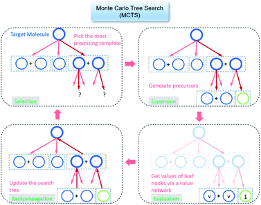 | ||
| Fig. 1 The process of Monte Carlo Tree Search in synthesis planning. Following the notations of MDP, a molecule (or state) is denoted as s, and a template (or retrosynthetic disconnection action) is denoted as a. In the selection phase, starting from the target molecule, the most “promising” template is recursively chosen by selecting the template with the highest upper confidence bound (UCB(s,a)) value until a leaf node is reached. A policy network is used to narrow down the search beam in each template selection step. In the expansion phase, the leaf node is expanded by applying the selected template. New leaf nodes (precursors) that are not visited by the tree expander before are generated. Once the new leaf nodes are encountered, in the evaluation step, a value network is used to evaluate the values of the leaf nodes (if the node is buyable, the value is set to 1). Then in the backpropagation step, upward along the tree, the visit count N(s,a) of each compound-template (s,a) pairs, or edges, are updated. The Q(s,a) value (see Table 1) is recalculated as well and used to recompute UCB(s,a) values in the next selection step. With the updated values, the tree expander goes back to the selection phase, starting selecting the most promising template for the target molecule (root node) again. Here circles denote compounds. (Blue) not commercially available; (Green) commercially available. | ||
 denotes the summation of N(s,b) over all allowable templates b available for state s. v(s) is the value of s and the output of the value network. s,a → s′ indicates that s′ is eventually reached after taking action a from position s
In addition, instead of using a Monte Carlo roll-out1,28,29 as the look-ahead mechanism in the “Evaluation” step, we use a value network to generate the value of a compound, similar to Alpha Go by Silver et al.22 and envisioned by Segler et al.1 If the compound is in our buyable catalog, the value will be set to 1 and overwrite the value given by the value network. The value network is trained through RL self-play. The self-play process (bootstrapping) and the definition of values are discussed in the following part. The value network trained in this way is therefore dependent on the buyable catalogue used.
As shown in Table 1, in total, we study 6 MCTS variants: modified UCT with dynamic c and value network (mUCT-dc-V), original UCT with value network (UCT-V), modified UCT without dynamic c with value network (mUCT-V), PUCT22,31 MCTS with value network (PUCT-V, is very similar to the MCTS used by Segler et al.1), PUCT MCTS without value network (PUCT-bootstrapping), modified UCT with dynamic c but without value network (mUCT-dc-bootstrapping).
Training the value network using RL for efficient synthesis planning
The MCTS process requires a reliable policy network and value network. The training process of the policy network in this work is described in the Methods, and it is very similar to the process used by Segler et al.1,23,24 The training of the value network is one of the main points of this work. First of all, the value of a compound should reflect the “easiness” of synthesis based on the buyable catalog. Therefore defining the “easiness” and getting enough data for this standard is critical. At the same time, modifications to the MCTS algorithm are required to tolerate some inherent issue of the policy and value network and guarantee that synthesis planning is still successful even with a non-ideal policy/value network. To tackle these two challenges, we develop reinforcement learning (RL) and a modified UCT algorithm with dynamic c tuning for the first time.RL and bootstrapping
In order to maximize the success rate of the search, we consider the value of a state (or compound) as follows,40 We only consider the deterministic case where T(s,a,s′) = 1, if s′ is the result of retrosynthetic disconnection action a (or template) taken by compound s, otherwise T(s,a,s′) = 0; and we set R(s,a,s′)to 0 for all reactions. If s′ is buyable, v*(s′) = 1. Therefore
Here s′ is the next state of s so that T(s,a,s′) = 1. A(s) is the action space which defines all the allowable retrosynthetic disconnection actions for s. Note that the definition of v*(s) is recursive and depending on ergodic search in the action space, which is not possible. It is prohibitive to obtain the analytical solution of the exact value of v*(s). Instead, we can empirically approximate v*(s) by running MCTS on molecules randomly sampled from the chemical space. The resulting approximate of v*(s) through MCTS sampling is z(s), and the output of the value network trained using z(s) is defined as vθ(s), so that vθ(s) ≈ z(s) ≈ v*(s).
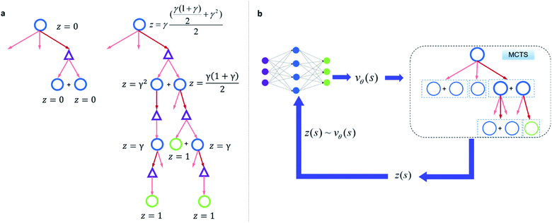
Since one compound s can be split into multiple compounds, defining z(s) is complex. In order to bootstrap the process, we define the z(s) value for each compound in the tree as shown in Fig. 2a. The z(s) is defined similar to the Bellman equation of v*(s)40 with a discount factor of γ. For a reaction ((s,a) pair) in the tree, if all of its child compounds (s′) have a non-zero z value, then a Z(s,a) value for the reaction is defined as the average z value of its children, and the z value of the parent compound, s, is defined as the maximum Z(s,a) value multiplied by γ among all actions available to s in the tree.
By initialization, the z values for the compounds are zero. Along the tree search process, the encountered compounds in the buyable catalog will be assigned a z(s) of 1, as shown in Fig. 2a. In the bootstrapping phase, no value network is used. The Q(s,a) value, which is important in UCB equations, is calculated using z(s) values in the bootstrapping phase as shown in Table 1. Therefore in this process, a strong favor will be given to those actions which can lead to buyable products fast.
The z(s) values are obtained retrospectively, i.e., they can only be calculated after running the MCTS. In order to guide the retrosynthesis, we need to evaluate the value prospectively, so we train a value function vθ(s) that only takes molecular structure as an input to predict z(s) (Fig. 2b). The value network can be further updated with more z(s) data accumulate during the training of the RL algorithm. In this work, we will discuss the value network obtained by the Round 1 RL (trained with z(s) values generated from bootstrapping MCTS) and the Round 2 RL (trained with z(s) values generated from MCTS with the Round 1 RL value network). The bootstrapping MCTS variant used here is the mUCT-dc-bootstrapping method. The details of the RL value network training can be found in the Methods section.
Performance of the novel MCTS variant and RL value network in finding successful synthetic routes
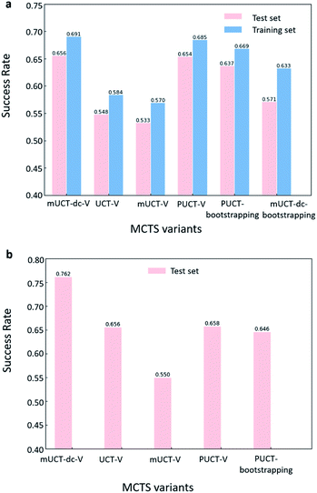
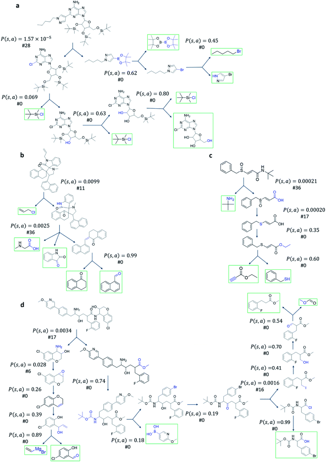
The performance of different MCTS variants is shown in Fig. 3. We conduct two types of experiments: tree expansion with a fixed expansion time of 30 s (Fig. 3a); and tree expansion with a fixed root visit count (Fig. 3b), which is independent of computers used and thus more reproducible.Among all the MCTS variants, for our test set of 1000 compounds, the mUCT-dc-V and PUCT-V algorithms outperform the other variants with a fixed expansion time of 30 s (Fig. 3a). Especially when compared to the original UCT method (UCT-V), the mUCT-dc-V outperforms by 19.7% with the same value network and same initialization of the c value. This is a result of the active exploration promoted by the dynamic c tuning. Without the dynamic c, the performance of the modified UCT without dynamic c (mUCT-V) and the original UCT method (UCT-V) are very close. In addition, mUCT-dc-V is able to find synthesis pathways in 30 s for many target compounds that cannot be solved by PUCT-V method, providing a new effective approach to finding synthetic pathways connecting targets to buyable chemicals (cf.Fig. 4).
Fig. 4 shows the probability P(s,a) of each step (s,a) given by the policy network together with the ranking of the template among the top 50 templates suggested by the policy network. The success of the mUCT-dc-V method is attributed to templates with small P(s,a) and low ranking can still be effectively explored due to the dynamic tuning of the exploration coefficient c in the UCB equation. On the contrary, PUCT-V tree expander is trapped by the high ranking templates that eventually are insufficient in forming a valid synthetic route, as a result of a more greedy strategy in the definition of its UCB equation.
Traditionally, since PUCT utilizes the information of the prior probabilities of different templates explicitly, it does not need to compute the logarithmic function (Table 1) and will search more quickly. As a result, the PUCT algorithm outperforms the original UCT method. However, with the dynamic c to promote active exploration, the mUCT-dc-V method even outperforms the PUCT algorithm in both test sets and training sets. In addition, since the policy network trained on the Reaxys database focuses only on single step transformations and does not necessarily reflect the best prior probability P(s,a) that helps maximize the success rate of multi-step retrosynthesis search, it may mislead the PUCT algorithm. In contrast, UCT type MCTS variants do not explicitly include the P(s,a) into the equation for UCB (Table 1). Instead, they only use the results of the policy network to shrink the width of the searching. Therefore modified UCT with dynamic c trick (mUCT-dc-V) is more robust against the imperfect policy network quality and the forced exploration guarantees broader selection of templates and more various synthesis routes, which will lead to greener pathways as we will show in the following parts.
When the termination criteria of tree expansion is switched to a fixed root visit count, the advantage of mUCT-dc-V algorithm is even more obvious (Fig. 3(b)). The power of dynamic c makes the modified UCT method outperform the PUCT-V method by ∼16%. Since the UCT method requires the computation of the logarithmic function and forces exploration of low ranked templates, UCT searches much slower than the PUCT method. With 30 s as time limit, UCT actually visits the root much less than the PUCT method. However with the dynamic c trick, our novel UCT is able to search more efficiently and have a slightly higher success rate compared to PUCT. When both methods are given the same root visit count limit, the mUCT-dc-V method largely outperforms the PUCT method due to the more efficient searching.
The value network used in Fig. 3 is the value network from Round 1 RL. The results of Round 2 RL value network can be found in Table S1 in the ESI† and are not significantly different from the results of Round 1 RL value network. The c value is 0.1 for UCT type MCTS variants, and is set to 1 for PUCT type of MCTS variants. The effect of different c values is studied in Table 2, and it does not significantly affect the performance. Here the values for buyable compounds are set to be 1 during the tree search regardless of the prediction of the value network. The results of the tree expansion without the prior knowledge of buyable compounds during value setting is shown in Fig. S1 and Table S2 in the ESI.† In general, the performance is much worse than the case in Fig. 3, implying that the MCTS tree expander favors pathways with strong incentive such as high weight for buyable compounds.
Incorporating solvent greenness into synthesis planning
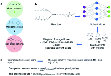
With a high success rate supported by the mUCT-dc-V method, MCTS is also able to steer the synthesis planning towards greener processing routes. Here, we focus on using MCTS, RL and mUCT-dc-V to find synthesis routes with fewer steps and greener solvents. Although we focus on the solvent greenness and the length of the synthetic routes, the same method can be extended to other green chemistry considerations, such as mild reaction temperatures and economical catalysts.34We assign different scores to different solvents in our solvent library based on biosafety and flammability as suggested by Byrne et al.41 “Green” solvents, such as ethanol and water, are assigned the score of 1. “Mediocre” solvents, such as methyl isobutyl ketone (MIBK) and toluene, are given the score of 0. “Non-green” solvents, such as tetrachloromethane and 1,2-dimethoxyethane, are allotted a negative score of −1 (see Fig. 5a). Gao et al.34 proposed a neural network model that can predict suitable solvents with a probability distribution when given a target reaction. Based on this result, we define the reaction solvent score as the weighted average of the suggested solvents by the solvent model (Fig. 5b). The solvent model suggests a list of solvents for the desired reaction with different probabilities. This probability-weighted greenness is akin to Li and Eastgate's work for incorporating ligand information into process mass intensity (PMI).42 With the idea of reaction solvent score, a compound solvent score can be defined. We first convert the reaction solvent score (RSS ∈ [−1,1]) to reaction solvent penalty (RSP ∈ [−1,−0.1]) (Fig. 5c). The idea of reaction solvent penalty is that any additional reaction is “bad” for the goal of finding shortest possible synthetic routes, therefore all reactions should be penalized. Yet reactions using “green” solvents should be less penalized than the non-green reactions. Therefore, the reactions with RSS of 1 receives only a small penalty of −0.1, while the reactions using very toxic or flammable solvents (RSS = −1) are given the most negative penalty −1. Then we are able to define compound solvent score (CSS) as
The optimization problem to maximize the route greenness boils down to the problem of finding the greenest valid route argmaxpath(ΣR in Path (R penalty in the path)) for the root compound. We use the CSS of the root compound as the greenness of the synthetic route in this work. Moreover, the overall goal is to optimize the compound solvent scores of the root compounds (or route greenness) by developing efficient MCTS tree expanders.
Performance of finding routes leading to high compound solvent scores
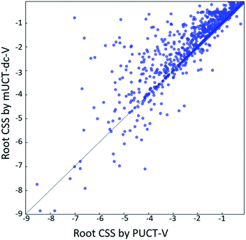
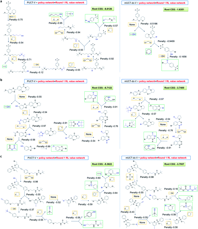
The modified UCT method with dynamic c tuning(mUCT-dc-V) significantly outperforms the PUCT MCTS (PUCT-V) method in terms of finding greener synthesis routes, when using the same value network (Round 1 RL value network) and policy network. We run the MCTS tree expansion on 2000 randomly selected testing compounds for 30 s. Among the root compounds that are solvable for both MCTS variants, 74% of them demonstrated CSS(mUCT-dc-V) ≥ CSS(PUCT-V) in 30 s MCTS tree expansion, and 71.4% of the compounds are improved by the mUCT-dc-V method (Fig. 6). Fig. 7 shows examples of the compounds that are solvable to both MCTS variants but show quite different solvent greenness in resulting synthetic routes. The key is that PUCT algorithm always tends to find long synthetic pathways without fully exploring the template space.The reason for mUCT-dc-V generating greener synthetic routes lies in the intrinsic difference of the PUCT MCTS and the modified UCT with dynamic c MCTS. In the UCB equation of PUCT-V (Table 1), the output of the policy network P(s,a) is explicitly used in the exploration term to steer the tree expander to select templates with higher prior probability. However, the policy network trained on the Reaxys database does not necessarily reflect the true value of the prior probability, although the relative ranking given by the policy network is meaningful. Therefore, with an inaccurate prior probability value, the PUCT MCTS can be misled by the policy network. On the contrary, the forced exploration by the dynamic c tuning in the modified UCT MCTS provides a broader vision to explore templates that are underestimated by the policy network, since the value of the prior probability is not used explicitly in the UCB equation here but only the ranking is used. In addition, since P(s,a) for many low ranked templates is extremely small as a result of the imperfect policy network, the templates are not effectively explored by the PUCT MCTS. As a consequence, the PUCT MCTS tree expander will prefer to exploring edges that policy network prefers instead of exploring templates that might be ranked lower but can eventually yield shorter routes.
We also trained a value network using the CSS values generated from MCTS experiments. The route greenness is worse than the value networks only considering synthetic “easiness” (i.e. Round 1 RL value network). The main reason is that the CSS value based value network sacrifices the success rate of the synthesis planning. Consequently with deficient routes to choose from, the CSS value network is worse at finding green pathways. The loss–iteration curve of the CSS value network can be found in Fig. S2.† The comparison of the performances of CSS value network and the Round 1 RL value network can be found in Table S3.†
We have also compared the performance of PUCT-bootstrapping method with the mUCT-dc-V with Round 1 RL value network. The novel UCT method again defeats the PUCT-bootstrapping algorithm in terms of the solvent greenness of the generated synthetic routes. The performance can be found in Table S4 in the SI.†
Conclusions
We developed a new MCTS variant, modified UCT with dynamic c tuning, leading to a much improved success rate in finding valid synthesis pathways compared with the original UCT method by using the new method with a RL trained value network as a look-ahead mechanism. The success rate of the new MCTS variant is comparable to the Alpha Go-like PUCT MCTS algorithm. With a fixed root visit count, the MCTS variant significantly outperforms the PUCT MCTS, meaning its search is more visit-count efficient. Furthermore, when considering the route greenness, our MCTS variant is able to beat the PUCT algorithm with 71.4% pathways improved. The new MCTS is successful in generating much shorter pathways since it is not misled by the imperfect policy network thanks to the forced exploration promoted by the dynamic c tuning. Our work paves the way towards design of shorter synthesis pathways for organic molecules with greener processes. Furthermore, our modified algorithm allows the user to incorporate additional reaction-level of pathway-level penalties to bias exploration besides the considerations in green chemistry.Methods
Details of synthesis planning as a tree search problem
Starting from the target molecule, a deep neural network (policy network) outputs a probability distribution22p(a|s) = P(s,a) over the allowed deconstruction actions a ∈ A(s) (the reaction templates). The policy network is used to rank the possibilities associated with different templates. We use the top 50 templates suggested by the policy network in the experiments of this article. In the initial round, the template with the highest ranking is visited first. In the regular round, the upper confidence bound (UCB) of each edge (state-action pair, (s,a), i.e. the compound-template pair) of the tree is calculated using the UCB equations shown in Table 1. In the UCT type MCTS (the first three rows of Table 1), the UCB equations are not explicitly related to the output of the policy network, except that the template is ranked by the policy network, and the templates are visited in the ranked order. However, in the Alpha Go-like PUCT MCTS (PUCT in Table 1), the P(s,a) is explicitly incorporated in the exploration term, steering a stronger favor towards exploiting highly probable actions/templates.The most promising template selected for each compound s is the template with the highest UCB(s,a) value. This template selection process takes place recursively in the tree until a leaf node (nodes without a child along the edge of the most promising template) is encountered. The tree expander will expand the leaf node by applying the selected template to it. In this way, new leaf nodes (new precursors) are added to the tree. Once the new leaf nodes are generated, a second neural network, value network, is used to evaluate the novel compounds. We check the commercial availability of the leaf nodes and once the leaf nodes are found to be in our catalogue of purchasable compounds, the value of this compound is set to 1 (overwriting the value given by the value network) and this node will not undergo an expansion process any more. The tree expansion settings are: top 50 templates given by policy network are considered, maximum depth is 10, and minimum plausibility is 0.75. The minimum plausibility is the output of a fast filter based on a model predicting the likelihood of a reaction being plausible.17
Once we get the values of the leaf compounds, a backpropagation process takes place. In the backpropagation step, visit counts (N(s,a)) and template Q value (Q(s,a)) are updated for all the (s,a) pairs (compound-template pairs) upward on the tree as shown in Fig. 1. The equation to calculate Q(s,a) is shown in Table 1. In practice, we also update z(s) value (which is explained in the bootstrapping part) along the MCTS process in the bootstrapping phase. After the backpropagation, the tree expander select the most promising template with the highest UCB(s,a) from the target molecule (root node) again with the updated template visit count (N(s,a)) and template Q value (Q(s,a)).
The modified UCT with a dynamic c tuning
The UCB equation of the original UCT28,29 MCTS (Table 1) is usually called the UCB1 (ref. 30 and 31) equation. In this work, a dynamic c tuning was used on the basis of the modified UCB equation for UCT algorithm28,29 (or modified UCB1 (ref. 30) equation) (Table 1). The analysis of the modified UCB1 equation can be found in the ESI.† The dynamic c trick is to: (1) enhance the sampling rate and dynamically tune the exploration rate, (2) to balance the imperfect policy network.A key issue of the modified UCB1(see the ESI†) and the original UCB1 in MCTS is that the tree expander may tend to visit the known best action too many times and it does not sample other options enough, when the parameter c is not appropriate. Additionally, when the value network cannot evaluate the states perfectly, it is important to explore the actions efficiently in a dynamic way. Therefore, we proposed the dynamic c trick to solve these challenges, and as shown in the main text, it significantly improves performance of the MCTS algorithm.
First of all, we have a policy network that ranks the probability to apply each template (or action). Therefore we always start from the highest ranked template and then visit the second ranked and so on. The event we want to investigate is the case when the tree expander switches from the highest ranked template to the second highest ranked template when using modified UCB1 equation.
Suppose that in the last round, the expanded template (action a) has the  and the next unexpanded template has a
  the unexpended template will not be visited in the current round unless
Specifically, if the switching is between the highest ranked template and the second highest ranked template, ∑bN(s,b) = N(s,a), since only the highest ranked template a is visited. Therefore the minimum N(s,a) required for the highest ranked template a can be solved from
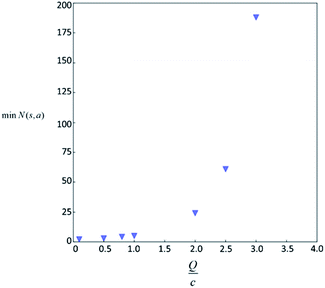
Therefore the minimum required visit time N(s,a) depends on the ratio of Q(s,a) and c.The solution of this inequality vs. the value of Q/c is shown in Fig. 8 and Table 3. As Q/c value increases, the minimum required N(s,a) increases very rapidly. Therefore if we don't choose c carefully, the tree expander will be searching the highest ranked template almost forever. If the highest ranked template cannot lead to a buyable pathway, the tree expander is “trapped” in this suboptimal branch. The phenomena shown in Fig. 8 and Table 3 also comport with the idea that c is promoting “exploration” in the sense that the extent to which c is promoting exploration depends on its relative value to Q.
| Q/c value | min N(s,a) |
|---|---|
| 4 | 3879 |
| 5 | 281326 |
| 9 | 3.88 × 10¹⁷ |
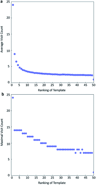
In practice, here we choose Q/c = 2 as the standard. Therefore the first template switch will happen when the first template has been visited for 24 times. If we set  for all visited Q(s,b) values and we assume random variables Q(s,b) ∈ (0,1) (this is the requirement of Chernoff–Hoeffding bound30 and is the actual case in this paper) are not changing with tree expansion, the average and maximal visit count for each template before all templates are visited can be calculated as shown in Fig. 9 (a and b) using 104 random simulations. In fact, this trick allows visiting all the templates with decaying visit times according to their ranking given by the policy network.
One issue for the aforementioned strategy is, the Q(s,b) values are actually changing as the tree expands. Therefore we propose a method to tune the c on the go. The idea is shown in Fig. 10. The value of c is tuned as current observed max Q/2 as the tree expands. The benefit of this promoted exploration of low ranked templates can be seen in Fig. 4, where low ranked templates lead to successful synthetic routes while PUCT-V method is trapped in the high ranked templates which eventually are insufficient in forming a valid synthetic route.
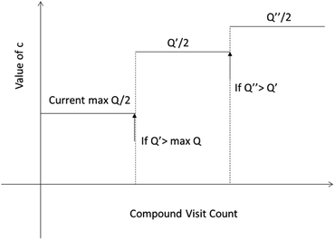 | ||
| Fig. 10 The dynamic method to decide the value of c. We define c as half of the current max Q(s,b) value during the tree expansion process during which the visit count of the compound s increases. | ||
The training of value networks with round 1 RL
The data z(s) values are collected from 40 s tree expansion (mUCT-dc-bootstrapping) for 112![[thin space (1/6-em)]](https://www.rsc.org/images/entities/char_2009.gif) 000 product molecules randomly selected from the Reaxys database.
000 product molecules randomly selected from the Reaxys database.
The tree expansion generates z(s) values for all compounds generated in the 112![[thin space (1/6-em)]](https://www.rsc.org/images/entities/char_2009.gif) 000 trees in the way shown in Fig. 2a. In the Round 1 RL, γ = 0.9. Also, since for the same compound s, the z(s) value can depend on the timing it appears in the trees, we choose z(s) as the maxz(s)∀ trees where compound s appears. The data is then scaled to [0.2, 1] based on the equation:
000 trees in the way shown in Fig. 2a. In the Round 1 RL, γ = 0.9. Also, since for the same compound s, the z(s) value can depend on the timing it appears in the trees, we choose z(s) as the maxz(s)∀ trees where compound s appears. The data is then scaled to [0.2, 1] based on the equation:
![[thin space (1/6-em)]](https://www.rsc.org/images/entities/char_2009.gif) 000 trees, there are 695
000 trees, there are 695![[thin space (1/6-em)]](https://www.rsc.org/images/entities/char_2009.gif) 574 z′(s) values generated. We then split the data set with 8
574 z′(s) values generated. We then split the data set with 8![[thin space (1/6-em)]](https://www.rsc.org/images/entities/char_2009.gif) :
:![[thin space (1/6-em)]](https://www.rsc.org/images/entities/char_2009.gif) 2 ratio randomly to formulate the training set and test set for the value network.
2 ratio randomly to formulate the training set and test set for the value network.
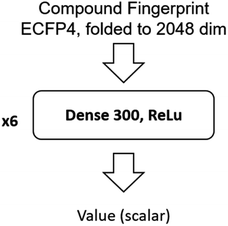
The input of the value network is the Morgan fingerprint of the compound converted by RDKit. The architecture of the value network is shown in Fig. 11.
The loss–iteration curve can be found in Fig. S2.† The mean squared error (MSE) of the test set is also tested. MSE of round 1 RL value network on the test set is ∼0.031 and MSE of round 2 RL value network on the test set is ∼0.02. Considering the MSE of the value network in Deep Mind's Alpha Go algorithm22 is ∼0.226 for training set and ∼0.234 for test set, our value networks' MSE's are much lower, when the value v(s) is bounded within (0,1] for both cases, which is a requirement of Chernoff-Hoeffding bound.30
The buyable compounds
Buyable compounds are a collection of ∼107![[thin space (1/6-em)]](https://www.rsc.org/images/entities/char_2009.gif) 000 compounds with a list price of under $100 per g from SigmaAldrich and eMolecules with salts removed.17 The lookup function is part of the open source ASKCOS website.43
000 compounds with a list price of under $100 per g from SigmaAldrich and eMolecules with salts removed.17 The lookup function is part of the open source ASKCOS website.43
The training of value networks with round 2 RL
In the Round 2 RL training of value networks, the data z(s) values are generated from 40 s tree expansion using the mUCT-dc-V algorithm for 62![[thin space (1/6-em)]](https://www.rsc.org/images/entities/char_2009.gif) 000 compounds among the 112
000 compounds among the 112![[thin space (1/6-em)]](https://www.rsc.org/images/entities/char_2009.gif) 000 compounds used in Round 1 RL value network training, in order to save workload. Here the value network used for MCTS tree expansion is the value network trained in round 1 RL. The γ here is set to be 0.7 to enhance the differentiation of synthesis “easiness”. We again choose z(s) as the maxz(s) ∀ trees where compound s appears. Then after adding z(s) = 1for the buyable compounds encountered in the 62
000 compounds used in Round 1 RL value network training, in order to save workload. Here the value network used for MCTS tree expansion is the value network trained in round 1 RL. The γ here is set to be 0.7 to enhance the differentiation of synthesis “easiness”. We again choose z(s) as the maxz(s) ∀ trees where compound s appears. Then after adding z(s) = 1for the buyable compounds encountered in the 62![[thin space (1/6-em)]](https://www.rsc.org/images/entities/char_2009.gif) 000 trees, we get 321
000 trees, we get 321![[thin space (1/6-em)]](https://www.rsc.org/images/entities/char_2009.gif) 395 z(s) values. We split them with 8
395 z(s) values. We split them with 8![[thin space (1/6-em)]](https://www.rsc.org/images/entities/char_2009.gif) :
:![[thin space (1/6-em)]](https://www.rsc.org/images/entities/char_2009.gif) 2 ratio and get a training set of 257
2 ratio and get a training set of 257![[thin space (1/6-em)]](https://www.rsc.org/images/entities/char_2009.gif) 116 compounds and a test set of 64
116 compounds and a test set of 64![[thin space (1/6-em)]](https://www.rsc.org/images/entities/char_2009.gif) 279 compounds.
279 compounds.
The training of value networks based on compound solvent scores
In the Round 2 RL, we also collected the CSS values generated from the tree expansion of the 62![[thin space (1/6-em)]](https://www.rsc.org/images/entities/char_2009.gif) 000 compounds. In total, we collected CSS(s) value for 282
000 compounds. In total, we collected CSS(s) value for 282![[thin space (1/6-em)]](https://www.rsc.org/images/entities/char_2009.gif) 398 compounds successfully solved in the tree expansion. Then we split them with 8
398 compounds successfully solved in the tree expansion. Then we split them with 8![[thin space (1/6-em)]](https://www.rsc.org/images/entities/char_2009.gif) :
:![[thin space (1/6-em)]](https://www.rsc.org/images/entities/char_2009.gif) 2 ratio and get a training set of 225
2 ratio and get a training set of 225![[thin space (1/6-em)]](https://www.rsc.org/images/entities/char_2009.gif) 918 compounds and a test set of 56
918 compounds and a test set of 56![[thin space (1/6-em)]](https://www.rsc.org/images/entities/char_2009.gif) 480 compounds.
480 compounds.
The training of the policy network and the extraction of templates
The training of the policy network is similar to the work by Segler et al.1,23. With an input of the Morgan fingerprint, the policy network gives the probability distribution p(a|s) = P(s,a) over the allowed actions (templates) a ∈ A(s). The policy network is trained on 5.4 million reaction examples from Reaxys. The training and validation details and the model architecture can be found on Github.35 The extraction of templates is described in our previous work.44RSS calculation
We used the same reaction condition prediction model as described in Gao et al.34 The model predicts catalysts, solvents and reagents in a sequential manner. Since we only consider solvent greenness, we only use part of the model. Given a reaction, the model first predicts a catalyst, and combine the catalyst and reaction information to predict a solvent. We took the softmax scores for the top 3 solvent predictions and calculated a weighted sum as the RSS, as follows:where nn(soli) is the softmax score given by the neural network model for solvent prediction. greenness(soli)is the greenness score of the solvents, which is defined in the way shown in Fig. 5. The definition of green, mediocre and non-green solvents is as reported by Byrne et al.41
Training set and test set of the MCTS success rate experiments and greenness tests
The training set in Fig. 3 is the training set of the 112![[thin space (1/6-em)]](https://www.rsc.org/images/entities/char_2009.gif) 000 compounds used in the bootstrapping phase. We randomly choose 1000 compounds from the training set of the value network training for test purpose of MCTS success rate experiment. The 1000 compounds from the training set are the same for all MCTS variants in Fig. 3.
000 compounds used in the bootstrapping phase. We randomly choose 1000 compounds from the training set of the value network training for test purpose of MCTS success rate experiment. The 1000 compounds from the training set are the same for all MCTS variants in Fig. 3.
The test set for the MCTS experiments in Fig. 3 are different from the test set of the value network validation. We choose the compounds in the Reaxys data base that are not in the training sets used in training the value networks, and are not in the “training set” in MCTS success rate experiments. There are in total 1![[thin space (1/6-em)]](https://www.rsc.org/images/entities/char_2009.gif) 673
673![[thin space (1/6-em)]](https://www.rsc.org/images/entities/char_2009.gif) 879 compounds in Reaxys that are not seen in the previous value network training process, and we use these compounds as the test set for MCTS success rate testing. In the MCTS success rate experiments shown in Fig. 3, we choose 1000 compounds from the test set randomly. The 1000 tested compounds from the test set are the same for all MCTS variants in Fig. 3.
879 compounds in Reaxys that are not seen in the previous value network training process, and we use these compounds as the test set for MCTS success rate testing. In the MCTS success rate experiments shown in Fig. 3, we choose 1000 compounds from the test set randomly. The 1000 tested compounds from the test set are the same for all MCTS variants in Fig. 3.
The test set of the greenness tests in Fig. 6 is randomly selected 2000 compounds from the test set, and Tables S3 and S4† is randomly selected 500 compounds from the 1000 tested compounds used in the success rate experiments.
Conflicts of interest
There are no conflicts to declare.Acknowledgements
This work was supported by Machine Learning for Pharmaceutical Discovery and Synthesis Consortium. X. W. acknowledge the support from the Ohio State University. The authors sincerely thank Mr Clemens Isert from ETH Zürich for the inspiring discussion about reaction solvent penalties.Notes and references
- M. H. S. Segler, M. Preuss and M. P. Waller, Nature, 2018, 555, 604–610 Search PubMed.
- J. L. Baylon, N. A. Cilfone, J. R. Gulcher and T. W. Chittenden, J. Chem. Inf. Model., 2019, 59, 673–688 Search PubMed.
- J. S. Schreck, C. W. Coley and K. J. M. Bishop, ACS Cent. Sci., 2019, 5, 970–981 Search PubMed.
- A. Cook, A. P. Johnson, J. Law, M. Mirzazadeh, O. Ravitz and A. Simon, WIREs Comput. Mol. Sci., 2012, 2, 79–107 Search PubMed.
- S. Szymkuć, E. P. Gajewska, T. Klucznik, K. Molga, P. Dittwald, M. Startek, M. Bajczyk and B. A. Grzybowski, Angew. Chem., Int. Ed., 2016, 55, 5904–5937 Search PubMed.
- E. J. Corey and W. T. Wipke, Science, 1969, 166, 178 Search PubMed.
- E. J. Corey and W. L. Jorgensen, J. Am. Chem. Soc., 1976, 98, 189–203 Search PubMed.
- C. W. Coley, W. H. Green and K. F. Jensen, Acc. Chem. Res., 2018, 51, 1281–1289 Search PubMed.
- T. Badowski, K. Molga and B. A. Grzybowski, Chem. Sci., 2019, 10, 4640–4651 Search PubMed.
- C. A. Nicolaou, I. A. Watson, M. LeMasters, T. Masquelin and J. Wang, J. Chem. Inf. Model., 2020, 60(6), 2728–2738 Search PubMed.
- G. É. Vléduts, Inf. Storage Retr., 1963, 1, 117–146 Search PubMed.
- S. Soh, Y. Wei, B. Kowalczyk, C. M. Gothard, B. Baytekin, N. Gothard and B. A. Grzybowski, Chem. Sci., 2012, 3, 1497–1502 Search PubMed.
- B. A. Grzybowski, K. J. M. Bishop, B. Kowalczyk and C. E. Wilmer, Nat. Chem., 2009, 1, 31–36 Search PubMed.
- K. J. M. Bishop, R. Klajn and B. A. Grzybowski, Angew. Chem., Int. Ed., 2006, 45, 5348–5354 Search PubMed.
- M. Fialkowski, K. J. M. Bishop, V. A. Chubukov, C. J. Campbell and B. A. Grzybowski, Angew. Chem., Int. Ed., 2005, 44, 7263–7269 Search PubMed.
- K. Molga, P. Dittwald and B. A. Grzybowski, Chem, 2019, 5, 460–473 Search PubMed.
- C. W. Coley, D. A. Thomas, J. A. M. Lummiss, J. N. Jaworski, C. P. Breen, V. Schultz, T. Hart, J. S. Fishman, L. Rogers, H. Gao, R. W. Hicklin, P. P. Plehiers, J. Byington, J. S. Piotti, W. H. Green, A. J. Hart, T. F. Jamison and K. F. Jensen, Science, 2019, 365, eaax1566 Search PubMed.
- D. J. C. Constable, P. J. Dunn, J. D. Hayler, G. R. Humphrey, J. J. L. Leazer, R. J. Linderman, K. Lorenz, J. Manley, B. A. Pearlman, A. Wells, A. Zaks and T. Y. Zhang, Green Chem., 2007, 9, 411–420 Search PubMed.
- S. G. Koenig, D. K. Leahy and A. S. Wells, Org. Process Res. Dev., 2018, 22, 1344–1359 Search PubMed.
- P. Schwaller, T. Laino, T. Gaudin, P. Bolgar, C. A. Hunter, C. Bekas and A. A. Lee, ACS Cent. Sci., 2019, 5, 1572–1583 Search PubMed.
- D. Silver, J. Schrittwieser, K. Simonyan, I. Antonoglou, A. Huang, A. Guez, T. Hubert, L. Baker, M. Lai and A. Bolton, Nature, 2017, 550, 354–359 Search PubMed.
- D. Silver, A. Huang, C. J. Maddison, A. Guez, L. Sifre, G. van den Driessche, J. Schrittwieser, I. Antonoglou, V. Panneershelvam, M. Lanctot, S. Dieleman, D. Grewe, J. Nham, N. Kalchbrenner, I. Sutskever, T. Lillicrap, M. Leach, K. Kavukcuoglu, T. Graepel and D. Hassabis, Nature, 2016, 529, 484–489 Search PubMed.
- M. H. S. Segler and M. P. Waller, Chem.–Eur. J., 2017, 23, 5966–5971 Search PubMed.
- M. H. Segler, arXiv preprint arXiv:1912.13007, 2019.
- A. Kishimoto, B. Buesser, B. Chen and A. Botea, Adv. Neural. Inf. Process. Syst., 2019, 7224–7234 Search PubMed.
- B. Chen, C. Li, H. Dai and L. Song, arXiv preprint arXiv:2006.15820, 2020.
- J. S. Schreck, https://github.com/jsschreck/retroRL.
- S. James, G. Konidaris and B. Rosman, An Analysis of Monte Carlo Tree Search, 2017 Search PubMed.
- L. Kocsis and C. Szepesvári, European conference on machine learning, 2006, pp. 282–293 Search PubMed.
- P. Auer, N. Cesa-Bianchi and P. Fischer, Mach. Learn., 2002, 47, 235–256 Search PubMed.
- C. D. Rosin, Ann. Math. Artif. Intell., 2011, 61, 203–230 Search PubMed.
- H. Struebing, Z. Ganase, P. G. Karamertzanis, E. Siougkrou, P. Haycock, P. M. Piccione, A. Armstrong, A. Galindo and C. S. Adjiman, Nat. Chem., 2013, 5, 952–957 Search PubMed.
- G. Marcou, J. Aires de Sousa, D. A. R. S. Latino, A. de Luca, D. Horvath, V. Rietsch and A. Varnek, J. Chem. Inf. Model., 2015, 55, 239–250 Search PubMed.
- H. Gao, T. J. Struble, C. W. Coley, Y. Wang, W. H. Green and K. F. Jensen, ACS Cent. Sci., 2018, 4, 1465–1476 Search PubMed.
- C. W. Coley, https://github.com/connorcoley/retrotemp/tree/master/retrotemp.
- C. W. Coley, L. Rogers, W. H. Green and K. F. Jensen, ACS Cent. Sci., 2017, 3, 1237–1245 Search PubMed.
- K. Lin, Y. Xu, J. Pei and L. Lai, Chem. Sci., 2020, 11, 3355–3364 Search PubMed.
- B. Liu, B. Ramsundar, P. Kawthekar, J. Shi, J. Gomes, Q. Luu Nguyen, S. Ho, J. Sloane, P. Wender and V. Pande, ACS Cent. Sci., 2017, 3, 1103–1113 Search PubMed.
- P. Karpov, G. Godin and I. V. Tetko, International Conference on Artificial Neural Networks, 2019, pp. 817–830 Search PubMed.
- R. S. Sutton and A. G. Barto, Reinforcement learning: An introduction, MIT press, 2018 Search PubMed.
- F. P. Byrne, S. Jin, G. Paggiola, T. H. M. Petchey, J. H. Clark, T. J. Farmer, A. J. Hunt, C. Robert McElroy and J. Sherwood, Sustainable Chem. Processes, 2016, 4, 7 Search PubMed.
- J. Li and M. D. Eastgate, React. Chem. Eng., 2019, 4, 1595–1607 Search PubMed.
- C. W. Coley, http://askcos.mit.edu/#.
- C. W. Coley, W. H. Green and K. F. Jensen, J. Chem. Inf. Model., 2019, 59, 2529–2537 Search PubMed.
Footnote |
| † Electronic supplementary information (ESI) available. See DOI: 10.1039/d0sc04184j |
| This journal is © The Royal Society of Chemistry 2020 |


