Discrete Helmholtz model: a single layer of correlated counter-ions. Metal oxides and silica interfaces, ion-exchange and biological membranes

Abstract

The mechanism by which interfaces in solution can be polarised depends on the nature of the charge carriers. In the case of a conductor, the charge carriers are electrons and the polarisation is homogeneous in the plane of the electrode. In the case of an insulator covered by ionic moieties, the polarisation is inhomogeneous and discrete in the plane of the interface. Despite these fundamental differences, these systems are usually treated in the same theoretical framework that relies on the Poisson–Boltzmann equation for the solution side. In this perspective, we show that interfaces polarised by discrete charge distributions are rather ubiquitous and that their associated potential drop significantly differs from those of conductor–electrolyte interfaces. We show that these configurations, spanning liquid–liquid interfaces, charged silica–water interfaces, metal oxide interfaces, supercapacitors, ion-exchange membranes and even biological membranes can be uniformly treated under a common “Discrete Helmholtz” model where the discrete charges are compensated by a single layer of correlated counter-ions, thereby generating a sharp potential drop at the interface.

---

Introduction

When describing electrolytes at a polarised metallic electrode, the structure of the electrode itself is often omitted. Thus, classical models assume that ions in solution respond to the presence of an electric potential originating from a homogeneous electrode that is only considered as a mathematical constraint on the boundary conditions of a differential equation. Nevertheless, this assumption allowed for the development of models that gave significant insight on the behaviour of electrolytes close to a polarised interface, but established the view that most of the physics take place on the solution side of the interface. The first of these models was that proposed by Helmholtz in 1879.¹ Helmholtz's approach considered that the electronic charge on a metallic surface was compensated by a layer of ions, such as forming a capacitor between a metal plate and an ionic “counter plate”. It has to be remembered that at the end of the XIX^th century, the concept of salts dissociation into ions occupying all the volume of the solution was not yet an established concept and it was only after the seminal work of Arrhenius in 1887, using conductivity measurements, that this theory became widely accepted.² Later, the model was improved by including thermal effects, which led to the well-known “Gouy–Chapman” model, independently developed by Gouy³ and Chapman,⁴ at the beginning of the XX^th century.

The recognition of the electrode as a constituent of a polarised interface appeared in 1924, when Stern postulated that some ions could be specifically adsorbed on the electrode.⁵ Nowadays, most textbooks or educational media convey this simplified model of interfaces. In 1947, Grahame improved this model by including the contribution of solvent molecules to the electrostatic properties of the interface.⁶ These considerations, however, still did not give a proper existence to the electrode, as schematically exemplified in Fig. 1. Nonetheless, at that time, this was not really a concern because most of the experimental studies of electrochemical interfaces were focused on the atomically flat, homogeneous mercury–electrolyte interfaces, as the large overpotential for hydrogen evolution offered a large potential window of polarisation in the absence of charge transfer reactions. Furthermore, the dropping mercury electrode allowed for working with an easily reproducible interface that did not require prior careful polishing.

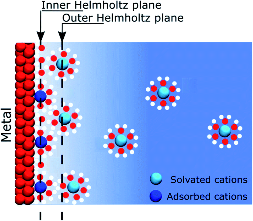Fig. 1 Schematic Stern–Gouy–Chapman representation of a negatively charged metal–electrolyte solution interface. The inner Helmholtz plane corresponds to the position of specifically adsorbed and partially solvated cations, whereas the outer Helmholtz plane corresponds to the plane of closest approach of the hydrated cations.

It should nonetheless be mentioned that as early as 1943, Esin and Shikov,⁷ followed by Erschler in 1946,⁸ studied the so-called discreteness-of-charge effect, when anions are specifically adsorbed and highlighted how localised charges influence the diffuse layer. Following their work, in 1958, Grahame confirmed that the potential generated by two discrete charge layers, as illustrated in Fig. 2, is equal to that of a parallel plate capacitor with smeared charges. However, the potential for a monolayer of discrete charges on an electrode was half that generated by the same charges smeared on a plane due to the presence of image charges (idem at the air–solution interface).⁹ This discreteness-of-charge effect was later shown to be of importance in colloid stability.¹⁰

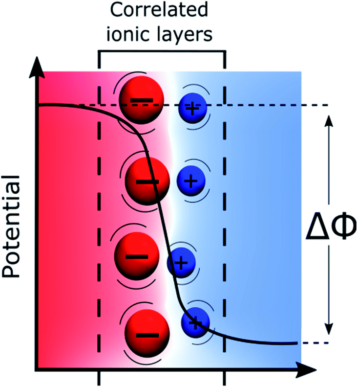Fig. 2 Schematic representation of the double ionic monolayers at the polarised ITIES. Depending on the salts and solvent, the potential difference can reach several hundreds of millivolts. Here, the capacitance of the interface is constant and the surface charge is directly proportional to the applied potential difference across the interface.¹⁴ Ions that do not contribute to the polarisation are not represented.

Another example of defectless and easily reproducible polarisable interface is the “interface between two immiscible electrolyte solutions” (ITIES) as recognised at an early stage by Nernst and Riesenfeld in 1902.¹¹ Here, the system is composed of an aqueous solution of hydrophilic salts – e.g. LiCl – in contact with an immiscible solution of organic solvent and salts. If the salts are either sufficiently hydrophilic or hydrophobic, the system can be considered as ideally polarisable before ions start crossing to the adjacent phase. In this respect, the early attempts to describe the structure of the polarised ITIES were adapted mutatis mutandis from those of the electrode–electrolyte interface. Indeed, the concept of two back-to-back diffuse layers was based on the early work of Vervey–Niessen,¹² Gavach et al.,^13–15 and many others.¹⁶ These models were, however, of limited agreement with the experimental observations.¹⁶

The key problem of the back-to-back diffuse layers model of the ITIES was the difficulty in understanding how the potential distributed across these two adjacent diffuse layers, i.e. across a few nanometres, could act as a driving force for potential dependent ion transfer reactions, and more importantly for potential dependent electron transfer reactions. Indeed, if we consider, say an aqueous oxidised species and an organic reduced species reacting at the interface, how could “this encountering redox pair” sense the potential drop between the two phases? This question has raised a long debate that cannot be settled without a consistent theory of the structure of the polarised ITIES.¹⁷

Discrete Helmholtz model

Discrete Helmholtz model at liquid–liquid interfaces

Recently, using both a simulation approach and experimental measurements including surface second harmonic generation, surface tension measurements and high-frequency capacitance measurements, we have proposed that the potential distribution at liquid–liquid interfaces could be visualised by a “Discrete Helmholtz” model as shown in Fig. 2.^18,81 The gist of this model is that the interface can be viewed as two face-to-face ionic monolayers forming an interfacial ionic capacitor, such that the entire potential drop between the two immiscible phases occurs across a very thin layer, less than one nanometre in thickness.

The major difference between the “Discrete Helmholtz” and the “Gouy–Chapman” models of the liquid–liquid interface can be seen in the capacitance. Whereas the former predicts a constant capacitance, the latter predicts a potential dependent one. A central argument of the “Discrete Helmholtz” approach at an ITIES is that the large bulky organic ions at the interface act as “anchoring points” for the smaller, more mobile aqueous counter ions, thereby favouring ion–ion correlations. Furthermore, this correlation between the ionic layers is enhanced by the fact that the permittivity of water at the interface is much smaller than that in the bulk.^18,19 Indeed, for instance, the water dielectric constant is estimated to be roughly six for the mercury–water interface.²⁰ The reduced permittivity is now well documented^21–23 and is due to the lower variance of the orientation of the dipoles of the water molecules at the interface, which is explained in the framework of the Kirkwood–Fröhlich equation.²⁴ This formalism, however, does not take into account of the presence of external electric fields and mainly depends on the variance of the total dipole moment within the solvent phase. In this respect, Booth extended this approach to include effects of electric fields and found that a reduction of the dielectric constant, because of saturation, already took place at field intensities of 0.1 V nm⁻¹, i.e. at orders of magnitudes relevant to the present discussion.^25,26 Nevertheless, Trasatti has observed that the permittivity of water at a metallic interface was also proportional to the affinity of this metal for oxygen.²⁷ Thus, his results showed that a stronger interaction between the metal and the water molecules actually increases the orientation polarizability of the interfacial dipoles. Furthermore, the correlation between the electronegativity of the metals and the permittivity of the water demonstrated that the latter was a function not only of the orientation of the solvent molecules but also of the magnitude of the dipoles. This is discussed extensively by Conway & Bockris.²⁸

Briefly, the “Discrete Helmholtz” model can be summarised by two simple equations that govern the physics of a planar capacitor. The first expresses that the charge, Q, at the interface is directly proportional to the applied Galvani potential difference, Δϕ, illustrated in Fig. 2:

Q = CΔϕ (1)

The second is linked to the geometry of the interface and expresses the constant capacitance C as a function of the local dielectric constant ε, with, for a planar surface:

C = εS/d (2)

where S is the surface area and d the average distance between the correlated ions.

Therefore, when one polarises a liquid–liquid interface, either with a potentiostat or by distributing a salt, we fix the applied potential difference, that in turn fixes the interfacial charge. This situation is also encountered, for instance, when a liquid–liquid interface is polarised by the partitioning of a “common ion” balanced by hydrophobic and hydrophilic counter-ions²⁹ in the adjacent phases.

The “Discrete Helmholtz” model provides simple explanations to some of the long-standing questions concerning electrochemistry at polarised ITIES. For instance, the “shuttle mechanism” for the ion transfer reactions proposed by Mirkin et al. naturally fits the “Discrete Helmholtz”, in the sense that correlated ions are crucial in both theories.³⁰ Similarly, it solves the question of the shape of the potential distribution at these interfaces – as the potential profiles are less than one nanometre sharp – and thus explains the potential dependence of the electron transfer reactions, since redox pairs located on both sides of the interface would sense the full Galvani potential difference, Δϕ.

Nevertheless, the “Discrete Helmholtz” model also brings new interrogations that would need to be addressed in future studies. One of them, which still concerns the electron-transfer mechanism, is that of the potential difference sensed by a redox pair in the plane of the interface. Indeed, if the “Discrete Helmholtz” model predicts that the potential profiles are sharp perpendicularly to the interface, it also predicts inhomogeneous potential distributions parallel to the interface, as schematically shown in Fig. 3. It thus follows that interfacial redox pairs would have a different reactivity depending on their proximity to a correlated electrolyte pair. This was previously suggested in 1973 by Fawcett and Levine and recently discussed by Goldsmith et al. who showed the microscopic inhomogeneity of the electric field close to a molecule adsorbed on an electrode.^31,82 Another mechanism by which the correlated electrolytes could be involved in the redox reaction would be by stabilisation of the reactive species, as is observed for instance with potassium ions in the case of CO₂ reduction³² or lithium in H⁺ reduction in aprotic solvents.³³ In this case, the electrolytes would play a double role, on the one hand, by inducing a potential difference at the interface, displacing therefore the reaction equilibrium towards the products formation, but on the other hand, by lowering the activation energy of the reaction. More speculatively, the presence of strong electric fields at the interface could be used to catalyse non-redox reactions, as recently suggested.^34,35

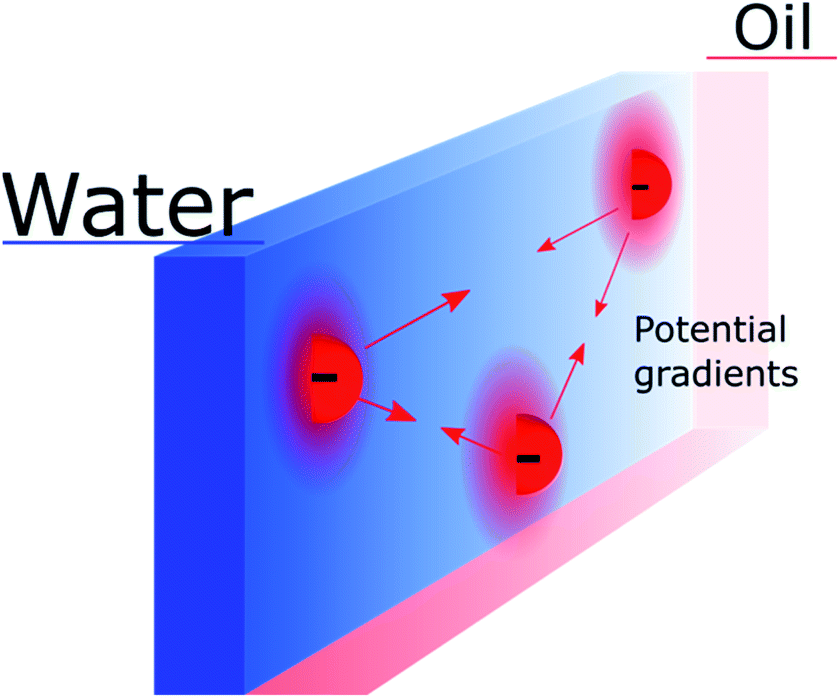Fig. 3 Schematic representation of inhomogeneous potential distribution in the plane of the interface due to the discreteness of the “anchoring points”. The mobile counter ions are not shown.

Discrete Helmholtz model at solid oxide–electrolyte interfaces

To follow the concept of the discreteness of interfacial charges, we have hypothesised that for the interfaces where ionic charges are present, such as metal oxides or silica, the discrete charges act as “anchoring points” where specific electrostatic interactions take place. Furthermore, we observed at the ITIES, that the strength of the interactions between the electrolytes is not high enough so that we could consider ions of opposite charges as being paired. For instance, the ions conserve a mobility in the plane of the interface. In this respect, we prefer to use the term “correlated ions” rather than “ion pairs”.

As previously stated, many solid interfaces present charge inhomogeneity at the molecular scale, for instance silica, which has many applications in electrokinetic phenomena such as electro-osmosis. It has been shown that, for basic solutions, most of the potential drop at a charged silica surface occurs close to the solid in what is often referred to as the “Stern layer” (although there is no specific adsorption of ions as postulated by Stern), between deprotonated silanol groups and non-specifically adsorbed counter cations.^36,37 In this case, the negatively charged silanolates act as “anchoring points” for the mobile cations (Fig. 4).

Fig. 4 Schematic representation of a discrete charge distribution at silica–basic electrolyte interface. Here, the anionic surface charge is solely determined by the pH of the solution thereby fixing the potential drop at the interface assuming a constant capacitance. The shear plane shows the limit between mobile and immobile layers, the arrows show the steady-state velocity of the ions resulting from electrostatic forces in the presence of a viscous drag.

An important aspect to consider here is that since silica is an insulator, the negative charges are localised and the interactions are actually not taking place between the surface of the silica and the electrolytes, but between charged groups and the ions of the electrolyte. Consequently, the potential difference does not take place between the solid and liquid phases, as often illustrated in textbooks,¹⁰ but between two discrete groups having a size comparable to that of a molecule. With this in mind, it becomes questionable to describe the solid surface as a homogeneous and featureless block of constant potential, as also recently discussed by Dufrêche et al. who described the Stern layer of such systems as “a set of attracting points giving rise to contact ion pairs”.³⁸

In summary, we can say that at the solid oxide – solution interface, the surface charge is determined by the pH of the solution due to the amphoteric nature of the fixed charge that in turn determines the potential drop at the interface according to eqn (1), where Δϕ is now the potential drop across the interfacial capacitor.

If the “Discrete Helmholtz” model is appropriate to describe silica surfaces in solution, a key question in the context of electrokinetic phenomena (electro-osmosis, electro-phoresis, etc.) concerns that of the position of the shear plane (slip plane) when an electric field is applied parallel to the interface. Indeed, this plane is classically defined as close to the limit between the inner and outer Helmholtz plans, that is, close to the point where the “Stern layer” becomes the diffuse layer. The argument states that if the potential totally drops in the Stern layer, there is no diffuse layer, therefore there is no shear plan and consequently no electro-osmosis. In this respect, the interface structure depicted by the “Discrete Helmholtz” model brings two interesting elements of an answer. The first is that, as described above, the correlated ions at the charged interface are still mobile in the plane parallel to the interface; they can therefore take part in the ionic current generating the flow. However, the significant viscoelectric effect induced by the solid complicates the response of the ions to the driving electric field.³⁹ The second point is that the distinction between Stern and diffuse layers appears unnecessary, as already suggested by Cooper and Harrison in 1977.^40,41 Thus, in the framework of the “Discrete Helmholtz” model, the diffuse part of the double layer has to be seen more as ions temporarily escaping the attractive potential of the “anchoring points” than as a layer of free ions, distinct from those adsorbed at the interface. As for the zeta potential, this value stems from the classical model with a clear separation between a static “Stern layer” and a mobile diffuse layer. Therefore, in the framework of the “Discrete Helmholtz” model, it cannot be defined further than a proportion of the total potential drop.

Recently, using X-ray photoelectron spectroscopy, Brown et al. observed that for alkali chloride salts, only 10–15% of the potential drop actually takes place in the “diffuse layer”.^36,37 They also rationalised the change of surface potential with aqueous ionic strength by a compression of the double layer.³⁶ Using the same approach, Gmür et al. observed that the co-ions were excluded from the negatively charged interface, implying that cations were responsible for the change of surface properties.⁴² These observations were also confirmed by Jalil & Pyell, using electrokinetic data.⁴³ It has to be noted that the fraction of the potential that drops in the “Stern layer” is inversely proportional to the relative permittivity of the interface. Thus, compared to a polarised ITIES where nearly all the potential drops between the correlated ionic monolayers, only a large fraction of the total potential drops at the silica–water interface, indeed the relative permittivity of the interfacial layer is not as low as for the ITIES (around 45 at the silica–water interface²³vs. 15 at the water–DCE interface¹⁸).

A major difference between metallic and poorly conducting oxide surfaces from an electric viewpoint is the diffuseness of the charge distribution on the metal compared to the discreteness nature at oxide surfaces, because the former are conductors while the latter are often insulators. Consequently, we would argue that the diffuse aspect of the diffuse layer at metallic interfaces, which are described by the Gouy–Chapman model, stems not only from the electrostatic ion–ion interactions taken into account in the Poisson–Boltzmann equation, but also from the diffuseness of the electronic charge at the surface. In the case of oxide layers, the localisation of the charge may favour a “Discrete Helmholtz” model approach where the ionic charges on the solid serve as anchoring points for the counter ions in solution as shown in Fig. 5.

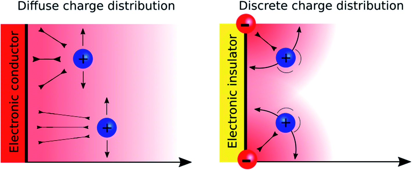Fig. 5 Schematic representation of ion correlation at electronic conductor (left) and insulator (right) interfaces. In the case of an insulator, the probability of finding an ion close to another ion increases. On the left, the capacitance is concentration dependent, on the right it is constant.

Discrete Helmholtz model and porous material for energy storage and geochemistry

The discrete charge correlation described in the “Discrete Helmholtz” model can be extended further to mesoporous materials, where the scale of the electrode features becomes comparable to that of molecular ions, i.e. a few nanometres. This situation is encountered for instance in supercapacitors, where a large specific surface area is needed to increase the energy storage capacities of these devices. Similar to silica–electrolyte interfaces, supercapacitors are often based on oxides such as cobalt oxides or titanium oxides. These compounds are insulators and become conductors only upon oxidation⁴⁴ or reduction.⁴⁵ Their complex current–potential responses have often led some authors to describe them as “pseudocapacitors”, although this concept is now debated with authors claiming⁴⁶ or criticising its relevance.⁴⁷ Indeed, these mesoporous systems actually behave as regular capacitors after an initial faradaic response corresponding to the building of a conductive band in the solid. Thus, at potentials where they are still insulators, it is to be expected that, similarly to silica–water interfaces, their electrical double layer could be described by a single layer of the “Discrete Helmholtz” model. In this case, the potential drop at the insulator–electrolyte interface would take place between the fixed charges and the correlated ionic layer, before the insulator becomes a conductor and the potential profile be described by other models, where the meso and nanoporous structures of the solid play an important role.^48,49 Nevertheless, the constant capacitance of some supercapacitor materials exhibited by their nearly square current potential curves (Fig. 6)⁵⁰ would suggest that the “Discrete Helmholtz” model is appropriate for these materials.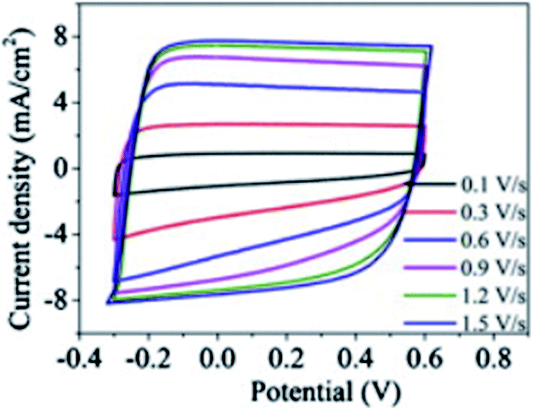

Fig. 6 Example of nearly square current–potential responses of a supercapacitor material (hydrogen-doped TiO₂ nanotubes). The curves were recorded at different scan rates. Reprinted with permission from ref. 50.

In the field of geochemistry, the “Constant Capacitance Model” (CCM), proposed by Schindler & Kamber in 1968, is a model applied to the description of ion intercalation in layered or porous materials.⁵¹ As expected, it assumes a constant capacitance of the solid–electrolyte interface. Initially developed for silica, it has been extended to other amphoteric substrate such as alumina or iron oxides⁵² and generally provides accurate results for various types of ions and solids.^53,54 Beside the constant capacitance, the key aspect of the CCM is that it relies on various equilibrium constants that describe the surface–ion interactions. In this respect, the CCM is similar to the “Discrete Helmholtz” model in that it describes the ions as interacting with specific groups on the solid surface, although the discreteness of the interaction is usually not considered in the CCM.

Recently, intercalation pseudocapacitors have appeared as a way to store energy lying in between batteries, where ions are intercalated in layered substrates, and supercapacitors, where energy is stored by a fast non-faradaic surface reaction.⁵⁵ In this context, the “Discrete Helmholtz” model bridges the conceptual gap between active and passive ion intercalation processes. Thus, in clay minerals or intercalation pseudocapacitors, the solid–electrolyte interface can be described as discrete correlated charge pairs where ions are mobile in the plane of the interface.

Discrete Helmholtz model and the pH glass electrode

An interesting question that follows the above discussion is that of an oxide layer in between two electrolyte solutions, as presented in Fig. 7. If the oxide is glass, such a configuration is that of the classical pH electrodes.⁵⁶ Although pH measurements are perhaps the most widely used analytical techniques the potential response of the glass electrode and their modus operandi are still a matter of debate. The glass electrode is usually described by the ion exchange theory suggested by Nikolsky in 1937 assuming an exchange between cations and protons at the surface of the glass in what is sometimes referred as a glass gel layer.⁵⁷ An alternative explanation based on the so-called adsorption theory was proposed earlier by von Lengyel in 1931 who had studied quartz membrane electrodes and concluded that the potential drop is caused by a difference in the concentration of charge carriers in the “adsorption layer” relative to that in the solution.⁵⁸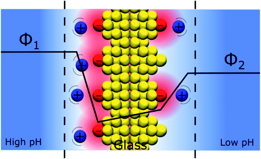

Fig. 7 Schematic representation of a double discrete charge distribution, here at basic pH on both sides, i.e. with a negative surface charge on both sides. In this configuration, different pH values in the solutions separated by the glass layer induce a difference of charged anchoring points and hence a potential difference across the glass layer. The protons are not represented.

Within the framework of the “Discrete Helmholtz” model, we can say that due to the amphoteric properties of the hydrated glass surface, the presence of charges either positive (protonated hydrated group, e.g. –SiOH₂⁺) or negative (de-protonated group, e.g. –SiO⁻) at the surface creates a potential difference between the surface and the bulk on either side of the solid phase. In a glass electrode, the inner compartment has a fixed composition, and a change of pH of the analyte is monitored directly as a variation of the surface polarisation of the glass on the analyte side of about 60 mV/bulk pH. Although this approach considering a difference of surface charges on either side of the glass membrane is an oversimplification of a rather complicated system, where the glass composition is usually not disclosed by pH electrodes manufacturers, it shows how the variation of the bulk pH values in the analyte can be monitored by measuring the difference of potentials between the two solutions separated by an insulator such as a quartz membrane. The same argumentation can be used for pH-FETS (pH sensitive field effect transistors) where a silica gate is deposited on top of a FET.⁵⁹

Discrete Helmholtz model for ion-exchange membranes

Ion exchange membranes (IEM) are widely used in many industrial applications ranging from electrodialysis, to electrolysers and fuel cells.⁶⁰ The ion-exchange membrane – electrolyte solution interface is polarised and the potential difference is classically referred to as the Donnan potential. This voltage results from the competition between the concentration gradient of the mobile ions and the need to maintain the electroneutrality of the inner part of the membrane. The “Discrete Helmholtz” model for an ion-exchange membrane is illustrated in Fig. 8. As for the silica–electrolyte interface, the IEM interface comprises immobile discrete charges in contact with ions in solution. Here, however, the charges in the solid are not only present at its surface but also in its bulk. If IEM are now widely used, it appears that only a few studies are dedicated to the elucidation of the structure of their double layer. In a molecular dynamics simulation of polyamide membrane in contact with a sodium chloride aqueous solution, Kolev & Freger showed that the interaction between the ions and the charged sites in the solid was highly localised and compared the ionic structure as a three dimensional equivalent of the Stern layer.⁶¹ Nevertheless, Galama et al. found that the Donnan model based on the Boltzmann equation yields a good description of the membrane – electrolyte interface, given however that the ion concentration in the membrane was given by interstitial solution volume and not membrane volume.⁶²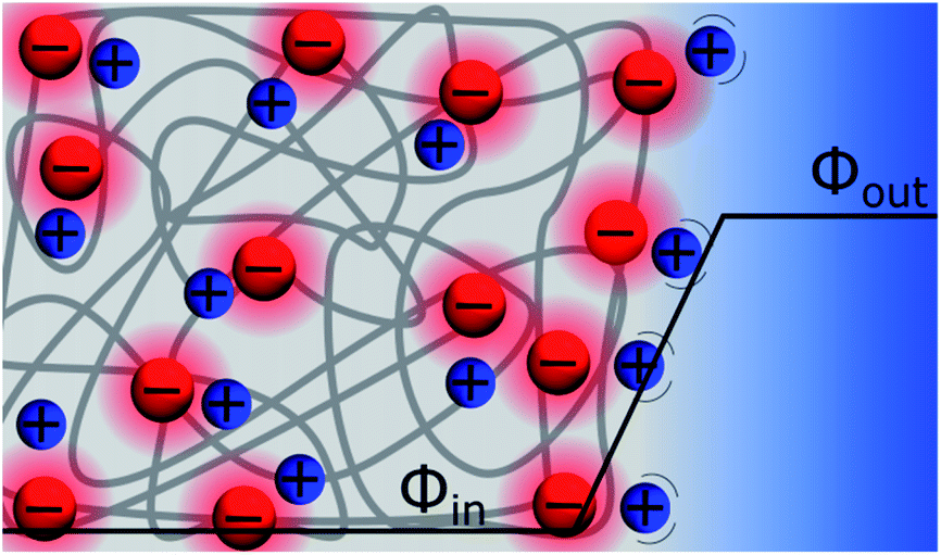

Fig. 8 Schematic representation of an ion-exchange membrane – electrolyte interface. In the framework of the “Discrete Helmholtz” model, the potential drops between two ionic monolayers at the interface.

Discrete Helmholtz model and the bilayer lipid membranes

An interesting aspect of liquid–liquid interfaces is that they have long been considered as model systems to understand the electrical aspects of polarised biological cell membranes, where the Gouy–Chapman model is widely applied⁶³ to describe the charge distribution on either side of the membrane. Indeed, the situation presented in Fig. 9 shows some similarities with these systems, assuming that the insulating silica layer is replaced by the hydrocarbon “tails” of the phospholipids, while the charged SiO⁻ or SiOH₂⁺ groups are replaced by their charged or zwitterionic “heads”.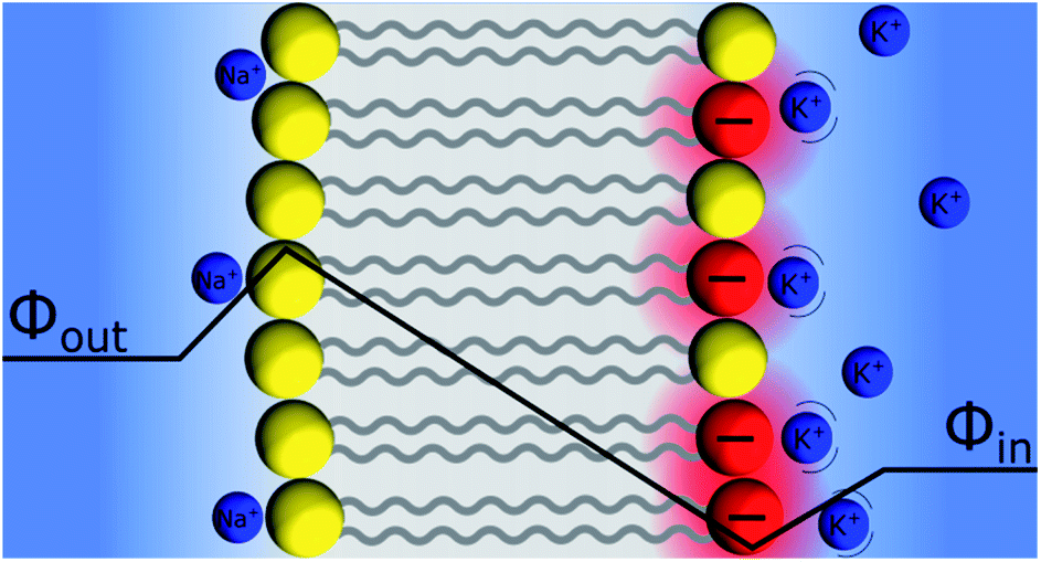

Fig. 9 Schematic representation of a phospholipid bilayer polarisation induced by surface charge asymmetry. The potassium ions inside the cell are “correlated” to the charged phospholipids according to the “Discrete Helmholtz” model, whereas the sodium ions are specifically interacting with the carbonyl groups of the neutral phospholipids. Please note the absence of Gouy–Chapman diffuse layers in this representation. Counter charges are not represented for clarity.

The possibility to create a potential difference between two aqueous layers separated by a hydrophobic solvent with adsorbed charged amphiphilic molecules was studied in 1965 by Colacicco. By injecting small amounts (μM) of sodium dodecylsulfate (SDS) as anionic surfactant or cetyltrimethylammonium bromide (CTAB) as positive surfactant in one of the aqueous phases, a polarisation of +140 mV or −150 mV could be induced across a water–pentanol–water system.⁶⁴ Interestingly, the potential difference decreased with the supporting electrolyte concentration and was dependent on the type of salt used, similarly to what was observed at the silica–water interface by Brown et al.³⁶ In a second study, the same author showed that the same systems could undergo potential inversion of several hundreds of millivolts following a change in the composition of the adsorbed surfactant layer.⁶⁵ Interestingly, Colacicco concluded this work by questioning the possible implications of such a “non-concentration” and “non-diffusion” potential in the polarisation of biological membranes. Recently, Tamagawa et al. showed that it was possible to induce a potential difference across an ion impermeable membrane supporting the idea that membrane polarisation can be generated by controlling the surface charges on both sides of the membrane and discussed its applicability to biomembranes.^66–69

The resting biological membrane potential has been the subject of extensive studies. In most textbooks, it is usually rationalised in terms of the asymmetric distribution of cations between the outside and the inside of the cells, the semi-permeability of the cell membrane and the presence of ion-channel proteins acting as molecular “pumps”.⁷⁰ In this respect, the Goldman–Hodgkin–Katz model based on diffusion–migration expresses the transmembrane potential difference as a function of the relative permeabilities of the different ionic species (Na⁺, K⁺, Cl⁻) and their concentrations.

At the same time, others suggested that the resting potential stems from the asymmetry of the charge distribution of the back-to-back lipid layers, as illustrated in Fig. 9. Indeed, the phospholipid compositions of the inner and outer layers are different. For example, in the human red blood cells, the outer layer is rich in phosphatidylcholine and sphingomyelin, both being zwitterionic, and various glycolipids; the inner layer is rich in phosphatidylethanolamine, phosphatidylserine, both negatively charged, and phosphatidylinositol and their derivatives.⁷¹ As for the glass electrode, the asymmetry of surface charge distribution will result in a potential difference across the bilayer lipid membrane. Furthermore, although the charged lipids are mobile within the membrane, they can nonetheless act as “anchoring points” for the more mobile cationic counter charges inside the cell, mainly potassium. Furthermore, even if the outer lipid layer is rather neutral, the excess of sodium ions outside the cell may cause an ion “binding” between sodium and the carbonyl groups. Indeed, specific binding of sodium cations to zwitterionic phospholipids would yield an overall charged group, further able to polarise the membrane. This situation has been observed by Lee et al. in molecular mechanics simulations of a sodium rich and a potassium rich aqueous phases separated by a symmetric bilayer of phosphatidylcholine.⁷² In this configuration, the binding of sodium ions to the exposed phospholipid layer yielded a potential difference of 70 mV.

In this respect, the nature of the interaction between the charged heads of the phospholipids and the alkali cations is still to be determined. It is known that the extent of binding follows the Hofmeister series, that is, Li⁺ binds more than Na⁺ and Na⁺ more than K⁺,^73,74 which means that the interaction is not only electrostatic. It also appears that the ion binding process is endothermic, though spontaneous, which suggests an entropy driven phenomenon that involves solvent molecules.⁷⁵ However, it is not clear how many phospholipid heads are binding with cations.⁷⁶ Indeed, some studies suggest that cations bind preferentially to oxygen atoms of the carbonyl groups⁷⁷ – similarly to that which is observed for proteins⁷⁸ – while others find no preference for carbonyl or phosphate.⁷⁹ Nevertheless, these differences might actually stem from the different parameters used to simulate these systems by molecular dynamics.⁸⁰

Therefore, biomembranes polarisation can be treated concomitantly by considering the ionic distribution across the membrane and its permeability for the different ions using a diffusion–migration model and by considering an asymmetric charge distribution of the lipids in the bilayer (Fig. 9). It should be noted that these two approaches are not contradictory as both phenomena occur simultaneously, an open question being: what is the driving force to maintain this steady-state polarisation?

The role of oxygen, by maintaining oxidative phosphorylation and glycolysis to produce ATP, which in turn drives the Na⁺/K⁺ ATPase, is key to keeping the cell polarised. The source of the polarisation stems from redox reactions involving proton fluxes thereby driving ion partitioning and membrane polarisation. In other words, we would argue that it is not the membrane structure that fixes the transmembrane polarisation, but rather its respiratory function and the membrane structure that further accommodates this potential difference by an asymmetry of the phospholipid distribution.

Overall, even if polarisation effects in biology are very complex, the “Discrete Helmholtz” model applied to bilayer lipid membranes suggests that all the transmembrane potential difference can occur directly at the membrane, without space charged regions in the adjacent solutions.

Conclusions

In summary, this perspective shows the remarkable similarities in the structures of the electrical “double layers” at various charged insulators – electrolytes interfaces. This similarity stems from the discrete nature of the charge carriers at interfaces which, coupled with the low permittivity of the interfacial medium, allows a large fraction of the interfacial potential drop to take place between two correlated ionic layers. The correlation, however, is not strong enough so that the ions can be considered as adsorbed or immobile; they can therefore take part in the ionic conduction in the plane parallel to the interface. Consequently, these systems do not present a true “double layer” structure, that is, a Stern layer and a Gouy–Chapman layer, but rather a monolayer of correlated ions having a limited degree of freedom in the direction perpendicular to the interface. This monolayer is conceptually different from the Stern layer of the classical model where the ions are specifically adsorbed.

The understanding of polarised interfaces is key to many systems and has a wide range of implications not only in electrochemistry but also in biology. As can be seen above, some complex interfaces such as the glass pH electrodes or the biomembranes are still not yet fully understood. Here, we wish to put forward the concept of ionic “correlations” between fixed charges or slowly moving anchoring points and mobile counter charges. Ion correlation differs from ion paring or from specific adsorption in the sense that the presence of mobile ions around a fixed counter-charge results in local potential differences that may average in the case of flat surfaces.

In the examples discussed here, we illustrate that systems based on electrolyte–insulator–electrolyte interfaces can be polarised if the ionised surface charges present on both sides of the insulator are different. An important aspect of the “Discrete Helmholtz” model is that potential differences at the surface of the insulator layer can take place over very short distances where two face-to-face ionic layers are present.

Conflicts of interest

The authors declare no conflict of interest.

Acknowledgements

The authors gratefully acknowledge the financial support provided by the Swiss National Science Foundation (grant number 175745 entitled Photo Induced Charge Transfer Reaction at Molecular Interfaces: towards new routes of solar energy storage) and the Doctor Pekka Peljo from Turku University for interesting discussions.

References

1. H. Helmholtz, Ann. Phys., 1879, 243, 337–382.
2. S. Arrhenius, Z. Für Phys. Chem., 1887, 1, 631.
3. M. Gouy, J. Phys. Theor. Appl., 1910, 9, 457–468.
4. D. L. Chapman, Philos. Mag., 1913, 25, 475–481.
5. O. Stern, Z. Für Elektrochem. Angew. Phys. Chem., 1924, 30, 508–516.
6. D. C. Grahame, Chem. Rev., 1947, 41, 441–501.
7. O. A. Esin and V. M. Shikov, Zh. Fiz. Khim., 1943, 17, 236.
8. B. V. Ershler, Zh. Fiz. Khim., 1946, 20, 679.
9. D. C. Grahame, Z. Für Elektrochem. Berichte Bunsenges. Für Phys. Chem., 1958, 62, 264–274.
10. R. J. Hunter, Zeta Potential in Colloid Science: Principles and Applications, Academic Press, 2013.
11. W. Nernst and E. H. Riesenfeld, Ann. Phys., 1902, 313, 600–608.
12. E. J. W. Verwey and K. F. Niessen, Philos. Mag., 1939, 28, 435–446.
13. C. Gavach, P. Seta and B. D’epenoux, J. Electroanal. Chem. Interfacial Electrochem., 1977, 83, 225–235.
14. M. Gros, S. Gromb and C. Gavach, J. Electroanal. Chem. Interfacial Electrochem., 1978, 89, 29–36.
15. P. Seta, B. d'Epenoux and C. Gavach, J. Electroanal. Chem. Interfacial Electrochem., 1979, 95, 191–199.
16. G. C. Gschwend, A. Olaya, P. Peljo and H. H. Girault, Curr. Opin. Electrochem., 2020, 19, 137–143.
17. P. Peljo, E. Smirnov and H. H. Girault, J. Electroanal. Chem., 2016, 779, 187–198.
18. G. C. Gschwend, A. Olaya and H. Girault, Chem. Sci. 10.1039/d0sc00685h.
19. J. O. Bockris, M. A. V. Devanathan and K. Müller, in Electrochemistry, ed. J. A. Friend and F. Gutmann, Pergamon, 1965, pp. 832–863.
20. R. Parsons and P. C. Symons, Trans. Faraday Soc., 1968, 64, 1077–1092.
21. V. Vogel and D. Möbius, Thin Solid Films, 1988, 159, 73–81.
22. O. Teschke, G. Ceotto and E. F. de Souza, Chem. Phys. Lett., 2000, 326, 328–334.
23. D. A. Sverjensky, Geochim. Cosmochim. Acta, 2005, 69, 225–257.
24. M. Neumann, Mol. Phys., 1983, 50, 841–858.
25. F. Booth, J. Chem. Phys., 1951, 19, 391–394.
26. F. Booth, J. Chem. Phys., 1955, 23, 453–457.
27. S. Trasatti, J. Electroanal. Chem. Interfacial Electrochem., 1981, 123, 121–139.
28. S. Trasatti, in Modern Aspects of Electrochemistry, ed. B. E. Conway and J. O. Bockris, Springer US, Boston, 1979, pp. 81–206.
29. H. H. Girault, Analytical and physical electrochemistry, Marcel Dekker, Lausanne, Switzerland, New York, 2004.
30. F. O. Laforge, P. Sun and M. V. Mirkin, J. Am. Chem. Soc., 2006, 128, 15019–15025.
31. W. R. Fawcett and S. Levine, J. Electroanal. Chem. Interfacial Electrochem., 1973, 43, 175–184.
32. M. Liu, Y. Pang, B. Zhang, P. De Luna, O. Voznyy, J. Xu, X. Zheng, C. T. Dinh, F. Fan, C. Cao, F. P. G. de Arquer, T. S. Safaei, A. Mepham, A. Klinkova, E. Kumacheva, T. Filleter, D. Sinton, S. O. Kelley and E. H. Sargent, Nature, 2016, 537, 382–386.
33. I. E. Castelli, M. Zorko, T. M. Østergaard, P. F. B. D. Martins, P. P. Lopes, B. K. Antonopoulos, F. Maglia, N. M. Markovic, D. Strmcnik and J. Rossmeisl, Chem. Sci., 2020, 11, 3914–3922.
34. S. Shaik, D. Mandal and R. Ramanan, Nat. Chem., 2016, 8, 1091–1098.
35. F. Che, J. T. Gray, S. Ha, N. Kruse, S. L. Scott and J.-S. McEwen, ACS Catal., 2018, 8, 5153–5174.
36. M. A. Brown, A. Goel and Z. Abbas, Angew. Chem., Int. Ed., 2016, 55, 3790–3794.
37. M. A. Brown, Z. Abbas, A. Kleibert, R. G. Green, A. Goel, S. May and T. M. Squires, Phys. Rev. X, 2016, 6, 011007.
38. S. Hocine, R. Hartkamp, B. Siboulet, M. Duvail, B. Coasne, P. Turq and J.-F. Dufrêche, J. Phys. Chem. C, 2016, 120, 963–973.
39. W.-L. Hsu, H. Daiguji, D. E. Dunstan, M. R. Davidson and D. J. E. Harvie, Adv. Colloid Interface Sci., 2016, 234, 108–131.
40. I. L. Cooper and J. A. Harrison, Electrochim. Acta, 1977, 22, 519–524.
41. I. L. Cooper and J. A. Harrison, Electrochim. Acta, 1977, 22, 1361–1363.
42. T. A. Gmür, A. Goel and M. A. Brown, J. Phys. Chem. C, 2016, 120, 16617–16625.
43. A. H. Jalil and U. Pyell, J. Phys. Chem. C, 2018, 122, 4437–4453.
44. H. Kang, J. Lee, T. Rodgers, J.-H. Shim and S. Lee, J. Phys. Chem. C, 2019, 123, 17703–17710.
45. I. Abayev, A. Zaban, F. Fabregat-Santiago and J. Bisquert, Phys. Status Solidi A, 2003, 196, R4–R6.
46. P. Simon, Y. Gogotsi and B. Dunn, Science, 2014, 343, 1210–1211.
47. C. Costentin and J.-M. Savéant, Chem. Sci., 2019, 10, 5656–5666.
48. P. M. Biesheuvel, Y. Fu and M. Z. Bazant, Phys. Rev. E: Stat., Nonlinear, Soft Matter Phys., 2011, 83, 061507.
49. C. Costentin and J.-M. Savéant, ACS Appl. Energy Mater., 2019, 2, 4981–4986.
50. H. Wu, D. Li, X. Zhu, C. Yang, D. Liu, X. Chen, Y. Song and L. Lu, Electrochim. Acta, 2014, 116, 129–136.
51. P. Schindler and H. R. Kamber, Helv. Chim. Acta, 1968, 51, 1781–1786.
52. S. Goldberg and G. Sposito, Soil Sci. Soc. Am. J., 1984, 48, 772–778.
53. S. Goldberg, S. M. Lesch and D. L. Suarez, Soil Sci. Soc. Am. J., 2002, 66, 1836–1842.
54. S. Goldberg, Vadose Zone J., 2004, 3, 676–680.
55. Y. Liu, S. P. Jiang and Z. Shao, Mater. Today Adv., 2020, 7, 100072.
56. D. J. Graham, B. Jaselskis and C. E. Moore, J. Chem. Educ., 2013, 90, 345–351.
57. B. P. Nikolsky, Zh. Fiz. Khim., 1937, 10, 495.
58. B. v Lengyel, Z. Phys. Chem., Abt. A, 1931, 153, 425–442.
59. P. Bergveld, IEEE Trans. Biomed. Eng., 1970, 17, 70–71.
60. J. Ran, L. Wu, Y. He, Z. Yang, Y. Wang, C. Jiang, L. Ge, E. Bakangura and T. Xu, J. Membr. Sci., 2017, 522, 267–291.
61. V. Kolev and V. Freger, J. Phys. Chem. B, 2015, 119, 14168–14179.
62. A. H. Galama, J. W. Post, M. A. Cohen Stuart and P. M. Biesheuvel, J. Membr. Sci., 2013, 442, 131–139.
63. L. P. Savtchenko, M. M. Poo and D. A. Rusakov, Nat. Rev. Neurosci., 2017, 18, 598–612.
64. G. Colacicco, Nature, 1965, 207, 936–938.
65. G. Colacicco, Nature, 1965, 207, 1045–1047.
66. H. Tamagawa, M. Funatani and K. Ikeda, Membranes, 2016, 6, 11.
67. H. Tamagawa and K. Ikeda, J. Biol. Phys., 2017, 43, 319–340.
68. H. Tamagawa and K. Ikeda, Eur. Biophys. J., 2018, 47, 869–879.
69. T. Heimburg, Eur. Biophys. J., 2018, 47, 865–867.
70. A. J. Bruce Alberts, J. Lewis, D. Morgan, M. Raff, K. Roberts and P. Walter, Molecular Biology of the Cell, Taylor & Francis Group, Garland Science, 6th edn, 2015.
71. T. Fujimoto and I. Parmryd, Front. Cell Dev. Biol., 2017, 4, 155.
72. S.-J. Lee, Y. Song and N. A. Baker, Biophys. J., 2008, 94, 3565–3576.
73. P. Jurkiewicz, L. Cwiklik, A. Vojtíšková, P. Jungwirth and M. Hof, Biochim. Biophys. Acta, Biomembr., 2012, 1818, 609–616.
74. P. Maity, B. Saha, G. S. Kumar and S. Karmakar, Biochim. Biophys. Acta, Biomembr., 2016, 1858, 706–714.
75. B. Klasczyk, V. Knecht, R. Lipowsky and R. Dimova, Langmuir, 2010, 26, 18951–18958.
76. E. Deplazes, J. White, C. Murphy, C. G. Cranfield and A. Garcia, Biophys. Rev., 2019, 11, 483–490.
77. R. A. Böckmann, A. Hac, T. Heimburg and H. Grubmüller, Biophys. J., 2003, 85, 1647–1655.
78. L. Vrbka, J. Vondrášek, B. Jagoda-Cwiklik, R. Vácha and P. Jungwirth, Proc. Natl. Acad. Sci. U. S. A., 2006, 103, 15440–15444.
79. A. Cordomí, O. Edholm and J. J. Perez, J. Phys. Chem. B, 2008, 112, 1397–1408.
80. A. Cordomí, O. Edholm and J. J. Perez, J. Chem. Theory Comput., 2009, 5, 2125–2134.
81. G. C. Gschwend and H. Girault, J. Electroanal. Chem., 2020, 872C, 114240.
82. Z. K. Goldsmith, M. Secor and S. Hammes-Schiffer, ACS Cent. Sci., 2020, 6, 304–311.

---