Molecular dynamics based descriptors for predicting supramolecular gelation

Abstract

Whilst the field of supramolecular gels is rapidly moving towards complex materials and applications, their design is still an effortful and laborious trial-and-error process. Herein, we introduce four new descriptors that can be derived from all-atom molecular dynamics simulations and which are able to predict supramolecular gelation in both water and organic solvents. Their predictive ability was demonstrated via two separate machine learning techniques, a decision tree and an artificial neural network, with a dataset composed of urea-based gelators. Owing to the physical relevance of these descriptors to the supramolecular gelation process, their use could be conceptualized to other classes of supramolecular gelators and hence steer their design.

---

Introduction

In recent years, Low Molecular Weight Gelators (LMWGs) have attracted significant attention. Currently, the field is focussed on developing efficient supramolecular gels for various specialized applications, ranging from drug delivery systems to catalyst templates or even optoelectronic applications.^1–3 Despite two decades of intense research on supramolecular gelators, their discovery remains surprisingly reliant on serendipity, due to the sensitivity of the supramolecular gelation process towards small molecular changes of the LMWG.^4–6 In this context, multiscale computational methodologies have the potential to provide a better understanding of the underlying relationship between the molecular structure and the gelation ability.⁷ However, besides post-rationalization, the ability to predict supramolecular gelation by means of computational methods has been scarcely explored.

The first predictive tool for organogel formation was reported in 2011 by Raynal and Bouteiller.⁸ In their pioneering work, Hansen Solubility Parameters (HSPs) were employed to define solubility and gelation spheres in Hansen space by means of an elaborate assessment of the behaviour of a known Low Molecular Weight Gelator (LMWG) in several solvents. Based on these spheres, the gelation performance of the LMWG in an untested solvent could then be predicted using the HSPs of this new solvent. If the HSP values fall inside the solubility sphere or the gelation sphere, it is likely that the LMWG will, respectively, be soluble or form a gel in the solvent. Follow-up works from the group of Bouteiller further improved the quality and scope of this method to determine the gelation domain from the solubility data of LMWGs.^9,10 This approach, however, still requires the synthesis of the molecule and an extensive gelation screening beforehand, as for each new LMWG, solubility data needs to be gathered to define the gelation domain. Furthermore, the reliability of the prediction depends on the quality of the initial solubility data set.⁸

The combined effort of the Tuttle and Ulijn groups resulted in the development of a predictive method for the self-assembly properties of tripeptides in water based solely on computations.^11,12 Using high throughput coarse-grained molecular dynamics simulations, a hydrophobicity-corrected aggregation propensity score (AP_H) could be obtained, which originates from the solvent accessible surface area of the aggregate as well as the partitioning coefficient (log P) of the gelator.¹³ By screening the AP_H score of 8000 tripeptides in water, they were able to bring forth a set of design rules to promote aggregation and supramolecular hydrogelation. As their method focuses on the hydrogelation of tripeptide gelators, the applicability to non-peptide gelators requires a specialized coarse-grained model. Recently, Adams and Berry developed a machine learning model to successfully predict the hydrogelation propensity of functionalised amino acids and dipeptides using physicochemical properties and molecular fingerprints.¹⁴ Descriptors such as the number of rings, polar surface area, solvent accessible surface area and log P emerged as key parameters for predicting gelation, together with a number of molecular fingerprint descriptors, which are abstract and difficult to interpret. An added value of such approach is that it can be offered via an online interface, since only a SMILES code is needed as input to obtain a prediction of the hydrogelation properties of the molecule. Moreover, next to the prediction itself, the relevancy of the prediction is indicated. The predictions are accurate as long as the molecule falls within the applicability domain of the model, defined by the properties of the amino acids and dipeptides present in the training set. To recreate a similar predictive model for non-peptide gelators that currently fall outside the applicability domain of their prediction model, a significant amount of new data is required.

Among the different types of LMWGs, peptide-based hydrogelators belong to one of the best represented classes of gelators due to their potency in several biomedical applications.^15,16 While they benefit from biocompatibility, their synthesis is often costly and time consuming. In contrast, the class of urea-based gelators enjoy a cheap and straightforward synthesis allowing easy derivatization. Recently, we reported on a thixotropic and cytocompatible bis-urea derivative with potential in biomedical applications.¹⁷ In this work, we set out to develop a conceptual molecular dynamics guided predictive model for urea-based supramolecular gelation to improve their current empirical design strategy. In essence, we aim for an approach fulfilling the following four criteria: (i) the method should be able to correctly predict supramolecular gelation of urea-based molecules by means of computations exclusively. (ii) Instead of a binary yes/no answer, the outcome of the predictions should be a three-level categorical response: gel, precipitate and solution. (iii) Only descriptors with a physical relevance towards supramolecular gelation should be used to build the model, in order to provide chemical insights into the structure–gelation relationships. With suitable descriptors, the approach could be conceptualized to other supramolecular gelator classes. (iv) And finally, the predictions should be accurate in both water (hydrogelation) and organic solvents (organogelation) (Fig. 1).

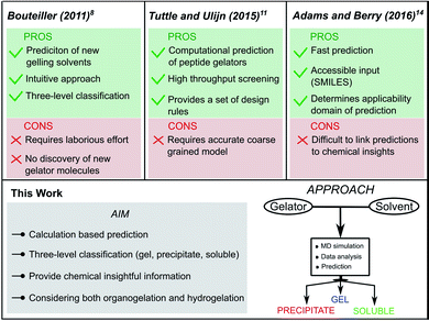Fig. 1 Comparison of reported supramolecular gelation predictive models with the approach followed in this work.

Methodology

The dataset

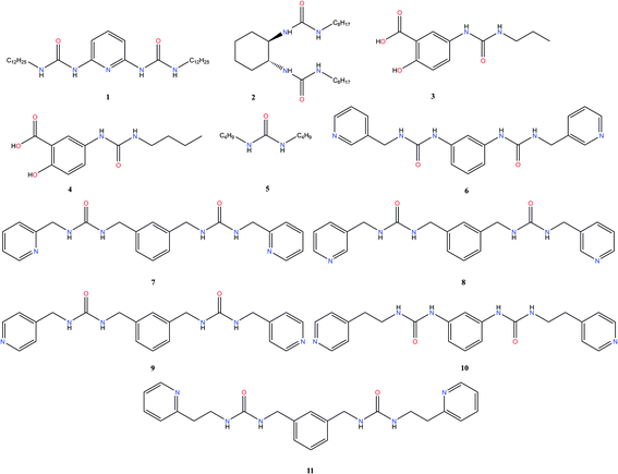
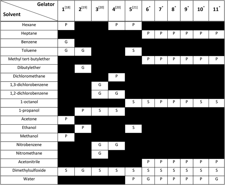
To construct the model and test the predictive ability of our approach, a library of urea-based LMWGs was generated, which is shown in Fig. 2. Some LMWGs were previously reported by other research groups (1, 2, 3, 4 and 5), while other compounds were recently synthesized by our group (6, 7, 8, 9, 10 and 11).^7,17–21 The compounds were selected on the basis of two criteria. First, the molecule should contain at least one urea moiety. Second, the experimental protocol to assess the gelation performance in a certain solvent should be exactly the same for all compounds. It is crucial to fulfil the latter criteria in order for the data to be consistent, since the gelation procedure significantly affects the gelation propensity.²² This imposes serious restrictions on the data available in literature on urea-based LMWGs that can be used in this study, as gelation procedures often vary or are ill-defined. Herein, all compounds have been screened for their gelation ability based on the same procedure, involving a heating and cooling cycle to obtain the gel at a concentration of LMWG smaller or equal than 1.0% w/v. The full library contains non-gelators, organogelators as well as hydrogelators. A total of 65 data points has been obtained by screening the gelation performance in different solvents. For compound 1–5, gelator–solvent combinations were selected based on available literature data keeping diversity in gelation properties in mind.^17–21 Whilst data on compound 6–11 was generated by our own experiments, with solvents being selected based on their difference in polarity and hydrogen bonding capabilities. Although the size of this dataset is modest, previous studies in different fields have shown to deliver a promising predictive model with similar dataset sizes, by using models with a low complexity or by means of chemically relevant descriptors.^14,23,24

Fig. 2 Urea-containing Low Molecular Weight Gelators contained in the dataset used in this work.

Molecular dynamics

In our previous work on the rationalization of supramolecular hydrogelation through a multiscale computational approach, we have showed that all-atom molecular dynamics simulations, emerge as a unique tool to provide insight into the aggregation phase during supramolecular gelation.⁷ Similarly, in the pioneering work of Tuttle and Ulijn,¹¹ coarse grained molecular dynamics was applied to obtain their AP_H score and predict the hydrogelation performance of tripeptides. Herein, molecular dynamics simulations are performed to obtain a set of descriptors, which we envisioned to have predictive ability value in supramolecular gelation. The MD simulations were performed by placing 5 gelator molecules in a periodic cubic box filled with solvent molecules to reach a concentration of 1.0% w/v. The same concentration is used in the experimental determination of the gelation performance. A trajectory of 50 ns with a timestep of 0.5 fs was gathered using the CHARMM27 force field, with the parameters retrieved from the Swissparam service.^25,26 This force field was already shown to accurately describe urea based interactions, which are key during the supramolecular gelation of urea containing compounds.^7,27 Before production, an energy minimization and temperature/pressure equilibration step was performed to ensure steric clashes or inadequate equilibration of the NPT-ensemble would not affect the production simulation. The V-rescale thermostat and Parrinello–Rahman barostat were used with the temperature set at 300 K and the pressure at 1.0 bar.²⁸ All molecules were randomly placed inside the simulation box with the gelator molecules separately being dispersed in the solvent, using the Packmol software, while simulations were run with the Gromacs software version 2018.3.^29,30 All descriptors were obtained as a time average over the 50 ns simulation, with a snapshot taken every 2.5 ps. A detailed description of the methodology can be found in the ESI (S3†).

Descriptors for supramolecular gelation

For a molecule to act as an efficient low molecular weight gelator, a number of criteria needs to be met: (i) the molecule should have a suitable solvophobic balance, (ii) it should contain sites for non-covalent interactions allowing the formation of a reversible network and (iii) these non-covalent interactions should promote the anisotropic growth of a Self-Assembled Fibrillar Network (SAFiN) that immobilizes the solvent and causes the distinct supramolecular gel features.³¹ Four MD generated descriptors are introduced in this work that quantify one or more of these criteria and thus could have the ability to predict supramolecular gelation.

Relative solvent accessible surface area (rSASA). The Solvent Accessible Surface Area (SASA) is defined as the total area of a molecule that is accessible to the solvent. If unfavourable interactions are present between the molecule and its solvent, the molecule will tend to decrease the contact area with the solvent by aggregation and as a result a small SASA is observed (Fig. 3B). As such, the SASA is associated with the solvophobic balance of the molecule under investigation and its intermolecular aggregation. Tuttle and Ulijn use the SASA to determine their aggregation propensity score, as previously mentioned.¹¹ In this work, a relative Solvent Accessible Surface Area (rSASA) is introduced, which is computed by dividing the time-average of the combined SASA of the gelator molecules during the 50 ns simulations with a maximum SASA (SASA_max). The latter is obtained by multiplying the SASA of a single fully extended gelator molecule (i.e. all dihedral angles of the backbone are set to 180°) with the number of gelator molecules present in the simulation box.

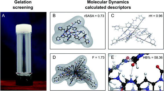Fig. 3 Schematic representation of the experimental gelation screening (A) and the computation of the four descriptors rSASA, rH, F and HB% from a molecular dynamics simulation (B–E).

By taking the time-averaged value of the SASA instead of the SASA of the final frame of the simulation, a robust score is obtained important for small scale all-atom simulations. The and SASA_max are computed by the double cubic lattice method with the radius of the solvent probe set at 1.4 Å.³² Values close to 1 of the rSASA descriptor indicate absence of aggregation, while values significantly smaller than 1 indicate solvophobic interactions triggering aggregation.

Relative end-to-end distance (rH). In our previous work, we showed how the end-to-end distance is a valuable descriptor to define the shape of a single gelator molecule.⁷ To assess the effect that the solvent environment, other gelator molecules and intramolecular interactions have on the shape of the gelator molecule, a relative end-to-end distance (rH) is defined, which is computed by measuring the average distance between the most distant atoms of the backbone over time in all gelator molecules present in the simulation (R̄) and dividing this value with the maximum end-to-end distance, obtained by measuring the distance between the respective atoms of a corresponding fully extended molecule (R_max) (Fig. 3C).

Similarly, it is rationalized that, if sufficient rotatable bonds are present in the molecule, the rH descriptor evaluates the interactions between the gelator molecule and the environment. If the molecule has pronounced solvophobic interactions, it will decrease its contact with the solvent resulting in a collapsed shape and a decreased value of rH. Therefore, rH can be regarded as a measure for intramolecular aggregation. Nevertheless, it is important to note that, next to gelator/solvent interactions, intramolecular and intermolecular gelator/gelator interactions could also have a pronounced effect on the value of rH. Indeed, upon self-assembly of the gelator molecules to a nanofiber, one can assume that in the centre of the fiber, the gelator molecules are mainly surrounded by other gelator molecules. While at the surface, the gelator molecules are in contact with solvent molecules and here solvent–gelator interactions need to be taken into consideration. As molecules are constantly moving during the simulation, it is not straightforward to make a clear differentiation between molecules located in the centre of the aggregate or at the surface. For this reason, the average is taken over all gelator molecules in the simulation. Additionally, the flexibility of the gelator molecule will have an effect on the value of this descriptor, as molecules with no or little rotatable bonds in their structure will have an almost constant value of rH irrespective of the solvent.

Hydrogen bonding percentage (HB%). The urea moiety has unique hydrogen bonding characteristics, being able to act as a hydrogen bond donor as well as a hydrogen bond acceptor. Hydrogen bonding between urea moieties resulting in a urea α-tape motif is an important factor in the anisotropic fibre formation and gelation process of urea-based supramolecular gels.³³ However, previous work indicates other types of hydrogen bonding interactions, such as hydrogen bonding between a urea and a pyridyl moiety, to influence the gelation performance in these gelators as well.^7,34,35 With this in mind, the hydrogen bonding percentage descriptor (HB%) is introduced to quantify the non-covalent intermolecular interactions that connect the gelator molecules (Fig. 3E). To calculate the HB%, first all classical hydrogen-bond donors (NH, OH, SH, …) and acceptors (O, N, F, …) in the molecule are identified. Next, the sum is taken over every intermolecular connection between a hydrogen bond donor atom (i) and a hydrogen bond acceptor atom (j) over every time step (N) of the simulation. A connection is deemed present when the distance between the donor and acceptor atom is below 3 Å. This distance was selected based on hydrogen bond distances observed in an interaction library, containing a variety of urea-based hydrogen bonding interactions.⁷ This sum is divided by the total number of time steps in the simulation and multiplied by 100% to get the final HB% value. As such, the HB% descriptor is closely linked to the native contact analysis applied to study protein folding.³⁶ Note that bifurcated hydrogen bonds are counted as a single connection during the analysis, as either one acceptor or one donor atom is involved (i.e. for a certain time step N and a certain value of i or j, the value of t_ij cannot exceed 1).

Shape factor (F). While the above descriptors provide information concerning the solvophobic balance and non-covalent interactions of the gelator molecules, it is essential to be able to quantify the shape of the aggregate. For this reason, we present a shape factor (F) that can be calculated by taking the ratio of a time averaged computed radius of gyration to a pseudo hydrodynamic radius , similar to the particle shape factor used in the field of proteins and polymers (Fig. 3D).³⁷ is calculated as the square root of the mass averaged distance of all gelator atoms (A) to the centre of mass of all gelator atoms in the simulation. Classically, the hydrodynamic radius R_h of a particle is measured by dynamic light scattering experiments and is defined as the radius of a hypothetical hard sphere that will diffuse with the same speed as the solvated particle under investigation.³⁷ Based on this, a computable pseudo hydrodynamic radius is suggested as the radius of a hypothetical hard sphere that has the same volume as the combined molecular volume of all gelator molecules (V_gel). The latter can be approximated by calculating the volume of a single extended gelator molecule using the double cubic lattice method with the probe radius set to 1.4 Å and multiplying this value with the total number of gelator molecules present in the simulation. The purpose of the shape factor F lies in the description of the shape of the aggregate that is observed during the molecular dynamics simulation. When the aggregate has a spherical shape a low value of F is computed, when the aggregate adopts a more fibrous shape, F increases.

The descriptors defined above can all be calculated based on data generated in a molecular dynamics simulation and by employing the open-source GROMACS software (version 2018.3) together with its implementations.²⁹ A detailed explanation on the practical aspects to obtain the descriptors is provided in the ESI (S4–S7†).

Results and discussion

Gelation results

A thorough gelation screening in multiple solvents was already performed on some of the urea-based compounds in our library (1, 2, 3, 4 and 5), making the classification of data associated with these compounds straightforward (Fig. 2).^18–21 In order to get a meaningful and consistent three-level classification of the gelator–solvent combinations as precipitate (P), solution (S) or gel (G), a fixed gelation procedure and minimum gelation concentration (MGC) need to be defined. The gelation procedure consisted of heating the sample to dissolve the gelator followed by cooling to room temperature. The sample is deemed to be a gel if the material does not flow upon vial inversion. When the material does flow upon inversion, it is classified as a precipitate if solid particles are observed, or as soluble when the sample is a clear solution. All gels that are formed have an MGC no higher than 1.0% w/v. From the results gathered in Table 1, it is clear that our dataset comprises urea-based non-gelators (5, 7, 8, 9, 10), organogelators (1, 2, 3, 4) and hydrogelators (6, 11) under the experimental conditions specified above.

Table 1 Three-level classification of the samples as a gel (G), precipitate (P) or soluble (S). All gels have an MGC of 1.0% w/v or lower. Data of compounds 1, 2, 3, 4 and 5 originates from literature, with the corresponding reference provided between square brackets. *The gelation performance of compound 6, 7, 8, 9, 10 and 11 was assessed within our lab. Black coloured bars indicate the gelation performance of the compound was not tested in this solvent

---

Molecular dynamics derived descriptors

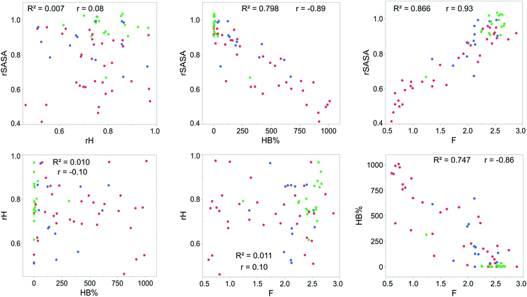
For each gelator–solvent combination, a 50 ns molecular dynamics simulation was performed to obtain a time averaged value for the descriptors (Fig. 3). All possible 2D plots between the four molecular descriptors (rSASA, HB%, rH and F) are presented in Fig. 4, together with their respective linear regression R² value and Pearson correlation coefficient (r). From these graphs, it can be seen that the molecular descriptors rSASA, HB% and F have an R² value between themselves ranging from 0.747 to 0.866. Additionally, their corresponding correlation coefficient is either higher than 0.85 or lower than −0.85 suggesting a linear trend between these descriptors. The negative linear trend between rSASA and HB% and between HB% and F might be expected. Indeed, as the gelator molecules in the simulation tend to aggregate in a solvent, the values of rSASA and F decrease as they quantify respectively the aggregation tendency and shape of the aggregate being formed by the gelator molecules. The HB%, on the other hand, will increase as more intermolecular hydrogen bonds are being formed between the gelator molecules in the aggregated state compared to the soluble state. With the same reasoning, the positive linear trend between rSASA and F can be rationalized. One might argue that because of the apparent linear relationship between rSASA, HB% and F, the aforementioned descriptors provide the same information and hence could be reduced to a single property. However, the following thought experiment demonstrates their unique intrinsic value and their independency from one another. Imagine a class of gelators consisting solely out of carbon and hydrogen atoms. The HB% descriptor will be equal to 0, regardless of the solvent and the gelator molecule as there are no hydrogen bond donor or acceptor atoms present. However, in this case rSASA and F will still vary upon changing the solvent as the solubility of the molecule and the aggregates shape of the aggregates can be influenced by other gelator–solvent interactions such as van der Waals interactions. In this case, no linear trend would be observed between HB% and rSASA or between HB% and F. Note, that this statement is supported by the 2-dimensional plots of rSASA vs. HB% and HB% vs. F in Fig. 4. In these plots, systems that are characterized by a value of HB% close to 0 still differ significantly in their values of rSASA (ranging from approximately 0.85 to 1.00) and F (ranging from approximately 2.00 to 3.00). Otherwise, the independency between rSASA and F can be demonstrated by imagining a set of gelator molecules that do not self-aggregate in a range of solvents. Here the rSASA will always be valued close to 1. Nevertheless, the value of F can still vary depending on the placement of the gelator molecules in the solvent. For example, a 1-dimensional alignment of the gelator molecules connected to each other through a solvent molecule will have a substantially larger value of F compared to a disperse placement of the gelator molecules, while both cases have an rSASA value close to 1. Although to a lesser extent, this is observable in the 2-dimensional plot of rSASA vs. F for values of rSASA close to 1. As such, while the descriptors rSASA, HB% and F might seem to be linearly correlated for the systems under investigation, they are independent from each other and provide their own unique information. rH shows no apparent linear trend with any of the molecular descriptors. This is because rH is highly dependent on the structure and flexibility of the gelator molecule and only mildly dependent on the aggregation behaviour. Compound 6, for example, has only two free rotatable bonds in its backbone, resulting in an rH value larger than 0.9, independent of the solvent. In contrast, compound 11 contains a large amount of rotatable bonds in its backbone, resulting in an rH value ranging from 0.55 to 0.78 (Table S2†). With this in mind, rH is a descriptor of the flexibility of the molecule under study.

Fig. 4 2D-scatter plots of the molecular descriptors proposed for predicting supramolecular gelation for the complete dataset. The points are coloured according to their outcome of the gelation test (S = green, G = blue and P = red). The Pearson correlation coefficient (r) and the coefficient of determination (R²) between two descriptors are provided as well.

When allocating the data points in the graph to the respective experimental result of the gelation test (green = soluble, blue = gel, red = precipitate), it is clear that soluble samples are characterized by a high value of rSASA and F and a low value of HB%, whereas a gel material is characterized by intermediate values of rSASA, F and HB%. Following this reasoning, samples resulting in a precipitate should be characterized by a low value of rSASA and F and a high value of HB% (Fig. 5). While a majority of the data agrees with this trend, there remain several outliers, especially when the sample forms a precipitate. For example, compound 8 in 1-octanol is experimentally classified as a precipitate (Table 1). Nevertheless, from the respective molecular dynamics simulations, relatively high values of rSASA (0.8818) and F (2.74) and a low value of HB% (162.40%) were obtained (Table S2†). This makes prediction of supramolecular gelation by visually inspecting the 2D-plots of the molecular descriptors challenging. However, we believe that the latter can be achieved by increasing the size of the simulation box, increasing the total simulation time and/or using more accurate sampling techniques such as ab initio molecular dynamics. At present, these methods would render the simulation computationally intractable.

Fig. 5 Representation of the general trend followed by the descriptors rSASA, F and HB% depending on the outcome of the gelation test. A snapshot of the MD simulation of 6 in DMSO (left, soluble), water (middle, gel) and heptane (right, precipitate) is given for illustrative purposes. The gelator molecules are visualized by a vdW representation and the solvent molecules by a tube representation. The solvent molecules are made transparent for clarity.

Prediction using machine learning methods

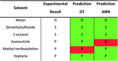
In recent years, several machine learning (ML) methods have established themselves in different areas of chemical research.³⁸ For example in targeted drug discovery, where ML can be used to model quantitative structure–activity relationships (QSAR).^39,40 Also in theoretical chemistry these methods have shown to assist the interpretation of complex calculations, replace otherwise computationally demanding methods, develop new accurate density functionals or force fields and even predict the electronic charge density and density of states within the framework of density functional theory (DFT).^41–45 Moreover, in the field of materials discovery, ML methods have shown their usefulness as evidenced by the earlier referred work of Gupta et al.^14,46,47 In this work, two separate ML methods, a decision tree and an artificial neural network (ANN), are used to showcase the ability to predict supramolecular gelation by the proposed molecular descriptors.⁴⁸ To achieve this challenging goal, the data is partitioned as follows: all data points coming from compound 11 will be used for testing, while the rest is used for training and validating the models (Table S3†). As such, the classification ability of the models will be tested on an unseen compound that can show any of the three responses (gel, soluble, precipitate) depending on the solvent. The models were constructed using JMP Pro version 14.⁴⁹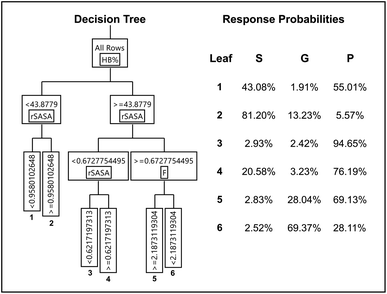

Decision tree. Decision trees (DT) are intuitive flowchart-like diagrams, where nodes create branches that partition the data based on a selected descriptor.⁴⁸ More nodes in the tree translate to a more branched, complex DT that has the tendency to produce an over fitted model. One of the major assets of DT over other machine learning methods is their transparent nature, making the prediction process easily understandable. The optimized DT model together with the response probabilities of each leaf is presented in Fig. 6. As is shown, the DT model contains five nodes resulting in a total of six leaves. The optimization procedure for the DT model is described in detail in the ESI (S20†). Upon closer investigation, leaf 2 shows the highest probability for the sample to be soluble (81.20%). When inspecting the flowchart, we can see that this leaf is characterized by a low value for HB% (<43.878) and a high value for rSASA (>0.958). Furthermore, leaf 3 is characterized by a high value for HB% (>43.877) and a low value for rSASA (<0.622) and shows the highest probability for a precipitate response (94.65%). This is in close agreement with our earlier observed trend for these descriptors (Fig. 5). The compound–solvent combination is predicted to be a gel if it is categorized in leaf 6, with the certainty of the prediction being 69.37%. This is considerably lower compared to the predictions made from leaf 2 and leaf 3 for soluble and precipitation respectively. A possible reason for this difference is most likely that cases where gelation is observed are rare in comparison to soluble and precipitated samples. Notably, the descriptor rH is never selected as a node in the optimized DT model. The node selection is based on the split that results in the statistically best performing model for the training data. Hence, this suggests that the rH descriptor does not provide the same predictive value in a partitioning model compared to the other three descriptors HB%, rSASA and F. Again, this is in line with our previous observations (Fig. 5).

Fig. 6 Diagram of the optimized decision tree having 5 nodes (left) and gelation outcome probability reported for the six resulting leaves (right).

A subset of 14 data points, which was randomly stratified according to the gelation response, was used as validation to assess the quality of the DT model and avoid over fitting. The remaining data was used for training (Table S3† specifies which data is used during training, validation and final testing). Multiple measures of fit, such as the balanced accuracy (BA), entropy R², the misclassification rate (MR), Cohen's kappa (K) and the area under the receiver operating characteristics curve for the three responses (AUROC (S), AUROC (G), AUROC (P)) are summarized for the training set (T), validation set (V) and a hypothetical perfect model (P) and random model (R) in Table 2. A definition for each of these statistical evaluation metrics is provided in the ESI (S23†). From Table 2, we observe that the DT model is adequately fitted as the training and validation data show similar values for all measures. Models that are over fitted are characterized by large discrepancies between the measures of fit obtained from training data and validation data (i.e. excellent measures of fit are obtained on the training set, but poor measures of fit are obtained on the validation set). Additionally, the DT exhibits substantial predictive behaviour, when comparing the measures of fit of the validation set to a perfect and random model.

Table 2 Performance statistics of the decision tree model for the training set (T) and validation set (V). For comparative reasons, the measures of fit for a hypothetical perfect model (P) and random model (R) are also provided

Measure	T	V	P	R
BA	0.72	0.68	1	0.33
Entropy R^2	0.50	0.48	1	0
MR	0.23	0.27	0	0.67
K	0.67	0.61	1	0
AUROC (S)	0.93	0.91	1	0.50
AUROC (G)	0.92	0.86	1	0.50
AUROC (P)	0.88	0.93	1	0.50

---

Artificial neural network. Artificial neural networks (ANN) are built out of a number of neurons, with each neuron accepting inputs, applying a weighted function to the inputs and forwarding the new information till eventually an output is reached.⁴⁸ The flexibility of ANN is evidenced by the myriad of hyperparameters that are adjustable, such as: the number of neurons, the transformation function used, number of hidden layers (if more than 3 hidden layers are used, the network is referred to as a deep neural network) and the method of optimizing the weight coefficients.^48,50 Due to this flexibility, highly accurate non-linear predictive models can be constructed. As such, in contrast to a decision tree, an ANN generally provides a less understandable “black box” predictive model. With this in mind, one needs to be extra wary for over fitting when architecting an ANN. This is usually accomplished by training and validating the model on hundreds to millions of data points. In this study, the amount of data is on the lower side of the spectrum. For this reason, two precautions were taken during the construction of the neural network to mitigate overfitting issues. First, the neural networks architecture is kept relatively simple, with a maximum of 5 neurons being considered during the hyperparameter optimization (S21†). As a neural network consists out of more neurons, the associated number of weights that need to be optimized during the training grows, which subsequently increases the complexity of the network and the possibility of overfitting. Second, a 5-fold cross validation was employed instead of a percentage holdback validation. In a 5-fold cross validation, or in general a k-fold cross validation, the data is randomly partitioned in 5 (or k) subsets. Next, for each set a neural network is trained with 4 sets as training data and the remaining set to validate the model. In total 5 different models are built with each set being used for validation once. Using this approach, data usage is maximized as all data points (of molecule 1–10) are employed during training equally. Importantly, signs of overfitting can be detected by discrepancies between the measures of fit obtained on the training and validation data.⁵¹ The optimized ANN (Fig. 7) is built out of 1 hidden layer that consists of 5 hyperbolic tangent neurons of which the weight coefficients are determined by a weight decay procedure (S21†). All measures of fit indicate that the ANN has excellent predictive abilities and outperforms the decision tree-based model (Table 3). Indeed, the measures of fit obtained on the training and validation data from the ANN model are closer to a hypothetical perfect model compared to the metrics obtained with the DT model. Most likely this can be explained by the superior flexibility of artificial neural networks over classical decision tree models.

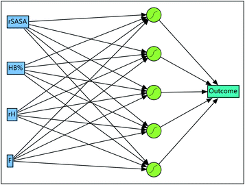Fig. 7 Optimized artificial neural network consisting out of the input layer, a hidden layer having 5 sigmoid neurons and the output layer.

Table 3 Performance statistics of the artificial neural network for the training set (T) and validation set (V). For comparative reasons, the measures of fit for a hypothetical perfect model (P) and random model (R) is provided

Measure	T	V	P	R
BA	0.97	1	1	0.33
Entropy R^2	0.82	0.93	1	0
MR	0.03	0	0	0.67
K	0.96	1	1	0
AUROC (S)	0.98	1	1	0.50
AUROC (G)	1	1	1	0.50
AUROC (P)	0.98	1	1	0.50

---

Predicting supramolecular gelation of an unknown urea-based molecule. As mentioned earlier, none of the data associated with the gelation ability of compound 11 in different solvents was used during the development of the decision tree and the artificial neural network. To test the predictive ability of both models on an unseen urea-based gelator, the DT and ANN models were applied to predict the outcome of the gelation tests of compound 11. Both models give satisfactory results, as 5 out of 6 cases for the gelation outcomes were predicted correctly (Table 4). Importantly, the two models successfully predicted that a supramolecular gel was formed in water. This confirms the ability of the proposed molecular descriptors to predict supramolecular gelation of urea-based compounds in a variety of solvents, with the prediction being a three-level classification of the sample being a solution, a precipitate or a gel.

Table 4 Experimental and predicted (decision tree DT and artificial neural network ANN) outcome of the gelation test of compound 11 in various solvents

---

Upon closer inspection of the gelator molecules that are present in the dataset, it can be observed that compound 6–11 have a more similar molecular structure compared to compound 1–5 (Fig. 2). Therefore, the quality of prediction of the gelation performance of compound 11 with models where compound 1–10 were used during training and validation, might be explained by the high resemblance of 11 with 6–10. To further investigate this, several neural networks were optimized, with the same architecture as the neural network described above, i.e. 1 hidden layer and 5 hyperbolic tangent neurons with the weight of each neuron optimized through a weight decay procedure. But in each neural network all data associated with a certain gelator molecule from the data set was subsequently left out during the training of the model and used for validation, similar to a leave-one-out cross validation approach. Validation statistics of each molecule separately together with the average measures of fit across molecules 1–10 are provided in Table 5. The results of this analysis establish that the models provide the best predictive qualities for compound 6–10, as the lowest observed entropy R² for these molecules is equal to 0.99 (compound 6). Nevertheless, substantial predictive power is also observed for compound 1–4, with the lowest observed entropy R² for this set being equal to 0.5 (compound 3). Only the model where compound 5 was left out for validation, shows significantly less predictive prowess with a misclassification rate of 0.20 and an entropy R² value of 0.09. All-in-all, the validation data on each molecule separately and the average measures of fit across the different neural networks indicate the ability of the descriptors to predict supramolecular gelation of an unknown compound. We should, however, highlight that 5 to 6 data points are associated with each gelator molecule and hence the validation statistics presented in Table 5 are taken over a low amount of data. Additionally, we want to acknowledge that both the decision tree and neural network models validate the predictive ability of the derived molecular descriptors over supramolecular gelation, however for practical purposes, these models would benefit greatly from a substantial increase in training data.

Table 5 Validation statistics obtained from a neural network with 1 hidden layer and 5 hyperbolic tangent neurons where sequentially compound 1–10 was left out for validation. Averages of the performance statistics are provided as well

Molecule	BA	Entropy R^2	MR	K	AUROC (S)	AUROC (G)	AUROC (P)
1	1	0.96	0	1	1	1	1
2	1	0.90	0	1	N.A.	1	1
3	1	0.50	0	1	1	1	N.A.
4	1	1	0	1	1	1	1
5	0.50	0.09	0.20	0.44	0.88	N.A.	0.88
6	1	0.99	0	1	1	1	1
7	1	1	0	1	1	N.A.	1
8	1	1	0	1	1	N.A.	1
9	1	1	0	1	1	N.A.	1
10	1	1	0	1	1	N.A.	1
Average	0.95	0.85	0.02	0.94	0.99	1	0.99

---

Outlook

While this work showcases that predicting supramolecular gelation based on descriptors derived from molecular dynamics simulations is feasible, there are still a number of factors limiting their applicability. Here, an overview of these factors is given and we discuss how they might be mitigated or overcome in the near future.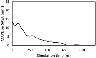

Robustness of descriptors. The four descriptors defined in this work: rSASA, rH, HB% and F are obtained through molecular dynamics simulations. Naturally, questions arise on the robustness and reproducibility of these descriptors as the results can be influenced by the total simulation time over which the descriptors are calculated, the initial topology of the simulation box and the randomness that is intrinsically related to molecular dynamics. The choice of the simulation time is determined by a balance between accuracy and computational workload. Longer simulations provide more accurate results but require more computer time. To ensure that a 50 ns would provide sufficient sampling to obtain trustworthy average values, a single 1 μs simulation was run for compound 6 in water. To make this simulation computationally tractable, the cubic simulation box edge was set at 40.32 Å and contained 5 gelator molecules and 2247 water molecules to reach a gelator concentration of 5.0% w/v. All other settings remained identical to the simulations that were performed to obtain the descriptors in this study. From the evolution of the average computed SASA during this simulation, the mean absolute percentage error (MAPE) on the average SASA obtained from a 50 ns is only 13% if the true average SASA is taken as the one obtained from the full μs simulation (Fig. 8). Hence, a total simulation time of 50 ns simulation can be regarded as adequate sampling, while still retaining sufficient computational speed. Especially if one considers that at 200 ns, which requires a computational workload that is 4 times higher as a 50 ns simulation, the MAPE still exceeds 5%.

Fig. 8 Evolution of the MAPE on the time averaged SASA during the simulation. The average SASA obtained after 1 microsecond is regarded as the true value.

To further increase the reproducibility of the computed values of the descriptors, initial topologies of the simulation were ensured to have the gelator molecules completely dispersed in the solvent, i.e. no atoms of the gelator molecules are closer than 3.0 Å from each other at the start of the simulation. To demonstrate the robustness of this method, simulations of compound 2, 5 and 6 in DMSO, ethanol and acetonitrile respectively, were performed in triplicate. From Table 6 it is concluded that this method provides highly repeatable values for each descriptor, as the deviation between the three simulations for each descriptor is relatively small for all systems that were considered. Especially when comparing the standard errors on the averages with the full range of values that were obtained in this study, the reliability of this method is shown.

Table 6 Computed values of rSASA, rH, HB% and F for 2 in DMSO, 5 in ethanol and 6 in acetonitrile performed in triplicate. Average values including the standard error are provided as well as the approximate range of values that were calculated for each descriptor in this study (between square brackets)

System	Entry	rSASA [0.4–1.0]	rH [0.5–1.0]	HB% [0–1010]	F [0.6–2.9]
Compound 2 in DMSO	1	0.958	0.510	0.030	2.1
	2	0.965	0.526	0.020	2.8
	3	0.963	0.535	0.000	2.7
	Average	0.962 ± 0.004	0.524 ± 0.013	0.017 ± 0.015	2.6 ± 0.4
Compound 5 in ethanol	1	0.933	0.790	2	2.26
	2	0.928	0.787	8	2.55
	3	0.927	0.786	7	2.54
	Average	0.929 ± 0.003	0.788 ± 0.002	6 ± 3	2.45 ± 0.16
Compound 6 in acetonitrile	1	0.912	0.970	73	2.5
	2	0.922	0.969	74	2.8
	3	0.907	0.970	104	2.9
	Average	0.913 ± 0.007	0.9698 ± 0.0007	84 ± 18	2.7 ± 0.2

---

Computational limitations. As the descriptors originate from a molecular dynamics simulation, their usefulness is highly dependent on how accurate the real system is modelled. As briefly mentioned above, simulating bigger systems (i.e. more gelator and solvent molecules) for a longer time (i.e. more timesteps) might increase the predictive potential. Furthermore, as computing power is constantly improving, the level of theory employed to run the simulations can become more accurate as well, enhancing the merits of the descriptors even further.⁵² Next, it is also important to note that if one would want to apply this method to discover a new LMWG, a screening of hundreds to thousands of compounds might be necessary. This level of throughput is at present not computationally viable at an all-atom scale. The latter can become possible, however, by software benefiting from state-of-the art technologies and hardware.^53,54

Applicability domain. It is important to delineate the boundaries of the applicability domain of the predictive methods proposed in this work.⁵⁵ While the focus was to predict supramolecular gelation of simple organic urea-based molecules, these boundaries are still somewhat ambiguous. If certain types of atoms or functional groups are not well represented during the training of the predictive model, cases for which the LMWG contains such a functional group might fall outside the applicability domain, even if the LMWG is a urea-based molecule. For traditional QSAR models, various methods exist to determine the applicability domain, such as a Principle Component Analysis (PCA), distance to model (DM) or a K Nearest Neighbours (KNN) approach.^56–58 These methods are, however, ineffective in this case due to the relatively low number of descriptors and data points. One way to mitigate this problem, is to scan the applicability boundary by calculating the descriptors and implementing a similar method to predict other classes of materials, such as peptide or glycosylated supramolecular gels. Additionally, we underline that the models only predict supramolecular gelation based on a specific gelation procedure and minimum gelation concentration. This is important because some molecule–solvent combinations might be classified as a non-gel by the model, while a different gelation trigger or concentration does render them a gel. For example, compound 8 in water is known to form a gel by introducing sonication during the gelation procedure.¹⁷ However, here it is classified as a precipitate because the gelation procedure, on which the model is based, only uses heating and subsequent cooling as a trigger. In principle, for every different gelation procedure a new predictive model should be built requiring a library of data points obtained following exactly the same protocol for gelation performance.

Prediction of material properties. The material properties largely determine the usefulness of a supramolecular gel in certain applications. For example, in drug delivery and 3D bio-printing where the material needs to retain or recover their gel state upon injection. It would be interesting to see if descriptors, similar as proposed in this work, could be used to make a prediction regarding relevant properties such as the yield strain, storage modulus or loss modulus. To achieve this, a uniform dataset containing these properties of several supramolecular gels needs to be gathered, which will be the scope of future works.

Conclusion

Predicting supramolecular gelation on the basis of computations is regarded as a challenging task. In this study, four molecular dynamic based descriptors with physical relevance to supramolecular gelation are introduced: the relative solvent accessible surface area (rSASA) to evaluate aggregation, the relative end-to-end distance (rH) describing the flexibility and conformational preferences of the molecules, the hydrogen bonding percentage (HB%) to quantify the non-covalent linkage of the gelator molecules, and the shape factor (F) which is a measure for the aggregate's shape. Via two separate machine learning techniques, it was demonstrated that these descriptors can accurately differentiate the gelation response of a set of urea-based gelators as a precipitate, a gel or a fully solubilised sample. To the best of our knowledge, this is the first computational method that addresses the prediction of urea-based supramolecular gelation in both organic solvents as well as in water. We hope that the proposed descriptors can be conceptualized for other types of gelators and will steer the field to discover potential new low molecular weight gelators in the near future.

Conflicts of interest

There are no conflicts to declare.

Acknowledgements

Tier2 computational resources and services were provided by the Shared ICT Services Centre Funded by the Vrije Universiteit Brussel, the Flemish Supercomputer Center (VSC) and FWO. The Strategic Research Program funding of the VUB is thanked for financial support. F. D. P. also acknowledges the Francqui foundation for a position as “Francqui research professor”. R. V. L. thanks FWO for the PhD fellowship received (1185219N) and Jos L. Teunissen for valuable discussions. M. A. thanks the FWO for a postdoctoral fellowship (12F4416N) and the VUB for financial support.

Notes and references

1. K. J. Skilling, F. Citossi, T. D. Bradshaw, M. Ashford, B. Kellam and M. Marlow, Soft Matter, 2014, 10, 237–256.
2. B. Escuder, F. Rodríguez-Llansola and J. F. Miravet, New J. Chem., 2010, 34, 1044–1054.
3. S. Ghosh, V. K. Praveen and A. Ajayaghosh, Annu. Rev. Mater. Res., 2016, 46, 235–262.
4. E. R. Draper and D. J. Adams, Chem, 2017, 3, 390–410.
5. P. Dastidar, Chem. Soc. Rev., 2008, 37, 2699–2715.
6. A. R. Hirst, I. A. Coates, T. R. Boucheteau, J. F. Miravet, B. Escuder, V. Castelletto, I. W. Hamley and D. K. Smith, J. Am. Chem. Soc., 2008, 130, 9113–9121.
7. R. Van Lommel, L. A. J. Rutgeerts, W. M. De Borggraeve, F. De Proft and M. Alonso, ChemPlusChem, 2020, 85, 267–276.
8. M. Raynal and L. Bouteiller, Chem. Commun., 2011, 47, 8271–8273.
9. J. Bonnet, G. Suissa, M. Raynal and L. Bouteiller, Soft Matter, 2015, 11, 2308–2312.
10. D. Rosa Nunes, M. Raynal, B. Isare, P.-A. Albouy and L. Bouteiller, Soft Matter, 2018, 14, 4805–4809.
11. P. Frederix, G. G. Scott, Y. M. Abul-Haija, D. Kalafatovic, C. G. Pappas, N. Javid, N. T. Hunt, R. V. Ulijn and T. Tuttle, Nat. Chem., 2015, 7, 30–37.
12. I. P. Moreira, G. G. Scott, R. V. Ulijn and T. Tuttle, Mol. Phys., 2019, 117, 1151–1163.
13. P. W. J. M. Frederix, R. V. Ulijn, N. T. Hunt and T. Tuttle, J. Phys. Chem. Lett., 2011, 2, 2380–2384.
14. J. K. Gupta, D. J. Adams and N. G. Berry, Chem. Sci., 2016, 7, 4713–4719.
15. D. J. Adams and P. D. Topham, Soft Matter, 2010, 6, 3707–3721.
16. E. Ye, P. L. Chee, A. Prasad, X. Fang, C. Owh, V. J. J. Yeo and X. J. Loh, Mater. Today, 2014, 17, 194–202.
17. L. A. J. Rutgeerts, A. H. Soultan, R. Subramani, B. Toprakhisar, H. Ramon, M. C. Paderes, W. M. De Borggraeve and J. Patterson, Chem. Commun., 2019, 55, 7323–7326.
18. K. Yabuuchi, E. Marfo-Owusu and T. Kato, Org. Biomol. Chem., 2003, 1, 3464–3469.
19. N. Zweep, A. Hopkinson, A. Meetsma, W. R. Browne, B. L. Feringa and J. H. van Esch, Langmuir, 2009, 25, 8802–8809.
20. M. George, G. Tan, V. T. John and R. G. Weiss, Chem.–Eur. J., 2005, 11, 3243–3254.
21. A. E. Hooper, S. R. Kennedy, C. D. Jones and J. W. Steed, Chem. Commun., 2016, 52, 198–201.
22. Y. Sang and M. Liu, Mol. Syst. Des. Eng., 2019, 4, 11–28.
23. C. Fang, M. Fantin, X. Pan, K. de Fiebre, M. L. Coote, K. Matyjaszewski and P. Liu, J. Am. Chem. Soc., 2019, 141, 7486–7497.
24. S. G. Robinson, Y. Yan, K. H. Hendriks, M. S. Sanford and M. S. Sigman, J. Am. Chem. Soc., 2019, 141, 10171–10176.
25. N. Foloppe and J. A. D. MacKerell, J. Comput. Chem., 2000, 21, 86–104.
26. V. Zoete, M. A. Cuendet, A. Grosdidier and O. Michielin, J. Comput. Chem., 2011, 32, 2359–2368.
27. M. H. Mamme, S. L. C. Moors, E. A. Mernissi Cherigui, H. Terryn, J. Deconinck, J. Ustarroz and F. De Proft, Nanoscale Adv., 2019, 1, 2847–2856.
28. M. Parrinello and A. Rahman, J. Appl. Phys., 1981, 52, 7182–7190.
29. M. J. Abraham, T. Murtola, R. Schulz, S. Páll, J. C. Smith, B. Hess and E. Lindahl, SoftwareX, 2015, 1–2, 19–25.
30. L. Martinez, R. Andrade, E. G. Birgin and J. M. Martinez, J. Comput. Chem., 2009, 30, 2157–2164.
31. J. H. van Esch, Langmuir, 2009, 25, 8392–8394.
32. F. Eisenhaber, P. Lijnzaad, P. Argos, C. Sander and M. Scharf, J. Comput. Chem., 1995, 16, 273–284.
33. J. van Esch, F. Schoonbeek, M. de Loos, H. Kooijman, A. L. Spek, R. M. Kellogg and B. L. Feringa, Chem.–Eur. J., 1999, 5, 937–950.
34. P. Byrne, D. R. Turner, G. O. Lloyd, N. Clarke and J. W. Steed, Cryst. Growth Des., 2008, 8, 3335–3344.
35. K. Pandurangan, J. A. Kitchen, S. Blasco, F. Paradisi and T. Gunnlaugsson, Chem. Commun., 2014, 50, 10819–10822.
36. R. B. Best, G. Hummer and W. A. Eaton, Proc. Natl. Acad. Sci. U. S. A., 2013, 110, 17874.
37. W. Burchard, Light Scattering from Polymers, Springer Berlin, Heidelberg, Berlin, Heidelberg, 1983, pp. 1–124.
38. K. T. Butler, D. W. Davies, H. Cartwright, O. Isayev and A. Walsh, Nature, 2018, 559, 547–555.
39. Y.-C. Lo, S. E. Rensi, W. Torng and R. B. Altman, Drug Discovery Today, 2018, 23, 1538–1546.
40. X. Yang, Y. Wang, R. Byrne, G. Schneider and S. Yang, Chem. Rev., 2019, 119, 10520–10595.
41. F. Häse, I. F. Galván, A. Aspuru-Guzik, R. Lindh and M. Vacher, Chem. Sci., 2019, 10, 2298–2307.
42. J. C. Snyder, M. Rupp, K. Hansen, K.-R. Müller and K. Burke, Phys. Rev. Lett., 2012, 108, 253002.
43. V. Botu, R. Batra, J. Chapman and R. Ramprasad, J. Phys. Chem. C, 2017, 121, 511–522.
44. A. Chandrasekaran, D. Kamal, R. Batra, C. Kim, L. Chen and R. Ramprasad, npj Comput. Mater., 2019, 5, 22.
45. O. A. von Lilienfeld, Angew. Chem., Int. Ed., 2018, 57, 4164–4169.
46. Y. Liu, T. Zhao, W. Ju and S. Shi, J. Materiomics, 2017, 3, 159–177.
47. A. Mansouri Tehrani, A. O. Oliynyk, M. Parry, Z. Rizvi, S. Couper, F. Lin, L. Miyagi, T. D. Sparks and J. Brgoch, J. Am. Chem. Soc., 2018, 140, 9844–9853.
48. E. Alpaydin, Introduction to Machine Learning, MIT Press, Cambridge, 2010.
49. JMP®, Version Pro 14, SAS Institute Inc., Cary, NC, 1989–2019.
50. G. B. Goh, N. O. Hodas and A. Vishnu, J. Comput. Chem., 2017, 38, 1291–1307.
51. Classically, in a k-fold cross validation the data set is randomly divided into k-subsets. Next, for each subset a model is made where the k^th subset is used for validation and the rest of the data as training data. As such k models are built. The validation performance statistics are then determined by averaging over the k models. In the JMP software, however, the model that shows the best performance for a certain fold k is chosen as the final model upon which the validation metrics are based.
52. S. Grimme and P. R. Schreiner, Angew. Chem., Int. Ed., 2018, 57, 4170–4176.
53. C. Kutzner, S. Páll, M. Fechner, A. Esztermann, B. L. de Groot and H. Grubmüller, J. Comput. Chem., 2019, 40, 2418–2431.
54. K. Sugisaki, S. Nakazawa, K. Toyota, K. Sato, D. Shiomi and T. Takui, ACS Cent. Sci., 2019, 5, 167–175.
55. A. Tropsha, Mol. Inf., 2010, 29, 476–488.
56. J. Jaworska, N. Nikolova-Jeliazkova and T. Aldenberg, Altern. Lab. Anim., 2005, 33, 445–459.
57. R. P. Sheridan, B. P. Feuston, V. N. Maiorov and S. K. Kearsley, J. Chem. Inf. Comput. Sci., 2004, 44, 1912–1928.
58. I. Sushko, S. Novotarskyi, R. Körner, A. K. Pandey, V. V. Kovalishyn, V. V. Prokopenko and I. V. Tetko, J. Chemom., 2010, 24, 202–208.

---

Footnote

† Electronic supplementary information (ESI) available. See DOI: 10.1039/d0sc00129e

---