Grafting metal complexes onto amorphous supports: from elementary steps to catalyst site populations via kernel regression

Abstract

Ab initio computational studies have made tremendous progress in describing the behavior of molecular (homogeneous) catalysts and crystalline versions of heterogeneous catalysts, but not for amorphous heterogeneous catalysts. Even widely used industrial amorphous catalysts like atomically dispersed Cr on silica remain poorly understood and largely intractable to computational investigation. The central problems are that (i) the amorphous support presents an unknown quenched disordered structure, (ii) metal atoms attach to various surface grafting sites with different rates, and (iii) the resulting grafted sites have different activation and catalytic reaction kinetics. This study combines kernel regression and importance sampling techniques to efficiently model grafting of metal ions onto a non-uniform ensemble of support environments. Our analysis uses a simple model of the quenched disordered support environment, grafting chemistry, and catalytic activity of the resulting grafted sites.

---

1. Introduction

Most ab initio computational catalysis studies focus on homogeneous catalysts,^1–3 enzymes,^4–6 or heterogeneous catalysts with ordered structures such as metals,^7–11 zeolites,^12–14 and crystalline metal oxides.^15–17 All of these materials have in common the advantage that many features of the catalyst structure are known. Even for molecular catalysts and enzymes, where the active site resides within a fluctuating environment, there are systematic computational frameworks for averaging over the fluctuations.^18–20 In contrast, amorphous catalysts cannot be modelled with small, periodically repeating solid structures, nor by sampling a well-defined ensemble for liquid phase disorder. Instead, the quenched disorder in an amorphous heterogeneous catalyst^21,22 is a permanent signature of its non-equilibrium preparation history. Examples within this family include the Phillips catalyst (Cr/SiO₂) for ethylene polymerization,²³ molybdenum (Mo/SiO₂) and tungsten (W/SiO₂) catalysts for olefin metathesis,²⁴ and titanium catalysts (Ti/SiO₂) for alkene epoxidation.²⁵

Because of these difficulties, amorphous catalysts have mostly been avoided in ab initio computational studies. Those exceptions in which calculations on amorphous catalysts were attempted were forced to rely on questionable assumptions.^22,26–34 For example, are the model sites representative of the real material? Do the models accurately represent the most active sites? Can reliable conclusions about the reaction kinetics be drawn from a single-site computational model? At present, none of these questions can be satisfactorily answered with ab initio calculations.

These questions are addressed in two papers, this one and a companion. They provide a computational framework that combines machine learning, statistical importance sampling, and population balance modeling techniques. To illustrate the concepts and methods, we begin with a model for an atomically-dispersed catalyst on an amorphous support. The essential features of the model are a quenched disordered support scaffold (to represent an amorphous silica matrix), surface silanol sites where precursors can be attached (to represent surface hydroxyl groups), and a microkinetic model for grafting at each silanol site. These microkinetic models have rate parameters that depend on the individual grafting site characteristics. The rate parameters at each grafting site will be determined, much like in a real ab initio calculation, by structural optimization of the intermediates using a simple force field.

This first paper deals with how the active sites are generated during catalyst preparation. In particular, we show how the populations of both grafted sites and the unreacted grafting sites evolve during an idealized grafting process. If the surface reactions are irreversible, the final metal site distribution will be determined by those surface grafting sites with the fastest grafting kinetics. However, if the surface reactions are reversible, the final grafted site distribution will favor grafted sites that lead to the most stable grafted species. To enable ab initio studies in the future, the algorithm must efficiently predict the characteristics of the most reactive grafting sites and their abundances, without performing exhaustive ab initio calculations for many thousands of grafting sites. We demonstrate how kernel regression can learn to anticipate the outcomes of these optimizations. Then, by applying the kernel regression model to thousands of grafting sites, we can construct a population balance model for the grafting process. The simplicity of our model system allows us to test the accelerated predictions against an exhaustive parameterization from structure optimizations at thousands of grafting sites.

The companion paper uses a grafted site population that reflects both the disordered support and the superimposed grafting kinetics to predict site-averaged kinetics. Because turnover frequencies at individual grafting sites depend exponentially on their activation energies, site-averaged kinetics are difficult to converge without rare events sampling methods. The second paper deals with averaging over the non-uniform distribution of grafted sites to predict the overall kinetics.

The remainder of this paper is as follows. First, we introduce simple models for the amorphous support and grafting kinetics. Next, we use kernel regression tools to predict the grafting thermodynamics and kinetics based on a concise list of grafting site characteristics. Finally, we use the kernel regression results and kinetic models to parameterize the population balance model for grafting.

2. Amorphous silica

Amorphous silica is a commonly used catalyst support because of its thermal and mechanical stability, large surface area, and its chemical inertness. The surface of silica is terminated by silanol groups which may be categorized as isolated, geminal, vicinal etc. Real amorphous silicas are created via sol–gel synthesis, spray drying, pyrolysis, or precipitation methods. Silica can be calcined to increase its mechanical strength and to remove adsorbed water.^35–40 The calcination temperature also determines the residual surface silanol density, which in turn influences the activity of the supported catalyst.^23,41,42

Many studies have used spectroscopic techniques like IR, NMR, and EPR to investigate the populations of different silanol types.^43,44 However, in contrast to crystalline materials, the absence of long-range order results in broad peaks that complicate the precise characterization of silica.

Silicas of different types exhibit different ring size distributions,^45–47 and silanols of the same type can have different bond angles and different dihedral angles.^35,44 These subtle structural differences between silanols and their environments are likely to influence their reactivity. Many investigators have grafted metal atoms to silica via reactions between silanols and molecular complexes like AlCl₃,⁴⁸ GaR₃,^49,50 TiCl₄,^51–53 and VOCl₃.^54,55 These grafting reactions are useful both as probes of local structure and as routes to supported organometallic catalysts.

In a typical grafting experiment, a fluid phase molecular precursor reacts with amorphous silica.^49,55,56 A protonolysis reaction between the precursor and surface silanols results in a metal atom grafted to the silica surface with one, two, or three M–O–Si linkages, sometimes called monopodal, bipodal, or tripodal species, Fig. 1.^24,57–60

Fig. 1 Scheme showing the grafting of a molecular ML₂ complex to a vicinal silanol pair. The metal forms two bonds to the silanolate oxygens while two HL molecules are eliminated. The metal may also coordinate to nearby siloxane oxygens.

Computational studies of atomically-dispersed metals on silica often use cluster models terminated by hydroxyl groups or hydrogen atoms. These models generally range in sizes from a few to tens of silicon atoms.^{28,30,34,61–67} The cluster models are often carved from crystalline materials like zeolites⁶⁸ or β-cristobalite.^66,69 In such clusters, the peripheral atoms are fixed at positions characteristic of the crystalline material. The de facto assumption is that larger cluster models are more representative of the real amorphous catalyst. Indeed large cluster models more accurately account for elasticity of the silica matrix and for dispersion interactions between adsorbates and the support.^33,70 However, each layer of silica requires additional and unjustified assumptions about the environment. In this sense, large cluster models are overly specific, while small cluster models are amenable to systematic investigation of the effects of local grafting site geometry.²²

In the past decade, some computational studies generated amorphous silica surfaces that attempt to reproduce experimental observables like surface silanol density and the IR spectrum.^71–74 Typically, such surfaces are prepared by molecular dynamics simulations, in which crystalline models are heated to high temperatures followed by rapid quenching to generate disordered structures. Then the bulk amorphous structure is cleaved to create the surface. Unsaturated oxygens are capped with hydrogen atoms, and unsaturated silicons are capped with hydroxyl groups. Finally, pairs of proximal silanols are condensed to achieve the correct surface silanol density. These methods generate atomistic amorphous models of silica with a non-uniform structural distribution of surface silanols. However, such in silico preparation routes for amorphous silica do not correspond to experimental synthesis procedures. In particular, the high surface area of a real silica does not result from cleavage and subsequent functionalization. In addition, the system sizes modelled are typically quite small (100–200 silanols). For comparison, a 10 mg sample of silica with area 350 m² g⁻¹ and 1.0 silanols per nm² contains about 10¹⁸ silanols.

2.1. A simple model for amorphous silica

The mechanisms of grafting, activation, and catalytic reactions are still debated for many amorphous catalysts.^{26,30,50,58,69,75–77} To resolve the outstanding questions, we need methods that can predict the kinetics at each grafting site and estimate proper site-averaged kinetic properties. Then a given support model (if large enough) and proposed mechanism will yield well-defined, site-averaged predictions to be tested against experiments. To develop such methods, we selected a simple example system for which benchmark calculations can be performed exhaustively, for the full ensemble of non-uniform sites. In this section, we propose a simple abstract model of the amorphous support.

We model the amorphous support as a 2D lattice with quenched disorder, Fig. 2. Note the loose similarity to the qualitative model of Peri and Hensley.⁴⁸ First, a uniform lattice is created in which nearest neighbours are separated by a unit (dimensionless) distance. Each site is randomly displaced (δ) from the uniform lattice by random displacements along the x and y directions to create a disordered lattice. Displacements are drawn from an isotropic 2-D Gaussian distribution (described in the ESI†). The lattice is then “functionalized” with hydroxyl (–OH), siloxane (≡SiOSi≡), and empty sites with probabilities p_OH,p_siloxane, and p_empty.

Fig. 2 Steps to form a functionalized, quenched disorder lattice.

2.2. Grafting molecular metal complexes: a simple model

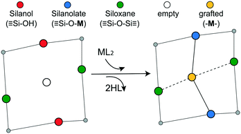
Grafting sites in our model are empty sites surrounded by a pair of vicinal hydroxyls on one axis and a pair of siloxanes on the other axis. Fig. 3 shows a grafting site located between vicinal silanols (≡SiOH)₂ and two siloxanes (≡SiOSi≡). The precursor ML₂, a molecular complex, in our model has two displaceable ligands. A real catalyst precursor may have additional ligands like chloride, oxo, or methyl groups that remain bonded to the metal M after grafting. The metal is grafted as a bipodal species (≡SiOMOSi≡) upon reaction of ML₂ with the vicinal hydroxyls to eliminate two HL molecules. The metal may also interact with neighbouring siloxanes to form M⋯O(Si≡)₂ bonds. The strengths of the ≡SiO–M and M⋯O(Si≡)₂ bonds depend on the local geometry near the grafting site.

Fig. 3 Grafting sites on the amorphous 2-D lattice model. One set of opposite nearest neighbour sites are hydroxyl groups, while the other set is siloxanes. ML₂ reacts with two hydroxyls and interacts with the siloxanes to create a grafted M atom as shown.

2.3. Computing grafting rates on the amorphous silica model

To model grafting kinetics of vicinal silanol sites on the amorphous 2D lattice, we consider the grafting mechanism outlined in sec. 2.2. The grafting process at each vicinal silanol site is assumed to be irreversible with the following rate law:

r(x) = k(x)[ML₂]. (1)

Here [ML₂] is the gas phase concentration of ML₂, x represents the local environment of the vicinal silanol site, and k(x) is a site-dependent rate constant.⁷⁸ We use concentration to construct rate laws in this work. One can instead use the precursor partial pressure, but note that one must beware of the resulting complications in extracting activation energies. For example, when precursor pressure is set by its T-dependent vapor pressure, as in CrO₂Cl₂ grafting,⁵⁸ the pressure and temperature cannot be separately controlled. We use transition state theory (TST) to model the temperature and site-geometry dependence of the grafting rate constant. TST rate constants are widely used to predict and interpret activation barriers and kinetics across a wide range of catalysis applications.^79–83 TST rate constants are now readily computed from electronic structure calculations.⁸⁴ The TST rate constant is:Here ΔG^‡(x) is the grafting barrier as computed with [ML₂] at the reference volume (V̂₀) per particle.

Next, we use a linear free energy relationship (LFER) to model the grafting free energy barrier. Specifically, we assume that the free energy of grafting is linearly related to the activation barrier for grafting:⁷⁸

Here α (0 < α < 1) is the Brønsted coefficient and is the grafting barrier for a reference grafting site with a thermoneutral grafting free energy (ΔG° = 0). The value of α indicates the position of the transition state between the reactant and product states. Small values of α (near 0) indicate an early transition state that resembles the reactants. Large values of α (near 1) indicate a transition state that resembles the products. In practice, intermediate values of α are common, so we have chosen α = 1/2.⁸⁵ The value of determines the time scale for grafting, but it will have no bearing on results after non-dimensionalization. Thus, to complete the kinetic model, including the effects of non-uniform grafting sites, we only need a model for ΔG°(x). The energy to graft the precursor at an empty site is

ΔE(x) = 2ε_HL + V_M*(x) − V_* − 2ε_ML. (4)

Here V_M*(x) is the energy of the grafted metal site, V_* is the energy of the unreacted silica site, ε_ML is the energy of the M–L bond, and ε_HL is the energy of the H–L bond. V_* is twice the O–H bond energy,

V_* = 2ε_OH. (5)

Here ε_OH is the O–H bond energy. To compute V_M*(x), the M–OSi≡ bond energy and M⋯O(Si≡)₂ bond energy are modelled as Morse potentials:

ε_i(r) = D_i(1 − exp[−a_i(r − r_i,eq)])² − D_i. (6)

Here i is the interaction type (M–OSi≡ or M⋯O(Si≡)₂), D_i is the equilibrium energy of the interaction, a_i is related to the width of the potential well, r_i,eq is the equilibrium distance, and r is the metal–oxygen bond length. All constants defined in this section are shown in Table 1. 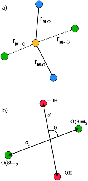V_M*(x) is computed by optimizing the position of the metal with surrounding hydroxyl and siloxane positions fixed:Here, r_M–Oi is a metal–oxygen bond distance, and is a metal–siloxane coordination distance, as shown in Fig. 4a. The bond lengths are functions of the (variable) metal atom position x_M and the (quenched/fixed) peripheral siloxane and silanol locations in x. The optimization indicated in eqn (7) therefore involves optimization of the metal atom position within the fixed peripheral environment.

Table 1 Constants used in computing grafting barriers and defining the quenched disorder lattice (see ESI for further explanations)

Parameter	Value
T	298.15 K
r M–O, eq	1.0
r M⋯O, eq	1.16
σ lattice ^2	0.00022
p OH	0.3
p siloxane	0.3
p empty	0.4
D M–O	524.4 kJ mol^−1
a M–O	1.9
D M⋯O	120 kJ mol^−1
a M⋯O	2.3
2εHL − (V* + 2εML) + ΔPV + ΔS°	1229.56 kJ mol^−1
M	0.026
α	0.5
	−30 kJ mol^−1
	131.3 kJ mol^−1

---

Finally, the free energy of grafting is computed using

ΔG°(x) = ΔE(x) + ΔPV − TΔS°. (8)

Here ΔS° is the entropy of the grafting reaction and ΔE(x) + ΔPV is the enthalpy. The entropy changes are predominantly from site-independent contributions like translational and rotational degrees of freedom of the ML₂ and HL species. As noted for the parameter , the site-independent terms in eqn (8) have no bearing on the results after non-dimensionalization.

Fig. 4 (a) Bond lengths in the force field and in the optimization of the M-atom position. (b) Coordinates for describing the local environment around the grafting site. We have used three of the five (2 × 4 – 1 (rotation) – 2 (translations)) peripheral environment coordinates in the initial kernel regression model.

3. Kernel regression model for grafting barriers

Because ab initio calculations are costly, computational studies of catalyst grafting have been based on single sites, or at most a few sites. Ultimately, one hopes to make predictions about grafting across the entire distribution of non-uniform sites. In this section, we propose a machine learning method (kernel regression) to learn structure–property relations from a modest number of training calculations.^86–88 Kernel regression was chosen because it is a non-parametric method; hence it does not need a predefined form for the fitting function. Specifically, we will use calculations at a small collection of grafting sites to predict barriers and kinetics for all grafting sites.

The training data includes a collection of computed barriers, ΔG^‡(x₁), ΔG^‡(x₂), ΔG^‡(x₃), etc. The estimated barrier for a new peripheral environment x is a kernel-weighted average of the training data:

Here, ΔĜ^‡(x) is the prediction for a grafting site with local geometry x, ΔG^‡(x_i) values represent the barriers of grafting sites in the training set, N_train is the number of training examples, and w(x, x_i) are the weights. The weights are represented using a Gaussian kernel:⁸⁹Here d²(x, x′) is a squared non-Euclidean Mahalanobis distance between structures x and x′

d²(x, x′) = (x − x′)^TS(x − x′). (11)

S is a square, symmetric, and positive definite matrix. To ensure that S remains positive definite while being optimized/learned, we write S as

S = AA^T. (12)

Here A is a lower triangular matrix.⁹⁰ Matrix A should be optimized so that eqn (9) accurately predicts ΔG^‡(x) at new grafting sites.

The training data from optimization of a small collection of grafting sites is used in a leave-one-out objective function

to determine A. In L, ΔĜ^‡(x_i) is a weighted average of all data points in the training set excluding itself:The Gaussian kernel in eqn (10) generates a continuous and differentiable model of ΔG^‡(x), so the leave-one-out error function is easily minimized with conjugate gradient methods or other superlinear minimization schemes.⁹¹ We use kernel regression as implemented in the metric-learn Python library.⁹² The library minimizes L using the conjugate gradient method with analytical derivatives of L.

4. Local coordinates

The Gaussian kernel function in eqn (9) can be constructed from the complete set of internal coordinates for the local environment. However, a subset of the internal coordinates will usually be sufficient to predict the activation barriers. We do not know a priori which coordinates are most important, but these can be identified as illustrated below.

The local environment of silanol and siloxane groups in our model is specified by five coordinates (2 dimensions × 4 “atoms” – 1 rotation – 2 centre-of-mass translations). We use three of the five coordinates to construct the kernel regression model: (1) distance between OH groups (d₁), (2) distance between siloxane groups (d₂), and (3) angle between the OH-siloxane groups (θ), Fig. 4.

5. Sites with non-uniform grafting barriers: a population balance perspective

As described in sec. 2., an amorphous support will have a distribution of grafting sites with different grafting rates. As time progresses, the most reactive grafting sites will be consumed, while grafting sites with higher reaction barriers remain unreacted and reduce the rate of further grafting. This situation can be modelled using the following population balance scheme:Here ρ(ΔG^‡, t) is the population of unreacted vicinal silanol sites at time t with a barrier of ΔG^‡,
is the rate at which the sites react (eqn (1)), and m = [ML₂]/V̂₀⁻¹ is the ratio of the concentration of the precursor ML₂ in the gas phase to the reference concentration (V̂₀⁻¹) at which ΔG^‡ is computed. The rate of change of m isHere, the first term on the right-hand side is rate of consumption of ML₂ due to the grafting reaction, and m_G is the rate at which ML₂ is fed to the reactor. In some grafting experiments, the molecular complex is constantly replenished by evaporation from a reservoir, so that its gas phase concentration is always in equilibrium with its liquid reservoir.^50,58 In such cases, the ML₂ concentration remains constant at its vapor pressure as grafting proceeds. Assuming constant m, eqn (15) can be integrated to yieldHere ρ₀(ΔG^‡) is the initial population of vicinal silanol sites.

Defining non-dimensional time as:

leads to the population of unreacted vicinal silanol sites as a function of τ and grafting free energy barrier:

ρ(ΔG^‡, τ) = ρ₀(ΔG^‡)exp[−e^−βαΔG°mτ]. (19)

6. Results and discussion

6.1. Evolution of grafting site population

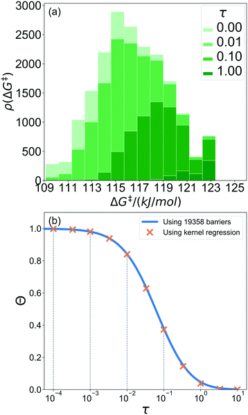
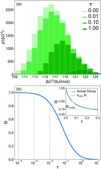
A 1500 × 1500 lattice was randomly perturbed using the procedure outlined in sec. 2.1. A total of 19 368 grafting sites were identified. A metal atom was placed in each grafting site, and its position was optimized. The grafting free energy barrier was computed for each grafting site. A histogram of the results was constructed to approximate the initial distribution ρ₀(ΔG^‡). Note that the horizontal axis depends on the choice of and ΔS°/k_B, i.e., different values of these parameters will shift the distribution left and right along the ΔG^‡ axis. In a real system, ab initio calculations yield ΔG^‡ and ΔS° values for all grafting sites with no adjustable parameters, so there would be no arbitrary shift. Following this, eqn (19) was used to compute the evolution of the unreacted grafting site population, Fig. 5a.

Fig. 5 (a) Evolution of the unreacted vicinal silanol site population as a function of non-dimensional grafting time. (b) Fraction of unreacted vicinal silanol sites as a function of logarithmic time. The inset shows the evolution as a function of real time in the range 0 < τ < 0.3. It also includes an exponential decay model fit to this data.

The initial range of grafting barriers spans 23 kJ mol⁻¹. Grafting sites with the lowest barriers react first, so the distribution shifts to the right as grafting proceeds. The 23 kJ mol⁻¹ width of the distribution causes the grafting sites to react at markedly different rates. The fastest grafting sites react in about 10⁻⁴τ. Grafting is complete in about 10 τ.

During a grafting experiment, the total number of grafted sites at any time can be measured, e.g., by monitoring the amount of HL released. The fraction of unreacted vicinal silanol sites (relative to the total number of vicinal silanol sites) is:

Fig. 5b shows the evolution of the fraction of unreacted vicinal silanols (note the log scale). Grafting progress slows dramatically as the most reactive grafting sites vanish from the distribution. In an experiment, the reaction might seem complete when all the vicinal silanols with low barriers have reacted. The inset of Fig. 5b shows how the data would appear if the fraction of unreacted silanols were monitored only for time 0 < τ < 0.3. The inset also shows a fit to the common pseudo-first-order kinetic model Θ = Θ_∞ (1 − Θ_∞)exp(−k_obsτ). Here Θ_∞ is a “final” fraction of unreacted vicinal silanol sites and k_obs is an “apparent” grafting rate constant. Over the range 0 < τ < 0.3, the data appears to be approximately an exponential decay, thus one might infer that all silanols react with the same rate constant (k_obs), and that 19% (from Θ_∞obs = 0.19) of the vicinal silanol sites are unreactive. However, all of the silanols (in this model) do react at exponentially longer time intervals. The final silanol sites react last because they are different. Therefore, they change the distribution of grafted sites, and may also change the catalytic activity. Hence, it is important to analyse grafting kinetics on a logarithmic time scale.

Predictions about catalytic activity require information about the abundance of grafted sites and their characteristics. Both the grafting kinetics and the catalytic turnover frequency at a particular grafted site depend on the local grafted site environment. However, the most readily grafted sites may not correspond to the most catalytically active sites. Therefore, predictions of the overall catalyst activity require predictions about grafting propensity and characteristics of the grafted sites. The companion paper develops tools for computing site-averaged kinetics starting from the grafted distribution.⁹³

6.2. Applying kernel regression to predict grafting barriers

The kernel regression model was trained on grafting barriers for 100 vicinal silanol sites randomly sampled from the set of all 19 368 grafting sites using local coordinates described in sec. 4. Justification for choosing a training set size of 100 is provided in section S2 of the ESI.† A parity plot of the true ΔG^‡ values and kernel regression ΔG^‡ predictions is shown in Fig. 6.

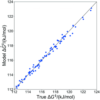Fig. 6 Parity plot showing predictions of grafting activation barriers by the kernel regression model trained on 100 grafting sites.

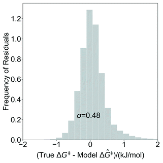
The model trained with 100 ΔG^‡ calculations was used to predict grafting barriers for all 19 368 grafting sites. After training, the only input information for each grafting site are its values of d₁, d₂, and θ. The residuals of the predictions are plotted as a distribution in Fig. 7. Nearly all residuals are within ±1 kJ mol⁻¹, and the standard deviation of the residual distribution is 0.48 kJ mol⁻¹.

Fig. 7 Distribution of residuals for a model trained on 100 grafting sites.

6.3. Identifying important local coordinates

The results in sec. 6.2. used three of five coordinates to construct the kernel regression model. Three is already a relatively compact structural parameter set, but for this model it can be reduced further. To evaluate the importance of different combinations of local coordinates, the model was retrained by systematically excluding some coordinates. Table 2 shows R² values for fits with different coordinates. Fig. 8 shows parity plots like the one in Fig. 6, but for a model based only on d₁, and for a model based on d₁ and d₂ (i.e., without θ).

Table 2 R ² values of kernel regression models with different combinations of local coordinates

Coordinates	R ^2
θ	−0.02
d 2	0.52
d 1	0.60
d 2, θ	0.52
d 1, θ	0.60
d 1, d2	0.99
d 1, d2, θ	0.99

---

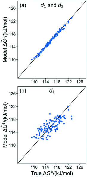Fig. 8 (a) Parity plot of the model trained with d₁ and d₂. (b) Parity plot of the model trained with d₁ only.

The model trained using d₁ and d₂ (R² = 0.99) is comparable in accuracy to the model trained using all coordinates (R² = 0.99). Clearly, d₁ and d₂ are both important for describing barriers, but θ is inconsequential as its omission does not diminish the accuracy of the kernel regression model. We can also see that the model cannot be further simplified from d₁ and d₂ dependence. The models trained on only d₁ (R² = 0.60) and d₂ (R² = 0.52) have severely diminished accuracy.

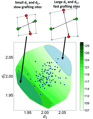
Now, using just two coordinates, we can project the grafting free energy barriers onto a 2D plot, Fig. 9. The barrier decreases monotonically with increasing d₁ or d₂. Therefore, grafting sites with large values of d₁ and d₂ react first, while grafting sites with small values of d₁ and d₂ react more slowly. We emphasize that, even with this simple model, it was not obvious a priori how structural characteristics would influence the grafting kinetics. The procedures in this paper should help to identify features of the most reactive silanol sites.

Fig. 9 Model-predicted barriers as function of d₁ and d₂. Blue dots show training set grafting sites. The figure also shows the structures of active and inactive grafting sites. Grafting sites with smaller values of d₁ and d₂ have larger barriers, while grafting sites with larger values of d₁ and d₂ have smaller barriers.

6.4. Predicting the time evolving population of grafting sites

In this section, we recompute results from section 6.1., now using the kernel regression model. We use the model based only on d₁ and d₂ and trained on just 100 randomly sampled grafting sites to predict the evolving population of unreacted silanols. The results are shown in Fig. 10a.

Fig. 10 (a) Evolving population of grafting sites predicted using a kernel regression model trained on 100 grafting sites. (b) The predicted fraction of unreacted grafting sites as a function of logarithmic time.

The training set of 100 grafting sites does not include examples of grafting sites at the extreme fast and slow grafting limits. Accordingly, the trained model does not accurately predict grafting kinetics at the extreme fast and slow limits. Fortunately, the extreme tails account for only a small portion of the total grafting sites, so important properties like the overall grafting progress are still accurately predicted by the model, Fig. 10b.

7. Conclusions

Several factors make ab initio rate calculations prohibitively difficult for single-atom catalysts grafted to amorphous supports such as silica. First, the quenched disorder of the support presents an unknown distribution of local environments. Second, grafted site abundances depend on differences in grafting kinetics at different grafting sites. Third, differences between the grafted sites can cause differences in their catalytic activity. Several investigators are working to overcome the first challenge.^71–74 This paper addresses the second challenge by combining transition state theory, kernel regression, and population balance models. A companion paper to this one addresses the third challenge.⁹³

To illustrate and test the new methodology, we introduce a simple 2D disordered lattice model of amorphous silica. The model allows us to compute the grafting rate at nearly 20 thousand grafting sites to obtain essentially exact solutions for the evolving grafting/grafted site population during grafting. Then, we trained a kernel regression model to predict grafting rates from a training set of rate calculations at just 100 grafting sites. The regression model predicted barriers with ca. ±0.5 kJ mol⁻¹ accuracy on the test set of about 20 thousand grafting sites. We also showed how the kernel regression results can identify those grafting site characteristics that most strongly influence the grafting kinetics. Finally, the trained kernel regression model was used to predict the evolving population of unreacted silanols.

In future work, we will use this framework with ab initio calculations and more realistic silica models to predict grafting rates and active site abundances during the preparation of real single-site catalysts on amorphous silica. Given a model of amorphous silica, the new algorithm should enable quantitative predictions about the grafting process and the grafted site distribution without assuming the characteristics of the most active or most abundant sites.

Conflicts of interest

There are no conflicts to declare.

Acknowledgements

We thank Bryan Goldsmith, Marco Caricato, Ward Thompson, Brian Laird and Frederick Tielens for helpful discussions. Department of Energy Basic Energy Sciences Catalysis Award DE-FG02-03ER15467 supported the kernel regression model development. National Science Foundation CBET Award 1605867 supported the population balance model. Department of Energy Computational Chemical Sciences Award DE-SC0019488 supported development of quench-disordered lattice model system. Use was made of computational facilities purchased with funds from the National Science Foundation (CNS-1725797) and administered by the Center for Scientific Computing (CSC). The CSC is supported by the California NanoSystems Institute and the Materials Research Science and Engineering Center (MRSEC; NSF DMR 1720256) at UC Santa Barbara.

References

1. K. Morokuma and D. G. Musaev, Computational Modeling for Homogeneous and Enzymatic Catalysis: A Knowledge-Base for Designing Efficient Catalysis, John Wiley & Sons, 2008.
2. T. Sperger, I. A. Sanhueza, I. Kalvet and F. Schoenebeck, Chem. Rev., 2015, 115, 9532–9586.
3. B. R. Goldsmith, T. Hwang, S. Seritan, B. Peters and S. L. Scott, J. Am. Chem. Soc., 2015, 137, 9604–9616.
4. M. Garcia-Viloca, J. Gao, M. Karplus and D. G. Truhlar, Science, 2004, 303, 186.
5. G. Voth, Computational approaches for studying enzyme mechanism, Academic Press, 2016.
6. I. Tuñón and V. Moliner, Simulating enzyme reactivity: computational methods in enzyme catalysis, Royal Society of Chemistry, 2016.
7. B. Hammer and J. K. Nørskov, in Advances in Catalysis, Academic Press, 2000, vol. 45, pp. 71–129.
8. R. B. Getman, W. F. Schneider, A. D. Smeltz, W. N. Delgass and F. H. Ribeiro, Phys. Rev. Lett., 2009, 102, 076101.
9. J. Greeley, Annu. Rev. Chem. Biomol. Eng., 2016, 7, 605–635.
10. M. Saleheen and A. Heyden, ACS Catal., 2018, 8, 2188–2194.
11. M. Salciccioli, M. Stamatakis, S. Caratzoulas and D. G. Vlachos, Chem. Eng. Sci., 2011, 66, 4319–4355.
12. S. R. Blaszkowski and R. A. van Santen, J. Phys. Chem. B, 1997, 101, 2292–2305.
13. Y.-P. Li, M. Head-Gordon and A. T. Bell, ACS Catal., 2014, 4, 1537–1545.
14. D. Newsome and M.-O. Coppens, Chem. Eng. Sci., 2015, 121, 300–312.
15. E. W. McFarland and H. Metiu, Chem. Rev., 2013, 113, 4391–4427.
16. T. Le Bahers, M. Rérat and P. Sautet, J. Phys. Chem. C, 2014, 118, 5997–6008.
17. F. Li, S. Luo, Z. Sun, X. Bao and L.-S. Fan, Energy Environ. Sci., 2011, 4, 3661–3667.
18. B. C. Knott, M. Haddad Momeni, M. F. Crowley, L. F. Mackenzie, A. W. Götz, M. Sandgren, S. G. Withers, J. Ståhlberg and G. T. Beckham, J. Am. Chem. Soc., 2014, 136, 321–329.
19. L. Masgrau and D. G. Truhlar, Acc. Chem. Res., 2015, 48, 431–438.
20. E. Brunk, J. S. Arey and U. Rothlisberger, J. Am. Chem. Soc., 2012, 134, 8608–8616.
21. B. Peters and S. L. Scott, J. Chem. Phys., 2015, 142, 104708.
22. B. R. Goldsmith, E. D. Sanderson, D. Bean and B. Peters, J. Chem. Phys., 2013, 138, 204105.
23. M. P. McDaniel, in Advances in Catalysis, ed. B. C. Gates and H. Knözinger, Academic Press, 2010, vol. 53, pp. 123–606.
24. C. Copéret, A. Comas-Vives, M. P. Conley, D. P. Estes, A. Fedorov, V. Mougel, H. Nagae, F. Núñez-Zarur and P. A. Zhizhko, Chem. Rev., 2016, 116, 323–421.
25. J. K. F. Buijink, J. J. M. van Vlaanderen, M. Crocker and F. G. M. Niele, Catal. Today, 2004, 93–95, 199–204.
26. M. F. Delley, F. Núñez-Zarur, M. P. Conley, A. Comas-Vives, G. Siddiqi, S. Norsic, V. Monteil, O. V. Safonova and C. Copéret, Proc. Natl. Acad. Sci. U. S. A., 2014, 111, 11624.
27. L. Floryan, A. P. Borosy, F. Núñez-Zarur, A. Comas-Vives and C. Copéret, J. Catal., 2017, 346, 50–56.
28. Ø. Espelid and K. J. Børve, J. Catal., 2002, 206, 331–338.
29. A. Fong, C. Vandervelden, S. L. Scott and B. Peters, ACS Catal., 2018, 8, 1728–1733.
30. A. Fong, Y. Yuan, S. L. Ivry, S. L. Scott and B. Peters, ACS Catal., 2015, 5, 3360–3374.
31. M. Gierada and J. Handzlik, J. Catal., 2018, 359, 261–271.
32. H. Guesmi and F. Tielens, J. Phys. Chem. C, 2012, 116, 994–1001.
33. C. S. Ewing, A. Bagusetty, E. G. Patriarca, D. S. Lambrecht, G. Veser and J. K. Johnson, Ind. Eng. Chem. Res., 2016, 55, 12350–12357.
34. A. M. Jystad, A. Biancardi and M. Caricato, J. Phys. Chem. C, 2017, 121, 22258–22267.
35. E. F. Vansant, P. Van Der Voort and K. C. Vrancken, Characterization and chemical modification of the silica surface, Elsevier, 1995.
36. C. J. Brinker and G. W. Scherer, Sol-gel science: the physics and chemistry of sol-gel processing, Academic press, 1990.
37. H. E. Bergna and W. O. Roberts, Colloidal silica: fundamentals and applications, CRC Press, 2005.
38. R. Brückner, J. Non-Cryst. Solids, 1970, 5, 123–175.
39. R. Brückner, J. Non-Cryst. Solids, 1971, 5, 177–216.
40. O. W. Flörke, H. A. Graetsch, F. Brunk, L. Benda, S. Paschen, H. E. Bergna, W. O. Roberts, W. A. Welsh, C. Libanati and M. Ettlinger, in Ullmann's Encyclopedia of Industrial Chemistry, John Wiley & Sons, 2000.
41. M. Atiqullah, M. N. Akhtar, A. A. Moman, A. H. Abu-Raqabah, S. J. Palackal, H. A. Al-Muallem and O. M. Hamed, Appl. Catal., A, 2007, 320, 134–143.
42. M. Oschatz, T. W. van Deelen, J. L. Weber, W. S. Lamme, G. Wang, B. Goderis, O. Verkinderen, A. I. Dugulan and K. P. de Jong, Catal. Sci. Technol., 2016, 6, 8464–8473.
43. A. Rimola, D. Costa, M. Sodupe, J.-F. Lambert and P. Ugliengo, Chem. Rev., 2013, 113, 4216–4313.
44. L. T. Zhuravlev, Colloids Surf., A, 2000, 173, 1–38.
45. S. K. Sharma, J. F. Mammone and M. F. Nicol, Nature, 1981, 292, 140–141.
46. C. J. Brinker, R. K. Brow, D. R. Tallant and R. J. Kirkpatrick, J. Non-Cryst. Solids, 1990, 120, 26–33.
47. B. Humbert, A. Burneau, J. P. Gallas and J. C. Lavalley, J. Non-Cryst. Solids, 1992, 143, 75–83.
48. J. B. Peri and A. L. Hensley, J. Phys. Chem., 1968, 72, 2926–2933.
49. Z. A. Taha, E. W. Deguns, S. Chattopadhyay and S. L. Scott, Organometallics, 2006, 25, 1891–1899.
50. S. D. Fleischman and S. L. Scott, J. Am. Chem. Soc., 2011, 133, 4847–4855.
51. A. O. Bouh, G. L. Rice and S. L. Scott, J. Am. Chem. Soc., 1999, 121, 7201–7210.
52. X. Gao, S. R. Bare, J. L. G. Fierro, M. A. Banares and I. E. Wachs, J. Phys. Chem. B, 1998, 102, 5653–5666.
53. A. Kytökivi and S. Haukka, J. Phys. Chem. B, 1997, 101, 10365–10372.
54. E. W. Deguns, Z. Taha, G. D. Meitzner and S. L. Scott, J. Phys. Chem. B, 2005, 109, 5005–5011.
55. H. Zhu, S. Ould-Chikh, H. Dong, I. Llorens, Y. Saih, D. H. Anjum, J.-L. Hazemann and J.-M. Basset, ChemCatChem, 2015, 7, 3332–3339.
56. J. Jarupatrakorn and T. D. Tilley, J. Am. Chem. Soc., 2002, 124, 8380–8388.
57. J. M. Fraile, J. I. García, J. A. Mayoral and E. Vispe, J. Catal., 2005, 233, 90–99.
58. L. Zhong, M.-Y. Lee, Z. Liu, Y.-J. Wanglee, B. Liu and S. L. Scott, J. Catal., 2012, 293, 1–12.
59. K. Fukudome, N.-o. Ikenaga, T. Miyake and T. Suzuki, Catal. Sci. Technol., 2011, 1, 987–998.
60. M. K. Samantaray, E. Pump, A. Bendjeriou-Sedjerari, V. D'Elia, J. D. A. Pelletier, M. Guidotti, R. Psaro and J.-M. Basset, Chem. Soc. Rev., 2018, 47, 8403–8437.
61. J. Handzlik, R. Grybos and F. Tielens, J. Phys. Chem. C, 2013, 117, 8138–8149.
62. M. Cavalleri, K. Hermann, A. Knop-Gericke, M. Hävecker, R. Herbert, C. Hess, A. Oestereich, J. Döbler and R. Schlögl, J. Catal., 2009, 262, 215–223.
63. R. Z. Khaliullin and A. T. Bell, J. Phys. Chem. B, 2002, 106, 7832–7838.
64. T.-H. Wang, J. L. Gole, M. G. White, C. Watkins, S. C. Street, Z. Fang and D. A. Dixon, Chem. Phys. Lett., 2011, 501, 159–165.
65. N. R. Jaegers, C. Wan, M. Y. Hu, M. Vasiliu, D. A. Dixon, E. Walter, I. E. Wachs, Y. Wang and J. Z. Hu, J. Phys. Chem. C, 2017, 121, 6246–6254.
66. J. Handzlik, Int. J. Quantum Chem., 2007, 107, 2111–2119.
67. L. W. Chung, W. M. C. Sameera, R. Ramozzi, A. J. Page, M. Hatanaka, G. P. Petrova, T. V. Harris, X. Li, Z. Ke, F. Liu, H.-B. Li, L. Ding and K. Morokuma, Chem. Rev., 2015, 115, 5678–5796.
68. T. P. M. Goumans, C. R. A. Catlow and W. A. Brown, J. Chem. Phys., 2008, 128, 134709.
69. J. Handzlik and J. Ogonowski, J. Phys. Chem. C, 2012, 116, 5571–5584.
70. J. Gomes, P. M. Zimmerman, M. Head-Gordon and A. T. Bell, J. Phys. Chem. C, 2012, 116, 15406–15414.
71. C. S. Ewing, S. Bhavsar, G. Veser, J. J. McCarthy and J. K. Johnson, Langmuir, 2014, 30, 5133–5141.
72. P. Ugliengo, M. Sodupe, F. Musso, I. J. Bush, R. Orlando and R. Dovesi, Adv. Mater., 2008, 20, 4579–4583.
73. A. Comas-Vives, Phys. Chem. Chem. Phys., 2016, 18, 7475–7482.
74. F. Tielens, C. Gervais, J. F. Lambert, F. Mauri and D. Costa, Chem. Mater., 2008, 20, 3336–3344.
75. B. Peters, S. L. Scott, A. Fong, Y. Wang and A. E. Stiegman, Proc. Natl. Acad. Sci. U. S. A., 2015, 112, E4160.
76. N. M. Peek, D. B. Jeffcoat, C. Moisii, L. van de Burgt, S. Profeta, S. L. Scott and A. E. Stiegman, J. Phys. Chem. C, 2018, 122, 4349–4358.
77. S. Lwin, Y. Li, A. I. Frenkel and I. E. Wachs, ACS Catal., 2016, 6, 3061–3071.
78. B. Peters, Reaction rate theory and rare events, Elsevier, 2017.
79. J. K. Nørskov, F. Studt, F. Abild-Pedersen and T. Bligaard, Fundamental Concepts in Heterogeneous Catalysis, Wiley, 2014.
80. B. Peters, J. Phys. Chem. B, 2015, 119, 6349–6356.
81. I. Chorkendorff and J. W. Niemantsverdriet, Concepts of modern catalysis and kinetics, John Wiley & Sons, 2017.
82. M. Boudart and G. Djéga-Mariadassou, Kinetics of heterogeneous catalytic reactions, Princeton University Press, 2014.
83. R. A. Van Santen and M. Neurock, Molecular heterogeneous catalysis: a conceptual and computational approach, John Wiley & Sons, 2009.
84. F. Jensen, Introduction to computational chemistry, John wiley & sons, 2017.
85. J. E. Leffler, Science, 1953, 117, 340–341.
86. P. C. Mahalanobis, Proc. Natl. Inst. Sci. India, 1936, 2, 49–55.
87. T. Hofmann, B. Schölkopf and A. J. Smola, Ann. Stat., 2008, 36, 1171–1220.
88. M. Mohri, A. Rostamizadeh and A. Talwalkar, Foundations of machine learning, MIT press, 2018.
89. K. Q. Weinberger and G. Tesauro, Metric learning for kernel regression, International Conference on Artificial Intelligence and Statistics, 2007.
90. G. Strang and S. Strang, Linear Algebra and Its Applications, Thomson, Brooks/Cole, 2006.
91. J. Nocedal and S. Wright, Numerical optimization, Springer Science & Business Media, 2006.
92. C. J. Carey and Y. Tang, metric-learn, 2015.
93. C. Vandervelden, S. A. Khan, S. L. Scott and B. Peters, React. Chem. Eng., 2019 10.1039/C9RE00356H.

---

Footnotes

† Electronic supplementary information (ESI) available: Setting parameters in model chemistry and testing set error for the kernel regression model. See DOI: 10.1039/c9re00357f

‡ Authors with equal contribution.

---