Site-averaged kinetics for catalysts on amorphous supports: an importance learning algorithm†
Craig A.
Vandervelden‡
 a,
Salman A.
Khan‡
 a,
Susannah L.
Scott
 ab and
Baron
Peters
 *cd
*cd
aDepartment of Chemical Engineering, University of California, Santa Barbara, California 93106-5080, USA
bDepartment of Chemistry, University of California, Santa Barbara, California 93106-5080, USA
cDepartment of Chemical and Biomolecular Engineering, University of Illinois at Urbana-Champaign, Urbana, Illinois 61801, USA. E-mail: baronp@illinois.edu
dDepartment of Chemistry, University of Illinois at Urbana-Champaign, Urbana, Illinois 61801, USA
First published on 31st October 2019
Abstract
Ab initio calculations have greatly advanced our understanding of homogeneous catalysts and crystalline heterogeneous catalysts. In contrast, amorphous heterogeneous catalysts remain poorly understood. The principal difficulties include (i) the nature of the disorder is quenched and unknown; (ii) each active site has a different local environment and activity; (iii) active sites are rare, often less than ∼20% of potential sites, depending on the catalyst and its preparation method. Few (if any) studies of amorphous heterogeneous catalysts have ever attempted to compute site-averaged kinetics, because the exponential dependence on variable activation energy requires an intractable number of ab initio calculations to converge. We present a new algorithm using machine learning techniques (metric learning kernel regression) and importance sampling to efficiently learn the distribution of activation energies. We demonstrate the algorithm by computing the site-averaged activity for a model amorphous catalyst with quenched disorder.
Introduction
A recent surge of interest in atomically-dispersed “single atom” catalysts is driven by their unique and potentially selective reactivity,1–3 and by sustainability efforts that seek to minimize use of scarce elements and maximize atom economy.4–6 Among single atom catalysts, those which are chemically bonded to a thermally robust oxide support like silica are especially resistant to deactivation by sintering.7,8 Moreover, grafting strategies that promote selective reaction of the catalyst precursor at specific surface sites may help to minimize differences between grafted metal sites. Well-studied catalysts that are comprised of single metal atoms grafted onto amorphous silica include chromocenes or chromates for olefin polymerization,9–11 titanium and tantalum complexes for olefin epoxidation,12 molybdates for methanol dehydration,13 and vanadates for partial oxidation of methanol.14Investigators have occasionally drawn comparisons between the metal atoms present in the active sites in enzymes, and metal atoms grafted onto silica surfaces.12 There are similarities, but there are also important differences. Each enzyme molecule of a given type is the same, while each metal atom on amorphous silica resides in a unique ligand environment. These non-uniform environments can result in metal atoms with non-uniform catalytic properties, including a range of activities, selectivities, adsorption constants, and even different spectroscopic features. When the sites have variable activities, a minority of the sites may contribute most of the overall catalyst activity. Indeed, active site counting experiments confirm that only a small fraction of sites in a heterogeneous catalyst is typically active.15–18 This poses an extraordinary difficulty in experimental as well as theoretical studies of these catalysts. Powerful characterization tools (NMR, EXAFS, IR, Raman, etc.) generally provide the strongest signals for the most common sites, and these are likely inactive.11
If we could understand the mechanisms of these catalysts, we might systematically work to improve them.19 In some applications like olefin polymerization, where the catalysts are not recovered from the polymer product, one might even use mechanistic understanding to design catalysts with a desired activity distribution capable of generating polymer with a desired molecular weight distribution.
Our first paper introduced a method to predict the distribution of sites that emerges from grafting a precursor onto an amorphous support.20 The simple model system consisted of a quenched-disordered lattice (to represent the amorphous silica support), surface functional groups (representing pairs or nests of hydroxyl groups) to which a metal complex can be grafted, and a microkinetic model for each grafted site with rate parameters that depend on the site characteristics. Much like in an ab initio study, computing activation barriers for the model system requires geometry optimizations of intermediates. Our realistic but simple model allowed us to focus on developing the importance sampling and machine learning tools, without being distracted by controversies about the mechanisms of these catalysts.
Starting from the simple model and the grafted site population described in our first paper,20 this second paper aims to compute an average over sites to predict the overall kinetics. Since the turnover frequencies at individual sites vary exponentially with the activation energy, even a small variance in the activation energy leads to an enormous variance in site-specific activities. Such exponential averages are notoriously difficult to converge with standard sampling tools,21–23 but importance sampling methods can dramatically accelerate convergence. The ideal importance sampling algorithm24 requires activation energies for each site, but these activation energies are not known a priori. Each activation energy must be obtained through costly ab initio calculations. Because of this limitation, typical approaches calculate just one25,26 or a small handful of sites27–34 – far too few to converge site-averaged predictions of kinetic properties.35 Kernel regression tools can use a modest set of ab initio calculations to predict activation energies that have not actually been computed. This paper shows how importance sampling and machine learning can be combined to generate site-averaged predictions efficiently.
In the remainder of this paper, we discuss model elementary steps and a rate law for a catalytic reaction with our simple model system. We briefly review the kernel regression tools (from our first paper) that predict activation energies. We combine the importance sampling and kernel regression tools into an “importance learning algorithm”. We then use the new algorithm to identify characteristics of highly active sites and to estimate site-averaged activation energies. Finally, we compare the efficiency of importance sampling estimates to straightforward sampling.
Model for amorphous support and grafted sites
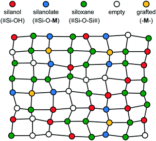
Our previous paper described the creation of a disordered, functionalized lattice model to approximate the non-uniform silanol sites and siloxane environments on the surface of amorphous SiO2. That paper also considered a kinetic model for grafting of metal atoms onto the silanol sites. All sites with two silanol neighbors and two siloxane neighbors on opposite sides were eligible grafting sites in the model. A schematic of the simple model is shown in Fig. 1.This paper uses the distribution of non-uniform grafted sites, like those shown in Fig. 1, as its starting point. We assume that grafting has occurred at all eligible sites, but one could modify the starting distribution (using methods in the previous paper20) to investigate lower catalyst loadings.
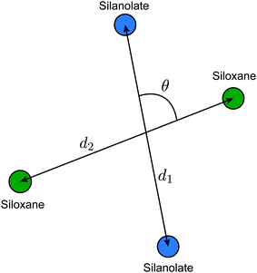
The discussion below invokes bonds between metal atoms and adsorbates, as well as the oxygen atoms of the silanol and siloxane sites. However, the local environment of each site (before grafting and during catalysis) is described entirely by the positions of atoms in the silica support surrounding the metal center. The coordinates used to describe the local environment are shown in Fig. 2. They are: (i) the distance between siloxane groups, d1, (ii) the distance between silanolate groups, d2, and (iii) the angle between the silanolate and siloxane groups, θ.
The selected coordinates are nearly orthogonal in the sense that their gradients have little or no overlap. Note, however, that the coordinates are incomplete. For a grafting site on our two dimensional surface model, the four nearest neighbors are fully described by five internal coordinates (8–2×(center of mass)–1×(rotation)). We use only three coordinates in the kernel regression model, and the results below will show that just two of these coordinates are sufficient to predict site-averaged kinetics. We also emphasize that some calculations below involve other coordinates at intermediate stages, but that the overall kinetics and the kinetics of individual sites ultimately depend only on the coordinates in Fig. 2.
Model for catalysis at grafted sites
We consider a simple model of a catalyst site, M*, comprised of a metal center M and its surrounding support environment, *. We will consider the case in which the catalytic reaction at each site has the same rate-limiting step and the same most abundant surface intermediate (MASI). We further assume that the site does not deactivate. The model reaction has a simple Langmuir–Hinshelwood mechanism:We further assume that
(i) the equilibrium constant K for adsorption of reactant A depends on the local environment of site i, xi,
(ii) the adsorbed molecule A (AM*) is irreversibly converted into the gas phase product B and a bare site M*,
(iii) K(x)cA ≪ 1 for all sites, so that the bare site M* is the MASI.
The bond strengths chosen in this work, described below, ensure that these three assumptions are true for all sites. Fig. 3 depicts the Langmuir–Hinshelwood mechanism and the three simplifying assumptions for the simple model system in this work.
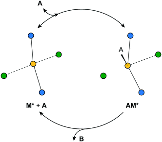 | ||
| Fig. 3 The equilibrated adsorption step and irreversible chemical reaction steps for the model reaction A → B, and the M* sites described in this work. | ||
The Langmuir–Hinshelwood mechanism leads to a rate law of form
 | (1) |
 | (2) |
| k(x) = k2K(x). | (3) |
The apparent rate constant k(x) depends on the local site geometry through K(x). The adsorption constant is
 | (4) |
 | (5) |
The site-dependent enthalpy of adsorption, ΔH(x), is modeled by
| ΔH(x) = VAM*(x) − (VM*(x) + εA + kBT) | (6) |
![[triple bond, length as m-dash]](https://www.rsc.org/images/entities/char_e002.gif) bond energies and M⋯(OSi
bond energies and M⋯(OSi![[triple bond, length as m-dash]](https://www.rsc.org/images/entities/char_e002.gif) )2 bond energies. Specifically, the individual interaction energies are
)2 bond energies. Specifically, the individual interaction energies are| εi(r) = Di(1 − exp[−ai(r − ri,eq)2])− Di | (7) |
 | (8) |
![[triple bond, length as m-dash]](https://www.rsc.org/images/entities/char_e002.gif) bonds, ri is the metal–oxygen bond distance,
bonds, ri is the metal–oxygen bond distance,  is the energy of the M⋯(OSi
![[triple bond, length as m-dash]](https://www.rsc.org/images/entities/char_e002.gif) )2 metal–siloxane bond, and
)2 metal–siloxane bond, and  is the metal–siloxane bond distance.
We model adsorption of A onto the grafted metal center as an M–A bond with energy εM–A. The length of the M–A bond is not explicitly optimized. Instead, we assume that the M–A bond displaces the longest and most weakly-coordinated siloxane (M⋯(OSi![[triple bond, length as m-dash]](https://www.rsc.org/images/entities/char_e002.gif) )2) from M. The displaced siloxane can still exert a repulsive interaction on M. We model the close-range repulsion with a Weeks–Chandler–Andersen potential:36
)2) from M. The displaced siloxane can still exert a repulsive interaction on M. We model the close-range repulsion with a Weeks–Chandler–Andersen potential:36
| εWCAAM⋯O(r) = DAM⋯O(1 − exp [−aAM⋯O(r − rAM⋯O,eq)2]) | (9) |
 | (10) |
With these definitions, eqn (6) presents a geometry optimization problem much like that encountered in ab initio calculations. The interior atoms must be optimized subject to constraints on peripheral atoms around the metal center. The equilibrium configurations of M* and AM* are found by changing the M atom position with fixed silanolate and siloxane group positions to minimize (8) and (10), respectively. This procedure creates a collection of model sites with quenched disorder and limited local flexibility, somewhat like a real amorphous catalyst.
Parameter selection
The quenched disordered lattice was created by starting with a square lattice with spacing 1. Random displacements of the lattice sites were drawn from an isotropic 2D Gaussian distribution with σ2lattice = 0.00022 in the x and y directions. We used the same fractions of silanol, siloxane, and empty sites (fsilanol= 0.3, fsiloxane = 0.3, and fempty = 0.4) as our previous paper.20 All rate calculations in this work were performed for a temperature of 300 K and a reactant pressure of 1 atm. The metal-adsorbate bond dissociation energy was modeled as the Cr–C bond dissociation energy for a (![[triple bond, length as m-dash]](https://www.rsc.org/images/entities/char_e002.gif) SiO)2CrIII alkyl site – the widely accepted active site for Cr/SiO2 olefin polymerization catalysts.11,37 Based on DFT calculations (section S1†) and reported values for the Cr–C bond,38 we set εM–A = 160 kJ mol−1. A list of the parameters and their values are summarized in Table 1.
SiO)2CrIII alkyl site – the widely accepted active site for Cr/SiO2 olefin polymerization catalysts.11,37 Based on DFT calculations (section S1†) and reported values for the Cr–C bond,38 we set εM–A = 160 kJ mol−1. A list of the parameters and their values are summarized in Table 1.
| Parameter | Value |
|---|---|
| T | 300 K |
| P A | 1 atm |
| ΔH‡ | 65 kJ mol−1 |
| σ 2 lattice | 0.00022 |
| f silanol | 0.3 |
| f siloxane | 0.3 |
| f empty | 0.4 |
| D M⋯O | 120 kJ mol−1 |
| a M⋯O | 1.3 |
![[r with combining circumflex]](https://www.rsc.org/images/entities/i_char_0072_0302.gif) M⋯O,eq
M⋯O,eq
|
1.16 |
| D M–O | 500 kJ mol−1 |
| a M–O | 1.7 |
![[r with combining circumflex]](https://www.rsc.org/images/entities/i_char_0072_0302.gif) M–O,eq
M–O,eq
|
1.0 |
| ε A | 0 |
| ε M–A | 160 kJ mol−1 |
Site-averaged kinetics
Each metal site has a unique environment, and the different environments lead to a distribution of kinetic properties. For example, the sites will exhibit a distribution of turnover frequencies and activation energies. In contrast, a conventional experiment measures just one site-averaged value for each kinetic property. In this paper, we focus on the site-averaged activation energy. From eqn (2)–(5), the activation energy for site i is | (11) |
Naively, one might estimate Ea(x) for a large sample of sites and then average them to obtain the site-averaged activation energy. This straightforward average does not give the correct value, even in the limit of large sample sizes. The correct site-averaged activation energy,40 〈Ea〉k is obtained from a derivative of the site-averaged rate:
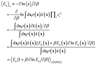 | (12) |
In this work, we ignore the temperature dependence of Ea. In practice, the rates at individual sites cannot be probed, nor are the temperature intervals in which the rates are measured wide enough to see definitive curvature in the Arrhenius plot. We also expect the correction to be small. Using Ea from eqn (11), β![[thin space (1/6-em)]](https://www.rsc.org/images/entities/char_2009.gif) ∂ln
∂ln![[thin space (1/6-em)]](https://www.rsc.org/images/entities/char_2009.gif) Ea/∂β = 2β−1, which will be relatively small compared to a typical Ea(x). Moreover, we anticipate that β
Ea/∂β = 2β−1, which will be relatively small compared to a typical Ea(x). Moreover, we anticipate that β![[thin space (1/6-em)]](https://www.rsc.org/images/entities/char_2009.gif) ∂ln
∂ln![[thin space (1/6-em)]](https://www.rsc.org/images/entities/char_2009.gif) Ea/∂β term will be similar across different sites, so that conclusions about characteristics of highly active and abundant sites will be unaffected. Using eqn (2)–(5), the derivatives and integrations yield:
Ea/∂β term will be similar across different sites, so that conclusions about characteristics of highly active and abundant sites will be unaffected. Using eqn (2)–(5), the derivatives and integrations yield:
| 〈Ea〉k = 〈ΔH(x) + ΔH‡ + 2kBT〉k. | (13) |
The first strategy is to randomly choose sites from ρ(x) and reweight each of them by k(x) when computing the average:
 | (14) |
The second strategy is to directly sample sites according to probability weight ρ(x)k(x). This is difficult, because we do not know k(x) precisely prior to performing ab initio calculations at x. However, if such a sampling algorithm could be devised (see below), the site-averaged activation energy would become a simple arithmetic average:
 | (15) |
 | (16) |
 | (17) |
Kernel regression
To sample the distribution ρ(x)k(x) starting from a large collection of sites, i.e., from ρ(x), we require preliminary estimates for k(x) at each site. Given accurate calculations as training data at a modest collection of sites, kernel regression can estimate Ea(x) at all the remaining sites.41,42 The estimated activation energy at site with environment xi is a weighted average of the training data, eqn (18): | (18) |
| wij = exp[−d2(xi, xj)] | (19) |
| d2(xi, xj) = (xi − xj)TS(xi − xj). | (20) |
Importance learning algorithm
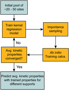
The sections above described rate calculations at individual sites, an importance sampling procedure, and a kernel regression (machine learning) procedure. This section integrates all of these components into one “importance learning” algorithm. Importance learning simultaneously accumulates training data, builds the kernel regression model, and focuses computational effort on kinetically important sites with low activation barriers. The algorithm is shown in Fig. 4.Note that the importance sampling and kernel regression procedures mutually depend on each other. The kernel regression model guides the importance sampling to kinetically important sites. Meanwhile, the accumulated sample of sites and rate calculations teach kernel regression to make accurate preliminary rate predictions.
To compute kinetic properties, precise rate calculations for less active sites are not important, but we need their populations to predict kinetic properties like the overall rate and the fraction of active sites. Therefore, the kernel regression model should also learn to make approximate predictions for inactive sites. For this reason, the importance learning algorithm begins with rate calculations at a collection of randomly sampled sites. We verified that an initial training set of 20–50 randomly chosen sites is adequate (section S4 in the ESI†).
Results
Because the model system is extremely simple, an accurate site-averaged activation energy can be directly calculated without importance learning. Using results for ∼20![[thin space (1/6-em)]](https://www.rsc.org/images/entities/char_2009.gif) 000 sites, we computed the activation energy distribution:
000 sites, we computed the activation energy distribution: | (21) |
 | (22) |
Fig. 5 shows the essentially exact distributions ![[small rho, Greek, tilde]](https://www.rsc.org/images/entities/i_char_e0e4.gif) (Ea) and
(Ea) and ![[small rho, Greek, tilde]](https://www.rsc.org/images/entities/i_char_e0e4.gif) k(Ea). The activation energy distribution has support45 over a range of about 40 kJ mol−1. The site-averaged activation energy is 40.4 kJ mol−1, about 13 kJ mol−1 below the (incorrect) average without k-weighting. These results serve as benchmarks for testing the importance learning algorithm.
k(Ea). The activation energy distribution has support45 over a range of about 40 kJ mol−1. The site-averaged activation energy is 40.4 kJ mol−1, about 13 kJ mol−1 below the (incorrect) average without k-weighting. These results serve as benchmarks for testing the importance learning algorithm.
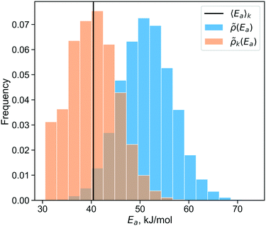 | ||
| Fig. 5 Distribution of activation energies (blue) and the rate-weighted activation energy distribution (orange). The solid line shows the site-averaged activation energy. | ||
To start the importance learning algorithm, we began with an initial training set of fifty randomly chosen sites. The initial kernel regression model was optimized to minimize the leave-one-out errors. Within this initial training set, the kernel regression model predicts activation energies with a standard error σ ≈ 0.8 kJ mol−1. Fig. 6 shows how the predicted activation energies compare to the true (precisely computed viaeqn (11)) activation energies for individual sites.
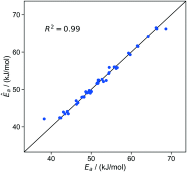 | ||
Fig. 6 Parity plot of predicted activation barriers vs. true activation barriers at individual sites. Predictions are from leave-one-out optimization of kernel regression models based on the initial training set of 50 sites. The residuals for all ∼20![[thin space (1/6-em)]](https://www.rsc.org/images/entities/char_2009.gif) 000 sites are approximately Gaussian distributed, with a standard deviation of approximately 0.7 kJ mol−1 (Fig S3†). 000 sites are approximately Gaussian distributed, with a standard deviation of approximately 0.7 kJ mol−1 (Fig S3†). | ||
At each iteration of the importance learning algorithm, the activation energy distributions ![[small rho, Greek, tilde]](https://www.rsc.org/images/entities/i_char_e0e4.gif) (Ea) and
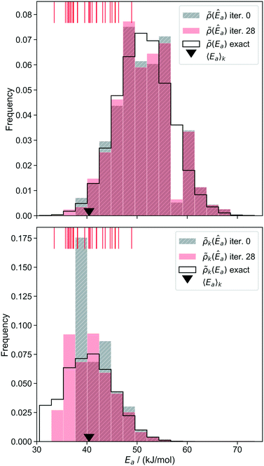
(Ea) and ![[small rho, Greek, tilde]](https://www.rsc.org/images/entities/i_char_e0e4.gif) k(Ea) can be predicted using the kernel regression model. After each iteration, the new calculations are appended to the training set. As more training data is accumulated (primarily at low activation energies), the estimated Ea distributions should become more like the true distribution in the kinetically important range of activation energies. As a corollary, the site-averaged activation energy should also converge to the correct value. Fig. 7 shows the predicted distributions at the 0th and 28th iterations of importance learning (the latter being the iteration at which the standard error decreases below 0.75 kJ mol−1). A rug shows that the activation energies of the importance sampled sites are indeed centered over the main support of
k(Ea) can be predicted using the kernel regression model. After each iteration, the new calculations are appended to the training set. As more training data is accumulated (primarily at low activation energies), the estimated Ea distributions should become more like the true distribution in the kinetically important range of activation energies. As a corollary, the site-averaged activation energy should also converge to the correct value. Fig. 7 shows the predicted distributions at the 0th and 28th iterations of importance learning (the latter being the iteration at which the standard error decreases below 0.75 kJ mol−1). A rug shows that the activation energies of the importance sampled sites are indeed centered over the main support of ![[small rho, Greek, tilde]](https://www.rsc.org/images/entities/i_char_e0e4.gif) k(Êa).
k(Êa).
Prior to importance learning, the initial training set contained only one site with an activation energy under 40 kJ mol−1. Importance learning discovers sites with activation energies below 40 kJ mol−1, which dominate the overall kinetics. After 28 iterations of importance learning, the low activation energy tail of the predicted ![[small rho, Greek, tilde]](https://www.rsc.org/images/entities/i_char_e0e4.gif) (Êa) closely resembles that of the exact
(Êa) closely resembles that of the exact ![[small rho, Greek, tilde]](https://www.rsc.org/images/entities/i_char_e0e4.gif) (Ea). More importantly, the main support of the predicted
(Ea). More importantly, the main support of the predicted ![[small rho, Greek, tilde]](https://www.rsc.org/images/entities/i_char_e0e4.gif) k(Êa) closely resembles that of the exact
k(Êa) closely resembles that of the exact ![[small rho, Greek, tilde]](https://www.rsc.org/images/entities/i_char_e0e4.gif) k(Ea). Both distributions are inaccurately predicted at high activation energies, but these sites make vanishingly small contributions to the observed kinetics. They only need to be counted in the normalization of
k(Ea). Both distributions are inaccurately predicted at high activation energies, but these sites make vanishingly small contributions to the observed kinetics. They only need to be counted in the normalization of ![[small rho, Greek, tilde]](https://www.rsc.org/images/entities/i_char_e0e4.gif) (Ea) to predict the kinetic properties.
(Ea) to predict the kinetic properties.
Fig. 8 shows the convergence of 〈Ea〉k estimates from importance sampling using standard errors. A higher degree of confidence could also be computed using eqn (16).
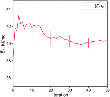 | ||
Fig. 8 The importance learning algorithm converges to within 0.75 kJ mol−1 of the correct site-averaged Ēa in 28 iterations. By comparison, a reweighted random sample requires about 200![[thin space (1/6-em)]](https://www.rsc.org/images/entities/char_2009.gif) 000 samples to compute Ẽa with the same level of confidence (section S5†). 000 samples to compute Ẽa with the same level of confidence (section S5†). | ||
Identifying characteristics of active sites
In real applications, optimizing the Mahalonobis matrix is inexpensive compared to generating training data from ab initio calculations. Therefore, an importance learning calculation can include all potentially important coordinates. However, a central goal of these calculations is to discover those few key characteristics that distinguish active from inactive sites. Intuition would suggest that the most important coordinates can be identified from the largest diagonal elements in the Mahalonobis matrix. The optimized matrix obtained in this work, using d1, d2, and θ, is: | (23) |
In general, the diagonal matrix elements are not reliable indicators of the most important structural characteristics. For example, the diagonal matrix elements change magnitude depending on the units used to represent the coordinates. In addition, diagonal matrix elements indicate sensitivity to local structural changes. They do not account for differences in the extent to which sites vary along different structural coordinates within the global ensemble of sites. Off-diagonal matrix elements may also be important. Large off-diagonal matrix elements may indicate that special combinations of the coordinates are important. Alternatively, off-diagonal elements may compensate for non-orthogonality or redundancy in the set of trial coordinates. The latter complications can be avoided by choosing coordinates that are orthogonal, in the sense:
 | (24) |
More general guidelines are that
(i) Good coordinates should suffice to predict differences in activity over the region with support in distribution ρ(x)k(x).
(ii) The kernel regression model should predict activation energies with errors that are much smaller than the range of activation energies in ![[small rho, Greek, tilde]](https://www.rsc.org/images/entities/i_char_e0e4.gif) k(Ea).
k(Ea).
These two guidelines suggest ranking models according to the fraction of the actual Ea variance that is explained by the model. In linear regression, this is the familiar R2 statistic. Models that include more input coordinates will generally give larger R2 values, but small models are preferred, as long as they give accurate site-averaged rate predictions. The fit quality of the kernel regression models trained on different sets of coordinates are shown in Fig. 9.
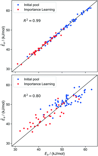 | ||
| Fig. 9 Parity plot of model trained with d1, d2 (top) and d1, θ (bottom) at iteration 30 of the importance learning algorithm. As shown in Table 2, d1 and d2 are sufficient (without the extra variable θ) to allow kernel regression to predict activation energies across the range of values. | ||
| Coordinates | R 2 |
|---|---|
| d 1 | 0.80 |
| d 2 | 0.16 |
| θ | −0.03 |
| d 1, d2 | 0.99 |
| d 1, θ | 0.82 |
| d 2, θ | 0.34 |
| d 1, d2, θ | 0.99 |
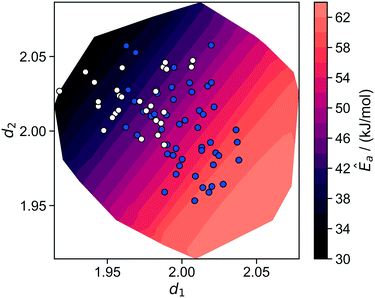
The R2 values identify θ as a kinetically unimportant structural characteristic. The kernel regression model trained only on θ completely fails to make predictions based on the local environment. Models based only on d1 or d2 begin to predict coarse trends in the activation energies. The model trained using d1 and d2 together makes extremely accurate predictions across the whole range of activation energies. Note that d1 and d2 are just two of the five total coordinates that define the local site environment. The model-predicted Ea is plotted as a function of d1 and d2 in Fig. 10. This plot reveals that d1 and d2 compensate for each other in active sites. Among sites with the same activation energy, one length increases while the other decreases. Fig. 10 also illustrates that the most active sites have shorter d1 (silanolate–silanolate) distances and longer d2 (O–O distance of the siloxane ligands) distances relative to the unperturbed distance of 2.00.
Conclusions
Several industrially important or promising catalysts are single metal atoms grafted onto an amorphous support such as silica. These catalysts tend to be poorly understood because the amorphous support gives each site a unique local environment. Moreover, the distribution of disordered environments around each site is quenched, history dependent, and thus largely unpredictable. Each site has a different activation energy, and the variance in activation energies is exponentially magnified in the distribution of activities. Accordingly, active sites tend to be rare, with a small minority of sites accounting for most of the catalytic activity. The small fraction of active sites hampers both experimental characterization and theoretical modeling efforts.This paper presented an importance learning algorithm to overcome the theoretical challenges of modeling the activity of such catalysts. It combines machine learning techniques (kernel regression) and importance sampling techniques (to focus effort on the most active and abundant sites). To illustrate the algorithm, we developed a simple model of a Langmuir–Hinshelwood reaction at sites on a quenched and disordered support. We used the algorithm to compute the site-averaged activation energy.
The algorithm rapidly converged estimates of the site-averaged Ea with uncertainties less than 0.75 kJ mol−1, even though the individual sites in the model have activation energies that span a range of nearly 40 kJ mol−1. Estimating the site-averaged Ea with the same level of confidence as importance learning requires through standard sampling methods requires 200![[thin space (1/6-em)]](https://www.rsc.org/images/entities/char_2009.gif) 000 samples (compared to ∼75 samples in the importance learning algorithm) for this system. Furthermore, the kernel regression model generated by the algorithm can accurately predict the activation energies using just two structural characteristics of the local environment. The new importance learning algorithm, if combined with ab initio calculations and realistic models of amorphous silica, should enable the first rigorous site-averaged computational studies and quantitative predictions for this important family of catalysts.
000 samples (compared to ∼75 samples in the importance learning algorithm) for this system. Furthermore, the kernel regression model generated by the algorithm can accurately predict the activation energies using just two structural characteristics of the local environment. The new importance learning algorithm, if combined with ab initio calculations and realistic models of amorphous silica, should enable the first rigorous site-averaged computational studies and quantitative predictions for this important family of catalysts.
Conflicts of interest
There are no conflicts to declare.Acknowledgements
We thank Bryan Goldsmith, Marco Caricato, Ward Thompson, Brian Laird and Frederick Tielens for helpful discussions. Department of Energy Basic Energy Sciences Catalysis Award DE-FG02-03ER15467 supported the kernel regression model development. National Science Foundation CBET Award 1605867 supported the importance learning algorithm development. Department of Energy Computational Chemical Sciences Award DE-SC0019488 supported development of quench-disordered lattice model system. Use was made of computational facilities purchased with funds from the National Science Foundation (CNS-1725797) and administered by the Center for Scientific Computing (CSC). The CSC is supported by the California NanoSystems Institute and the Materials Research Science and Engineering Center (MRSEC; NSF DMR 1720256) at UC Santa Barbara.Notes and references
- X. Zhang, H. Shi and B. Q. Xu, Angew. Chem., Int. Ed., 2005, 44, 7132–7135 CrossRef CAS PubMed.
- S. F. J. Hackett, R. M. Brydson, M. H. Gass, I. Harvey, A. D. Newman, K. Wilson and A. F. Lee, Angew. Chem., Int. Ed., 2007, 46, 8593–8596 CrossRef CAS PubMed.
- H. Wei, X. Liu, A. Wang, L. Zhang, B. Qiao, X. Yang, Y. Huang, S. Miao, J. Liu and T. Zhang, Nat. Commun., 2014, 5634 CAS.
- J. M. Thomas, R. Raja and D. W. Lewis, Angew. Chem., Int. Ed., 2005, 44, 6456–6482 CrossRef CAS PubMed.
- A. Wang, J. Li and T. Zhang, Nat. Rev. Chem., 2018, 2, 65–81 CrossRef CAS.
- M. Flytzani-Stephanopoulos and B. C. Gates, Annu. Rev. Chem. Biomol. Eng., 2012, 545–574 CrossRef CAS PubMed.
- M. P. McDaniel and M. B. Welch, J. Catal., 1983, 82, 98–109 CrossRef CAS.
- S. Maksasithorn, P. Praserthdam, K. Suriye and D. P. Debecker, Microporous Mesoporous Mater., 2015, 213, 125–133 CrossRef CAS.
- L. Carrick Wayne, J. Turbett Robert, J. Karol Frederick, L. Karapinka George, S. Fox Adrian and N. Johnson Robert, J. Polym. Sci., Part A-1: Polym. Chem., 1972, 10, 2609–2620 CrossRef.
- K. H. Theopold, Acc. Chem. Res., 1990, 23, 263–270 CrossRef CAS.
- M. P. McDaniel, Adv. Catal., 2010, 53, 123–606 CAS.
- D. A. Ruddy and T. D. Tilley, J. Am. Chem. Soc., 2008, 130, 11088–11096 CrossRef CAS PubMed.
- I. J. Shannon, T. Maschmeyer, R. D. Oldroyd, G. Sankar, J. M. Thomas, H. Pernot, J. P. Balikdjian and M. Che, J. Chem. Soc., Faraday Trans., 1998, 94, 1495–1499 RSC.
- W. C. Vining, J. Strunk and A. T. Bell, J. Catal., 2012, 281, 222–230 CrossRef.
- K. Amakawa, S. Wrabetz, J. Kröhnert, G. Tzolova-Müller, R. Schlögl and A. Trunschke, J. Am. Chem. Soc., 2012, 134, 11473 CrossRef PubMed.
- M. P. McDaniel and S. J. Martin, J. Phys. Chem., 1991, 95, 3289–3293 CrossRef CAS.
- Y. Chauvin and D. Commereuc, J. Chem. Soc., Chem. Commun., 1992, 462–464 RSC.
- J. G. Howell, Y. P. Li and A. T. Bell, ACS Catal., 2016, 7728–7738 CrossRef CAS.
- N. A. Brunelli and C. W. Jones, J. Catal., 2013, 60–72 CrossRef CAS.
- S. Khan, C. Vandervelden, S. L. Scott and B. Peters, React. Chem. Eng., 2019 10.1039/C9RE00357F.
- T. Baştuǧ and S. Kuyucak, Chem. Phys. Lett., 2007, 436, 383–387 CrossRef.
- C. Bustamante, J. Liphardt and F. Ritort, Phys. Today, 2005, 58, 43–48 CrossRef CAS.
- R. P. Sear, J. Phys.: Condens. Matter, 2012, 052205 CrossRef.
- F. Wang and D. P. Landau, Phys. Rev. Lett., 2001, 2050–2053 CrossRef CAS PubMed.
- Ø. Espelid and K. J. Børve, J. Catal., 2000, 195, 125–139 CrossRef.
- A. Fong, C. Vandervelden, S. L. Scott and B. Peters, ACS Catal., 2018, 1728–1733 CrossRef CAS.
- A. M. Jystad, A. Biancardi and M. Caricato, J. Phys. Chem. C, 2017, 121, 22258–22267 CrossRef CAS.
- L. Floryan, A. P. Borosy, F. Núñez-Zarur, A. Comas-Vives and C. Copéret, J. Catal., 2017, 346, 50–56 CrossRef CAS.
- J. Handzlik, Surf. Sci., 2007, 601, 2054–2065 CrossRef CAS.
- H. Guesmi and F. Tielens, J. Phys. Chem. C, 2012, 994–1001 CrossRef CAS.
- A. Fong, Y. Yuan, S. L. Ivry, S. L. Scott and B. Peters, ACS Catal., 2015, 5, 3360–3374 CrossRef CAS.
- M. F. Delley, F. Nunez-Zarur, M. P. Conley, A. Comas-Vives, G. Siddiqi, S. Norsic, V. Monteil, O. V. Safonova and C. Coperet, Proc. Natl. Acad. Sci. U. S. A., 2014, 111, 11624–11629 CrossRef CAS.
- M. Gierada and J. Handzlik, J. Catal., 2017, 352, 314–328 CrossRef CAS.
- C. S. Ewing, S. Bhavsar, G. Veser, J. J. McCarthy and J. K. Johnson, Langmuir, 2014, 5133–5141 CrossRef CAS PubMed.
- B. R. Goldsmith, B. Peters, J. K. Johnson, B. C. Gates and S. L. Scott, ACS Catal., 2017, 7, 7543–7757 CrossRef CAS.
- J. D. Weeks, D. Chandler and H. C. Andersen, J. Chem. Phys., 1971, 54, 5237–5247 CrossRef CAS.
- D. S. McGuinness, N. W. Davies, J. Horne and I. Ivanov, Organometallics, 2010, 29, 6111–6116 CrossRef CAS.
- Y.-R. Luo, Comprehensive handbook of chemical bond energies, CRC Press, Boca Raton, 2007 Search PubMed.
- B. Peters and S. L. Scott, J. Chem. Phys., 2015, 142, 104708 CrossRef.
- C. Wu, D. J. Schmidt, C. Wolverton and W. F. Schneider, J. Catal., 2012, 286, 88–94 CrossRef CAS.
- K. Q. Weinberger and G. Tesauro, J. Mach. Learn. Res., 2007, 8 Search PubMed.
- T. Hofmann, B. Schölkopf and A. J. Smola, Ann. Stat., 2008, 36, 1171–1220 CrossRef.
- P. C. Mahalanobis, Proc. Natl. Inst. Sci. India, 1936, 2, 49–55 Search PubMed.
- C. Carey and Y. Tang, metric-learn, GitHub, 2019 Search PubMed.
- J. D. Logan, Applied mathematics, Wiley-Interscience, Hoboken, N.J., 3rd edn, 2006 Search PubMed.
Footnotes |
| † Electronic supplementary information (ESI) available: Setting parameters in model chemistry, apparent activation energy derivation, propagation of model uncertainty in 〈Ea〉k estimates, test set and training set statistics, and sample size vs. error for Ēa estimates by reweighting. See DOI: 10.1039/c9re00356h |
| ‡ Authors with equal contribution. |
| This journal is © The Royal Society of Chemistry 2020 |

