Model-based design of transient flow experiments for the identification of kinetic parameters

Abstract

With recent advances in automated flow reactors and online analysis techniques, transient flow experiments are attracting significant interest as methods for rapidly gathering kinetic data. However, the design of these experiments is challenging and non-intuitive. This work addresses this challenge by using model-based design of experiments (MBDoE) to design optimum transient experiments for the purpose of identifying kinetic parameters with maximum precision. Using the case study of benzoic acid and ethanol esterification with sulfuric acid as the catalyst, the flowrate and temperature of a plug flow reactor were linearly ramped in time to create transient flow experiments. Two types of experiments were conducted, one where only flowrate was ramped while all other variables were held constant, and one where flowrate and temperature were ramped simultaneously. In both cases, model-based design of experiments (MBDoE) methods were used to design the transient experiments in order to choose the initial value and ramp rate of all ramped process variables, as well as choosing the fixed value of process variables that were not being ramped (feed concentration). The model-based designed experiments were compared against equivalent experiments designed by researcher intuition and standard design of experiments approaches, such as trying to cover a wide area of the design space. It is shown that MBDoE led to significantly more precise parameter estimates, and that the identified model was then able to predict with high accuracy the outlet concentration of other experiments.

---

Introduction

Reliable and robust kinetic models facilitate improved reactor design, optimisation, process control and increased safety, as well as offering mechanistic insight into the reaction chemistry.¹ However, developing these models is often a non-trivial task that involves the selection of an appropriate set of kinetic model equations (from a large number of candidate kinetic model equations) and precisely estimating the model parameters.² Both of these tasks require substantial amounts of time and resources to perform kinetic experiments and collect experimental data. Typically, these kinetic data are obtained by running experiments in batch reactors. Batch reactors are reasonably well suited to this task as they allow repeated sampling at different time intervals throughout the batch, hence facilitating the generation of a large number of data points from a single experiment. Furthermore, clever design of batch experiments, such as temperature ramping³ or the method of “same excess” and “different excess”,^1,4 instead of the traditional method of “large excess”, can lead to the quick identification of reaction orders and kinetic parameters. However, batch reactors often suffer from heat transfer limitations, preventing the isothermal study of intrinsic kinetics required for model development.

In recent years the development of flow reactors combined with online analysis techniques has begun to revolutionise the way in which kinetic data are obtained. Flow reactors offer efficient heat and mass transfer, making it easier to achieve isothermal behaviour and to remove mass transfer resistances, hence providing high quality data.^5–8 Furthermore, the use of microreactors can alleviate safety concerns and reduce the volume of reagents required for an experiment. However, these advantages come at the cost of speed, as most commonly flow reactors are operated at steady-state, and kinetic data are obtained by sequentially adjusting experimental conditions, with online analysis at the reactor outlet.^9,10 This method of kinetic investigation, while successful, even for highly exothermal or fast reactions, has the drawback of being slow, as it is required to wait for long periods of time until the reactor reaches steady-state. What is now considered state of the art in rapid kinetic investigation is to operate flow reactors in transient or dynamic mode, in order to generate time series data without having to wait between steady-state conditions. A common method is to ramp the flowrate to a plug flow reactor (PFR) and to monitor the outlet concentration, which is mathematically equivalent to running a batch reactor,^11–13 or to ramp the temperature of a PFR.^14,15 It is also possible to ramp multiple variables simultaneously to explore an even greater range of conditions in a single experiment.^16,17 In essence, the transient flow reactor techniques combine the data acquisition speed of batch reactors with the superior heat and mass transfer and ease of automation of flow reactors. Alternative methods include introducing step changes to the PFR, however this is more difficult to achieve experimentally, as it is often not physically possible to achieve perfect step changes in many variables such as temperature or flowrate.¹⁸ Similarly sinusoidal inputs have been investigated, however these are also difficult to implement experimentally and do not offer significant advantages over linear ramps.¹⁷ Finally, if an online analysis technique has access to not just the outlet of the reactor, but the entire length of the reactor then entire concentration profiles along the reactor length can be obtained in minutes from steady-state reactors.¹⁹ In this work, only the ramp style transient PFR experiment was considered, as it is the easiest transient protocol to implement experimentally. Furthermore, the behaviour of a PFR under transient ramp conditions can be modelled using a system of ordinary differential equations rather than partial differential equations. This feature typically results in a reduction of computational power required to identify kinetics from transient experiments.¹⁶

While transient PFR studies have proven to be successful for generating kinetic data, recent work has shown that the design of the ramp transient experiment is crucial for producing highly informative data and that a good design is not intuitive, especially for experiments where multiple variables are ramped simultaneously.²⁰ When designing such an experiment the researcher must choose the initial value for all variables of interest (most commonly flowrate, feed concentration, temperature) and also choose the ramp rate for each variable. The simplest transient experiments to design are the single variable ramps, such as where only flowrate^11–13 or temperature^14,15,21 are ramped, while other variables are held constant. Here, it is only necessary to choose the upper and lower limit of the ramped variable which sets how much of the design space is explored, and to choose the ramp rate, which decides the experiment duration and the number of data points obtained. However, when choosing the values of the other variables which are not ramped (the constant variables), researchers often resort to standard factorial design of experiments^11,12 or other fractional designs¹³ which may result in requiring a large number of experiments. For situations where multiple variables are ramped simultaneously,¹⁶ the experimental design becomes more difficult. While intuitively a researcher might choose initial values and ramp rates so that over the course of the experiment a wide range of flowrates, feed concentrations and temperatures are studied,¹⁷ this can lead to a low information experiment. The challenge in designing ramp transient experiments is demonstrated in the literature, as trial and error is often required to obtain satisfactory experiment designs.^16,20 To address this challenge, in this paper a systematic strategy for designing ramp transient PFR experiments for both single variable ramps and multi variable ramps using model-based design of experiments (MBDoE) is presented and compared against traditionally designed experiments which have previously been published to demonstrate the value of this technique.²⁰ MBDoE is a method of designing experiments which uses the information already known about a system from its model structure and initial parameter estimates to design an experiment in an optimal way, most commonly with the objective of either distinguishing between two or more candidate models,²² or for precisely estimating the parameter values in a single chosen model.^2,23–25 While MBDoE has previously been applied to transient flow experiments, this was for the purposes of model discrimination²⁶ and to the best of the authors' knowledge MBDoE has not been applied to transient microreactors for the purpose of precise estimation of the kinetic parameters.

Materials & methods

Reaction & experimental set up

The method of designing ramp transient PFR experiments using MBDoE is demonstrated using the case study of benzoic acid and ethanol esterification with a sulfuric acid homogenous catalyst, as shown in eqn (1).

Benzoic Acid + Ethanol ⇄ Ethyl Benzoate + Water C₆H₅COOH + C₂H₅OH ⇄ C₆H₅COOC₂H₅ + H₂O (1)

This reaction has been studied by the authors in previously published work, where an autonomous flow reactor platform was used to rapidly identify the kinetic model, which was found to be first-order with respect to benzoic acid concentration, C_BA, as shown in eqn (2).²⁰ The rate constant k, was modelled using a reparametrised version of the Arrhenius equation as shown in eqn (3), where KP1 (–) and KP2 (J mol⁻¹) are the kinetic parameters to be estimated, R is the universal gas constant (J mol⁻¹ K), T is the reaction temperature (K) and T_M is the mean temperature 378.15 K, chosen as the average value between the maximum and minimum temperatures used.

r_BA = −kC_BA (2)

The original Arrhenius parameters, the pre-exponential factor k₀ and the activation energy E_A, can be obtained from the reparametrised values using eqn (4) and (5).

E_A = KP2 × 10 000 (5)

The same automated reactor platform²⁰ is also used in this work, and a simplified schematic is shown in Fig. 1. The reactor consisted of a 2 m long, 250 μm diameter PEEK tube reactor, submerged in an oil bath. The reactor outlet was connected to a sample dilutor (Syrris, Asia) and HPLC (Jasco, LC-4000 series) for online analysis. For transient experiments it is preferable to have the measurement directly at the reactor exit, however if this is not possible, as in this work, then the volume of tubing between the reactor outlet and the measurement location must be accurately known. This is necessary, in order to relate the time at which the sample was measured to the time the sample left the reactor. The online HPLC was connected to the reactor outlet by a section of tubing of volume 44.2 μL. The HPLC measured the outlet concentration of benzoic acid and ethyl benzoate every 7 min, and the measurement error was found to have a standard deviation of 0.030 M and 0.0165 M for benzoic acid and ethyl benzoate respectively, based on repeated experiments. Further details regarding the experimental set-up and verification of the ideal plug flow and isothermal behaviour of the reactor can be found in the previous work.²⁰

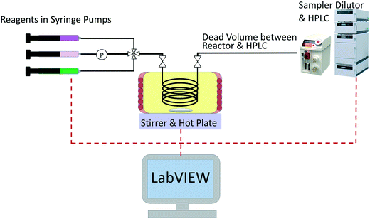Fig. 1 Simplified schematic of the experimental set-up used for transient experiments of the esterification of benzoic acid with ethanol using sulfuric acid as a homogenous catalyst.

Modelling a transient plug flow reactor

In the previous work, calculations demonstrated that the reactor behaved as an ideal PFR and thus the transient reactor was modelled using the mole balance for an ideal PFR as shown in eqn (6), where C_BA is the benzoic acid concentration (M), t is time (min), V is the reactor volume (L), ν is the volumetric flowrate (L min⁻¹) and r_BA (mol L⁻¹ min⁻¹) is the reaction rate.

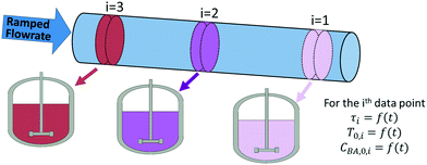
However in this work, to avoid solving partial differential equations which is often computational expensive, a hypothetical batch reactor approach was applied due to equivalence between the residence time in a PFR and the reaction time in a batch reactor.^12,16 The transient PFR can then be described by a system of ideal batch reactors, as demonstrated in Fig. 2, where each batch reactor is modelled using eqn (7) and (8), which are both ordinary differential equations. Here τ is the residence time (min) of the sample in the PFR which is equivalent to the reaction time of the hypothetical batch reactor. In this work all process variables are ramped from an initially high value downwards, therefore α_T is the rate of decrease in temperature (°C min⁻¹). This system of ordinary differential equations still maintains time dependence as the residence time of each hypothetical batch reactor, τ_i, and its initial conditions (temperature T_0,i and benzoic acid concentration C_BA,0,i) are functions of time, which is explained below and shown in eqn (9) to (12).

In eqn (7) and (8)N_sp is the overall number of sample data points.

Fig. 2 Plug flow reactor with ramped flowrate, modelled as a series of hypothetical batch reactors.

The initial temperature in the ith hypothetical batch reactor, T_0,i, is found from eqn (9), where T₀ is the initial temperature of the transient experiment, α_T is the temperature ramp rate and t_In,i is the time the ith sample entered the reactor (min). An equivalent equation for the initial benzoic acid concentration in the ith hypothetical batch reactor C_BA,0,i (M), is shown in eqn (10), where C_BA,0 is the initial benzoic acid concentration (M) in the transient experiment and α_C is the rate of decrease in concentration (M min⁻¹). The negative signs included in eqn (8)–(10), are because the flowrate, temperature and feed concentration were ramped from high initial values downwards at the given ramp rate of α_V, α_T or α_C.

T_0,i = T₀ − α_T × t_In,i (9)

C_BA,0,i = C_BA,0 − α_C × t_In,i (10)

For isothermal experiments, where only flowrate is ramped, a single transient experiment can be viewed as being equivalent to a single batch experiment. However, if temperature or feed concentration is simultaneously ramped with flowrate, then a single transient experiment is instead viewed as a collection of independent batch reactors which all have their own unique initial conditions and temperature profile (figures are shown in the ESI† for demonstration).

The time that each hypothetical batch reactor spent in the reaction zone, τ_i, (which is the equivalent reaction time for the corresponding batch reactor) is calculated according to eqn (11), as the difference between the times the sample entered, t_In,i (min) and left, t_L,i, (min) the reactor.

τ_i = t_L,i − t_In,i (11)

However, only the time at which the sample was measured by the HPLC, t_M,i, (min) is known for each data point, as recorded by the HPLC timestamp. This measurement time is different to the time that the sample left the reactor due to the section of tubing of dead volume V_d (44.2 μL) between the reactor outlet and the HPLC sample loop. For a PFR with a constantly ramped flowrate, the times the sample entered and left the reactor can be calculated using eqn (12), where v_o is the initial flowrate of the entire experiment (μL min⁻¹), α_V is the ramp rate at which flowrate is decreased (μL min⁻²) and V, the volume term (μL) is either replaced with the dead volume V_d, to calculate t_L,i, or replaced with the sum of the dead volume and reactor volume, V_d + V_r, to calculate t_In,i. Derivations for this equation can be found in the literature.^12,20

Modelling & parameter estimation

The reaction is modelled as a set of equations f, input variables u, state variables x, and a vector of N_θ non-measurable parameters θ which can be used to predict experimentally measurable values ŷ:

ŷ = f(x, u, θ) (13)

The model equations are the ideal batch reactor equations (eqn (7) and (8)) and the first-order rate law (eqn (2) and (3)). The input variables u, consist of both the fixed variables (sulfuric acid concentration) and the three control variables (temperature T, benzoic acid feed concentration C_BA,0, and flowrate ν), while the state variables x, are the reactant concentration along the length of the reactor. The measured variables y, are the outlet concentration of benzoic acid and ethyl benzoate and θ is a vector consisting of the two kinetic parameters KP1 and KP2. Parameter estimation is the process of using experimental measurements to estimate values for the non-measurable parameters θ. For an experimental data set that consists of N_exp experiments, each containing N_m measurements, then for the ith experiment and jth measurement the ij-th residual ρ_ij, is defined as the difference between the model predicted value ŷ_ij, and the experimentally measured value y_ij:

ρ_ij = y_ij − ŷ_ij for i = 1 to N_exp and for j = 1 to N_m (14)

In this work, the ith data point collected from a transient flow experiment, is equivalent to the ith batch reactor which can be viewed as the ith experiment in eqn (14). Parameter estimation was conducted using the maximum likelihood principle which assumes that i) the correct model structure is used ii) the experimental inputs u are perfectly controlled and iii) the residuals are caused by measurement errors σ_ij, which are normally distributed with a mean of 0 and a standard deviation σ_ij.^2,23 Parameter estimation is then an optimisation problem to find the optimum parameter values to maximise the log likelihood function Φ(θ) shown below:

The optimum parameter values, [small straight theta, Greek, circumflex], called the maximum likelihood estimates (MLE) were found by maximising eqn (15), the log likelihood function using the Nelder–Mead simplex algorithm in Python.²⁷ The solver requires an initial guess for the two kinetic parameters KP1 and KP2, which were assumed to be 9.12 (–) and 7.98 (J mol⁻¹) based on the results from previously published work.²⁰ After conducting parameter estimation, the adequacy of the model can be tested using the χ² test, where the χ² value is calculated using eqn (16) and compared to the reference value χ_ref² (N_expN_m − N_θ) computed from a χ² distribution with degrees of freedom N_expN_m – N_θ at 95% of significance.²³

If the χ² value is greater than the reference value, this is interpreted to mean that the model is not compatible with the experimental data and that the model should be rejected.

Due to randomly distributed experimental error, parameter estimates are themselves random variables with an associated precision or standard deviation. It is always desired to obtain parameter estimates with as high precision as possible (equivalent to low variance). The parameter precision is described by the N_θ × N_θ covariance matrix V_θ, which is calculated using the first order Taylor series approximation as shown in eqn (17).

V_θ ≅ H_θ⁻¹ (17)

where H_θ is the Fisher information matrix, which is calculated using the approximation shown below for the k, lth element of the Hessian, where the term is the sensitivity of the model prediction ŷ_ij with respect to the kth parameter.

From the covariance matrix V_θ, it is possible to compute an approximated confidence region for the parameter estimates in the form of a confidence ellipsoid with a given level of significance. In this work, 95% confidence ellipsoids are used to provide a visual quantification of the statistical quality of parameter estimates. Confidence ellipsoids are computed as the sets of parameters θ which satisfy the following equation

[θ − [small straight theta, Greek, circumflex]]^TV_θ⁻¹[θ − [small straight theta, Greek, circumflex]] ≤ χ_ref²(N_θ) (19)

where χ_ref²(N_θ) is the reference value computed from a χ² distribution with degrees of freedom N_θ at 95% of significance.

Model-based design of experiments

The design vector, φ, is defined as the vector which contains the experimental control variables that can be varied in the given experiment. MBDoE for improved parameter precision uses the information already known about a model to calculate the optimal values for the design vector to maximise the precision of model parameters. Normally, for designing transient experiments using MBDoE, the experimental duration is discretised into a number of regions, and in each time region every control variable is designed, most commonly using piecewise constant or piecewise linear method.²⁴ This creates a challenging MBDoE problem, as the design vector becomes very large, especially if many time intervals are used. The ramp transient experiments conducted in this work are a special case of the piecewise linear method, as instead of splitting the experimental duration into a number of different regions, only a single time region is used. The design vector then consists of only the initial value and a single ramp rate for each control variable. Therefore, this becomes an easier MBDoE problem to work with as it contains fewer degrees of freedom. In this case study, the design vector for a single experiment φ consists of up to 6 variables, i.e.φ = [T₀, α_T, v₀, α_V, C_BA,0, α_C]^T.

Mathematically MBDoE is based on two principles, the first being that it is possible to predict the expected Fisher information of any planned experiment, H_expected, using eqn (18) with some initial estimate for the parameter values θ, which can be obtained from the literature or from previously conducted experiments in the form of the MLE estimate [small straight theta, Greek, circumflex]. The second principle is the additivity of Fisher information which allows the expected covariance matrix V_θ,expected, after N_exp already completed experiments and N_new new planned experiments, to be calculated according to eqn (20).

where V_θ,0 is the prior covariance matrix obtained from the N_exp already conducted experiments and H_i,expected is the expected Fisher information obtained from the ith planned experiment. However, in this work MBDoE is conducted as if no prior experiments were conducted so the term V_θ,0 is removed from eqn (20).

The prior information used for experimental design is an initial guess for the parameter values KP1 and KP2, taken to be the values obtained from the previously published work of 9.12 (–) and 7.98 (J mol⁻¹).²⁰ It is worth highlighting that the initial guess for the parameter values from the previous work is considered quite good, which assists the MBDoE in designing the optimum experiment. Therefore, this is a case where the objective is to improve the precision of some initial estimates, similar to a situation where initial parameter estimates are obtained from the literature. In other situations where there is large uncertainty in the parameter values, MBDoE may lead to suboptimal designs. In these situations it may be more appropriate to use robust MBDoE techniques.^28–31 MBDoE designs for different initial guesses of the kinetic parameters are reported in the ESI,† where it is shown for this case study that while the design is influenced by the initial guess, the MBDoE designs with poor initial guess are still superior to intuitively designed experiments in terms of the precision of parameter estimates obtained.

MBDoE for improved parameter precision is an optimisation problem to find the optimum values for the design vector φ to minimise some scalar measure of the expected covariance matrix shown in eqn (20). In this work, the D-optimum criterion, which is the determinant of the expected covariance matrix, is used as the scalar measure of the covariance matrix²³ and hence the objective function ψ(φ,[small straight theta, Greek, circumflex]), is given by eqn (21).

This is a bounded optimisation problem, as the values for the design vector entries are constrained due to experimental limitations to the ranges shown in Table 1 and due to the three following additional experimental constraints.

Table 1 Allowable range of the elements in the design vector (initial flowrate v_o, flowrate ramp rate α_V, initial feed concentration C_BA,0, feed concentration ramp rate α_C, initial temperature T₀, temperature ramp rate α_T). Note that in all cases the values of flowrate, feed concentration and temperature are ramped downwards

Variable	v o (μL min^−1)	α V (μL min^−2)	C BA,0 (M)	α C (M min^−1)	T 0 (°C)	α T (°C min^−1)
Range	7.5–100	10^−5–1.25	0.9–1.55	10^−6–0.01	70–140	0–3

---

• The experimental duration is limited to a maximum of 100 min.

• The flowrate can never drop below 5 μL min⁻¹, as such a low flowrate would not adequately refill the HPLC sample loop between measurements leading to measurement errors.

• All variables must be ramped from an initial high value, downwards. For flowrate this is important, as before the transient experiment can begin the reactor must reach steady-state at the initial condition, so a fast initial flowrate minimises this initial waiting period.

The objective function ψ(φ) was minimised using the SLSQP (Sequential Least Squares Programming) algorithm in Python.³² This optimisation algorithm also needs an initial guess for the design vector φ, and in order to prevent the algorithm from getting stuck in a local optimum, 10 000 simulations were designed using a Latin hypercube within the allowed range of the design vector. This large number is chosen, as it guarantees a detailed coverage of the relatively small design space, which consists of only 3 variables. The expected covariance matrix for each of the 10 000 simulations was calculated and the design vector which produced the smallest determinant of the expected covariance matrix was used as the initial guess for the SLSQP algorithm. The optimised MBDoE design vector obtained from the SLSQP algorithm was then executed using the automated flow reactor platform.

Three different types of experimental scenarios were studied.

1. Ramp F, 2 experiments were designed where only flowrate was ramped while temperature and feed concentration were kept constant.

2. Ramp FT, 1 experiment was designed where both flowrate and temperature were ramped while feed concentration was kept constant.

3. Ramp FTC, 1 experiment was designed where temperature, flowrate and feed concentration were all ramped.

In all cases the MBDoE designs were compared against previously published experiments which were designed by researcher intuition, to try and explore as much of the design space as possible in a single experiment.²⁰ Note that for the Ramp FT and Ramp FTC scenarios, a single experiment was sufficient to estimate the kinetic parameters and therefore only 1 experiment was designed. The design vectors for these experiments consisted of 5 variables, φ^FT = [T₀, α_T, v₀, α_V, C_BA,0]^T and 6 variables, φ^FTC = [T₀, α_T, v₀, α_V, C_BA,0, α_C]^T. However, for the Ramp F scenario, two experiments conducted at different temperatures were required to estimate the kinetic parameters. Therefore the Ramp F MBDoE problem required the design of two experiments simultaneously resulting in a design vector with 8 variables φ^F = [T1₀, v1₀, α1_v, C1_BA,0, T2₀, v2₀, α2_v, C2_BA,0]^T.

Results & discussion

Design & execution of flowrate ramping experiments

The experimental designs for the two Ramp F experiments, designed by MBDoE in this work and designed intuitively in our previously published work,²⁰ are compared in Fig. 3a and b, and Table 2. Both MBDoE designs were found to have quite low flowrates, of less than 30 μL min⁻¹, which was surprising, as intuitively a wide range of flowrates would be considered preferable to allow the study of a wider range of residence times. In comparison in the previously published work the maximum initial flowrate of 100 μL min⁻¹ was decreased at a rate of 1 μL min⁻² for both experiments. The MBDoE designs also differed from the intuitively chosen designs in that both MBDoE experiments had the same inlet concentration of 1.55 M whereas the intuitive experiment designs ran one experiment at a low concentration and one at a high concentration. This shows the tendency of MBDoE designs to study a small section of the design space which carries the highest information, instead of studying a wide range of the design space.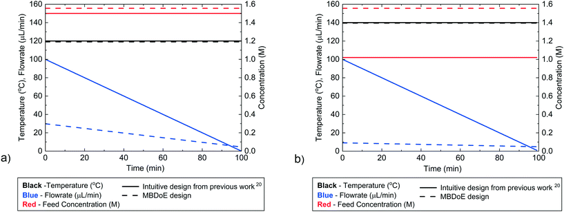

Fig. 3 Control variable profiles (temperature, flowrate and benzoic acid inlet concentration) designed by the intuitive method from previously published work²⁰ and by MBDoE for a) the first and b) the second Ramp F experiment.

Table 2 Flowrate ramping experiment designs showing the initial flowrate v_o, decreasing flowrate ramp rate α_V, benzoic acid feed concentration C_BA,0 and temperature T₀

Experiment	v o (μL min^−1)	α V (μL min^−2)	C BA,0 (M)	T 0 (°C)
Ramp F MBDoE 1	29.8	0.253	1.55	119.0
Ramp F MBDoE 2	9.13	0.043	1.55	139.4
Ramp F intuitive design 1^20	100	1.000	1.50	120.0
Ramp F intuitive design 2^20	100	1.000	1.02	140.0

---

The MBDoE designs in Table 2 were conducted using the automated flow reactor platform, and the reactor outlet concentrations measured by the HPLC are shown in the ESI.† The intuitive designs had already been conducted in the previously published work.²⁰ It was found that the MBDoE designed experiments led to significantly more precise estimates, as shown by the 95% confidence ellipsoid plot in Fig. 4 and the 95% confidence intervals reported in Table 3. However, when making this comparison it must be acknowledged that the superior design found by MBDoE required knowing the model structure and having an initial estimate of the parameter values in advance of conducting any experiments.

Fig. 4 95% confidence ellipsoids comparing the statistical certainty of the kinetic parameters KP1 and KP2 between the MBDoE and intuitive²⁰Ramp F experiments (see Table 2).

Table 3 Maximum likelihood estimates along with 95% confidence intervals for the parameter values KP1 and KP2, and the corresponding values of the Arrhenius parameters, k₀ and E_A, and χ² values for the Ramp F experiments (see Table 2)

Experiment	Experiment duration (h)	KP1 ± 95% CI (–)	KP2 ± 95% CI (J mol^−1)	k 0 × 10^−6 (s^−1)	E A (kJ mol^−1)	χ ^2/χref^2
Ramp F MBDoE	4	9.17 ± 0.10	8.18 ± 0.38	20.6	81.8	9.80/72.1
Ramp F intuitive design^20	4	9.03 ± 0.18	7.63 ± 0.76	4.15	76.3	25.9/67.5

---

Design & execution of simultaneous flowrate & temperature ramping experiments

For the Ramp FT experiments, where flowrate and temperature were ramped simultaneously, the intuitive and MBDoE experimental designs are compared in Fig. 5 and Table 4. It is observed that the MBDoE design is similar to the intuitive design for both the temperature profile and the constant feed concentration, however there is a large difference in the flowrate profiles. The intuitive design explored a wide range of flowrates, leading to a design with an initial flowrate of 100 μL min⁻¹ which was decreased at a rate of 1 μL min⁻². In contrast the MBDoE flowrate design only explored a small region of low flowrates, with the initial flowrate being only 10.1 μL min⁻¹ which was slowly decreased at a rate of just 0.05 μL min⁻².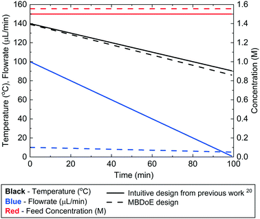

Fig. 5 Control variable profiles (temperature, flowrate and benzoic acid inlet concentration) designed by the intuitive method from previously published work²⁰ and by MBDoE for the Ramp FT experiments.

Table 4 Flowrate & temperature ramping experiment designs showing the initial flowrate v_o, decreasing flowrate ramp rate α_V, benzoic acid feed concentration C_BA,0, initial temperature T₀ and decreasing temperature ramp rate α_T

Experiment	v o (μL min^−1)	α V (μL min^−2)	C BA,0 (M)	T 0 (°C)	α T (°C min^−1)
Ramp FT MBDoE	10.1	0.05	1.55	139.2	0.537
Ramp FT intuitive design^20	100	1.00	1.50	140.0	0.500

---

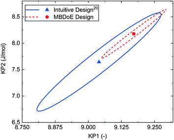
The MBDoE design was conducted using the automated reactor platform and the measured outlet concentrations are shown in the ESI.† The intuitive design had already been performed in the previously published work.²⁰ Despite some similarities in the experimental design, the MBDoE designed experiment was found to give much more precise parameter estimates than intuitive design, as shown in Fig. 6 by the smaller 95% confidence ellipsoid and in Table 5 by the smaller 95% confidence intervals. The large difference in the size of the confidence ellipsoids highlights how difficult it is to intuitively design a multi variate ramp transient experiment, and demonstrates the need for MBDoE approaches for their design.

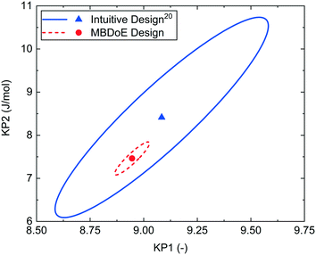Fig. 6 95% confidence ellipsoids comparing the statistical certainty of the kinetic parameters KP1 and KP2 between the MBDoE and intuitive²⁰Ramp FT experiments (see Table 4).

Table 5 Maximum likelihood estimates along with 95% confidence intervals for the parameter values KP1 and KP2, and the corresponding values of the Arrhenius parameters, k₀ and E_A, and χ² values for the Ramp FT experiments (see Table 4)

Experiment	Experiment duration (h)	KP1 ± 95% CI (–)	KP2 ± 95% CI (J mol^−1)	k 0 × 10^−6 (s^−1)	E A (kJ mol^−1)	χ ^2/χref^2
Ramp FT MBDoE	2	8.95 ± 0.07	7.46 ± 0.32	2.65	74.6	13.2/38.9
Ramp FT intuitive design^20	2	9.06 ± 0.40	8.36 ± 1.97	41.0	83.6	4.77/31.4

---

Table 6 Maximum likelihood estimates along with 95% confidence intervals for the parameter values KP1 and KP2, and the corresponding values of the Arrhenius parameters, k₀ and E_A. The χ² values for all experiments in this work and in previously published work²⁰ along with the approximate duration of each experiment are also shown

Experiment	Experiment duration (h)	KP1 ± 95% CI (–)	KP2 ± 95% CI (J mol^−1)	k 0 × 10^−6 (s^−1)	E A (kJ mol^−1)	χ ^2/χref^2
Ramp F MBDoE	4	9.17 ± 0.10	8.18 ± 0.38	20.6	81.8	9.80/72.1
Ramp F intuitive design^20	4	9.03 ± 0.18	7.63 ± 0.76	4.15	76.3	25.9/67.5
Ramp FT MBDoE	2	8.95 ± 0.07	7.46 ± 0.32	2.65	74.6	13.2/38.9
Ramp FT intuitive design^20	2	9.06 ± 0.40	8.36 ± 1.97	41.0	83.6	4.77/31.4
SS, factorial^20	8	9.11 ± 0.19	7.98 ± 0.77	11.7	79.8	0.98/23.7
SS, D Opt^20	8	9.17 ± 0.12	8.15 ± 0.46	18.8	81.5	10.6/23.7

---

Design of simultaneous flowrate, temperature & feed concentration ramping experiments

The final scenario was intended to ramp flowrate, temperature and inlet concentration, all simultaneously. However, the MBDoE algorithm designed an experiment where the initial inlet benzoic acid concentration was almost the maximum at 1.54 M, but the ramp rate in concentration was only 10⁻⁶ M min⁻¹, which was the lowest ramp rate allowed by the optimisation step. This resulted in an experiment where the concentration was practically constant (the proposed concentration varied from 1.54 to 1.5399 M). Therefore, it was concluded that ramping concentration offered no added value, as it was preferable to run at maximum concentration. It was considered that allowing concentration to be ramped in the MBDoE algorithm, just added an unnecessary extra design variable which made the optimisation more challenging. For these reasons the experiment was not conducted. This result is specific to this case study and it is expected that for other experimental systems ramping all three variables simultaneously may improve parameter estimates.

Comparison of parameter estimates from different experiments

In our previously published work,²⁰ the kinetics of benzoic acid and ethanol esterification using sulfuric acid as the catalyst was examined through a campaign of 8 steady-state experiments designed by the factorial method (SS factorial) and a separate campaign of 8 steady-state experiments designed by D-optimal MBDoE (SS MBDoE). In order to demonstrate that the parameter estimates from the previous work and the new transient experiments presented in this work are all consistent, 95% confidence plots of the parameter estimates from all experiments are shown in Fig. 7, where it can be observed that the confidence ellipsoids overlap. The only exception is the Ramp FT MBDoE designed transient experiment, whose confidence region overlaps with 3 of the experiments (Ramp F intuitive, Ramp FT intuitive and SS factorial) but does not overlap with the remaining 2 experiments (Ramp F MBDoE and SS MBDoE). The cause of this could be an unknown disturbance in the Ramp FT experiment or it could suggest that the modelling assumptions are wrong, for example that the measurement error is not randomly distributed with a mean of 0 and a constant standard deviation. However, as the parameter estimates are still very close this is not a major issue, nor does it undermine the result here which shows the considerable advantages of MBDoE design for transient experiments. Additionally, it is worth noting that the Ramp FT MBDoE designed experiment, where both temperature and flowrate were ramped simultaneously, produces one of the smallest confidence ellipsoids, comparable with the ellipsoid generated from the campaigns of 8 steady-state experiments designed using MBDoE. This demonstrates the value of MBDoE designed transient experiments, as the Ramp FT experiment which takes only 2 h, produces parameter estimates with similar levels of precision as experiments which take 4 h (Ramp F experiments) or 8 h (steady-state campaigns), provided that good initial guesses for the parameter values are available either from previous experiments or from values found in the literature.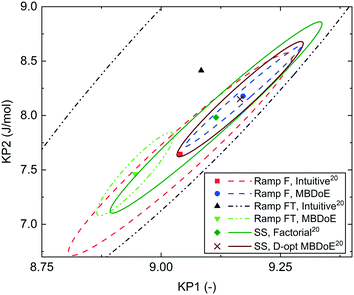

Fig. 7 95% confidence ellipsoids comparing the statistical certainty of the kinetic parameters KP1 and KP2 for different experiments performed in this work and previous work.²⁰ The kinetic parameters KP1 and KP2 are reparametrized forms of the Arrhenius activation energy and pre-exponential factor as shown in eqn (3). SS, Factorial is a campaign of 8 experiments designed by factorial methods, while SS, D-opt MBDoE is a campaign of 8 experiments designed by online D-optimal MBDoE.

When the reparametrised kinetic parameters KP1 and KP2 are converted back to the original Arrhenius constants of pre-exponential factor (k₀) and activation energy (E_A), the parameter estimates, which previously were all very similar in value, spread further apart. This is shown in Table 6 where the maximum and minimum pre-exponential factor estimates are 2.65 × 10⁶ s⁻¹ and 41.0 × 10⁶ s⁻¹, even though the reparametrised parameters were very similar in value at 8.95 and 9.06. This large difference in pre-exponential factor estimates is due to the exponential transformation between the two parametrisations and to the correlation between the pre-exponential factor and the activation energy, as higher pre-exponential factors are compensated by higher activation energies.

However, the important question is how well the kinetic parameter estimates can predict the reactor performance. Generally, the confidence in the model predictive capabilities should depend only on the confidence that the model structure is correct and the precision in parameter estimation. While the precision in parameter estimation can be calculated, unfortunately there is no good way to assess the confidence on the adequacy of the chosen model structure, as the model may be unable to represent all the phenomena taking place in the system. In order to test if the model predictions are accurate in a new area of the design space one needs to conduct experiments there, to ensure that there is not some new previously unknown reaction or phenomena occurring in the unexplored space. However, conducting experiments in unexplored areas of the design space as a method of model validation is a labour intensive effort. In most cases, if a model's parameters are estimated well and the model assumptions (model structure) are based on sound principles, there should be reasonable confidence that the model will perform well in unexplored regions, provided it is not extrapolated very far beyond the conditions for which it was developed. In this work the model's predictive performance was tested by using the parameter estimates obtained from the various experiments in both the current work and the previous work²⁰ to predict the transient experiments conducted in this work as shown in Fig. 8, and the steady-state experiments conducted in the previous work as shown in Fig. 9. The simulation predictions match closely the experimental measurements within the experimental error, even in cases where the predicted profiles were created using parameter estimates which were obtained from experimental data that explored a significantly different portion of the design space. In particular, it is worth noting that the kinetic parameter estimates obtained from transient experiments are able to predict steady-state reactor behaviour and vice versa.

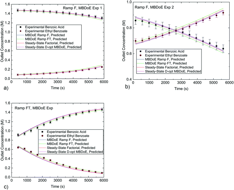Fig. 8 Experimental concentrations from the MBDoE designed transient experiments conducted in this work compared against predicted values using parameter estimates obtained from different experiments in this work and previously published work.²⁰ a) and b) are for the Ramp F MBDoE designed experiments, c) is for the Ramp FT MBDoE designed experiment. Error bars indicate 1 standard deviation of the experimental measurement error which was 0.030 M for benzoic acid and 0.0165 M for ethyl benzoate.

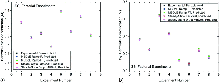Fig. 9 Experimental concentrations of a) benzoic acid and b) ethyl benzoate obtained from the steady-state factorial experiments conducted in previous work²⁰ compared against predicted values using parameter estimates obtained from the MBDoE Ramp F, MBDoE Ramp FT, Steady-State Factorial and Steady-State D-opt MBDoE experiments. Error bars represent 1 standard deviation of the experimental measurement error which was 0.030 M for benzoic acid and 0.0165 M for ethyl benzoate.

Concluding remarks

In this work, it is shown that MBDoE provides a useful tool to design single and multi-variable ramp transient experiments to estimate kinetic parameters precisely. This is particularly valuable as these designs are non-intuitive. For the case study considered, the esterification of benzoic acid with ethanol, the optimum design of all transient experiments conducted suggested to use low initial flowrates which were slowly ramped down over the course of the experiment. This design resulted in experiments investigating narrow ranges of residence times and demonstrates that the optimum experiment for parameter precision focuses on repeatedly sampling the design space in a narrow high information zone rather than sampling a wide range of different experimental conditions which carry less information, but which may be useful for model validation. The parameter precision obtained by model-based design of transient experiments was very similar to that obtained from campaigns of steady-state experiments, despite the transient experiments requiring significantly less time and resources to run. This highlights the potential for model-based designed transient experiments to improve the efficiency of kinetic studies.

While transient experiments were found to be very effective for this case study, it is important to highlight that they can only be applied to systems which exhibit near instantaneous response to changes in the process conditions. Some catalysts, such as Fischer–Tropsch catalysts, have an induction time for the catalyst to come into equilibrium with changing process conditions.¹⁴ If this induction time is significant compared to the ramp rate of the experiment, transient methods would lead to erroneous results. However, there are many catalysts which do exhibit fast responses to changing process conditions, such as oxidation of carbon monoxide and steam reforming of methanol both of which were successfully studied using temperature ramped transient experiments.¹⁵ Therefore, the application of transient experiments is most suited to non-catalytic reactions and systems with catalysts that are stable (or very slowly deactivating) and equilibrate sufficiently quickly with their environment. From the experimental point of view, satisfactory closure of the carbon balance, well-controlled ramps of the control variables, well-characterised reactor and system hydrodynamic behaviour (e.g. PFR behaviour, no dead volumes between reactor outlet and sampling) are important to provide accurate results.

A limitation to keep in mind for this experimental design technique is that, like all model-based methods, it is necessary to assume a suitable model structure in advance along with some initial estimates for all the model parameters. In most cases it is possible to make such assumptions based on information from the literature or researcher experience with similar reactions. If MBDoE is applied with an incorrect model structure or particularly poor parameter estimates, there is no guarantee that that the designed experiment will provide highly informative data, although similarly there is no guarantee that an intuitive design will provide highly informative data either. Generally, if there is high confidence in the model structure, but low confidence in the parameter estimates, it is still advised to use MBDoE for improved parameter precision to design a sequence of transient experiments. This strategy benefits from the fact that as each experiment is conducted, the parameter estimates become more precise, so that the following MBDoE design becomes more effective. Furthermore, in the event of low confidence in the parameter estimates, robust MBDoE techniques could be used.^28–31 If however, there is low confidence in the model structure, MBDoE for improved parameter precision should not be used. If there is low confidence in the model because there are two or more candidate models available, transient experiments could be designed using MBDoE for model discrimination. Alternatively, if there is no suitable model structure available, the best option is to use traditionally designed transient experiments to span as much of the design space as possible. This can be used as a starting point to collect kinetic data, before proposing new candidate models and eventually being able to use the more efficient MBDoE techniques for transient experiment design.

Conflicts of interest

The authors have no conflicts of interest to declare.

Acknowledgements

C. Waldron and A. Pankajakshan thank the department of Chemical Engineering in University College London for their PhD studentships, and M. Quaglio thanks the Hugh Walter Stern PhD Scholarship, University College London for his funding.

References

1. D. G. Blackmond, J. Am. Chem. Soc., 2015, 137, 10852–10866.
2. G. Franceschini and S. Macchietto, Chem. Eng. Sci., 2008, 63, 4846–4872.
3. O. P. Schmidt, A. M. Dechert-Schmitt, M. R. Garnsey, H. M. Wisniewska and D. G. Blackmond, ChemCatChem, 2019, 11, 3808–3813.
4. D. G. Blackmond, Angew. Chem., Int. Ed., 2005, 44, 4302–4320.
5. N. Al-Rifai, E. Cao, V. Dua and A. Gavriilidis, Curr. Opin. Chem. Eng., 2013, 2, 338–345.
6. T. Salmi, J. Hernández Carucci, M. Roche, K. Eränen, J. Wärnå and D. Murzin, Chem. Eng. Sci., 2013, 87, 306–314.
7. S. Tadepalli and A. Lawal, Curr. Opin. Chem. Eng., 2009, 6, 1542–6580.
8. J. Zhang, Y. Lu, Q. Jin, K. Wang and G. Luo, Chem. Eng. J., 2012, 203, 142–147.
9. J. P. McMullen and K. F. Jensen, Org. Process Res. Dev., 2011, 15, 398–407.
10. B. J. Reizman and K. F. Jensen, Org. Process Res. Dev., 2012, 16, 1770–1782.
11. J. S. Moore and K. F. Jensen, Angew. Chem., Int. Ed., 2014, 53, 470–473.
12. C. A. Hone, N. Holmes, G. R. Akien, R. A. Bourne and F. L. Muller, React. Chem. Eng., 2017, 2, 103–108.
13. C. A. Hone, A. Boyd, A. O'Kearney-McMullan, R. A. Bourne and F. L. Muller, React. Chem. Eng., 2019, 4, 1565–1570.
14. B. Wojciechowski, Catal. Today, 1997, 36, 167–190.
15. B. Wojciechowski, Chem. Eng. Commun., 2003, 190, 1115–1131.
16. K. C. Aroh and K. F. Jensen, React. Chem. Eng., 2018, 3, 94–101.
17. B. M. Wyvratt, J. P. McMullen and S. T. Grosser, React. Chem. Eng., 2019, 4, 1637–1645.
18. S. Mozharov, A. Nordon, D. Littlejohn, C. Wiles, P. Watts, P. Dallin and J. M. Girkin, J. Am. Chem. Soc., 2011, 133, 3601–3608.
19. S. Schwolow, F. Braun, M. Rädle, N. Kockmann and T. Röder, Org. Process Res. Dev., 2015, 19, 1286–1292.
20. C. Waldron, A. Pankajakshan, M. Quaglio, E. Cao, F. Galvanin and A. Gavriilidis, React. Chem. Eng., 2019, 4, 1623–1636.
21. J. S. Moore, C. D. Smith and K. F. Jensen, React. Chem. Eng., 2016, 1, 272–279.
22. G. Buzzi-Ferraris and P. Forzatti, Chem. Eng. Sci., 1983, 38, 225–232.
23. Y. Bard, Nonlinear Parameter Estimation, Academic Press, New York, 1974.
24. S. Asprey and S. Macchietto, Comput. Chem. Eng., 2000, 24, 1261–1267.
25. M. Quaglio, C. Waldron, A. Pankajakshan, E. Cao, A. Gavriilidis, E. S. Fraga and F. Galvanin, Comput. Chem. Eng., 2019, 124, 270–284.
26. S. D. Schaber, S. C. Born, K. F. Jensen and P. I. Barton, Org. Process Res. Dev., 2014, 18, 1461–1467.
27. J. A. Nelder and R. Mead, Comput. J., 1965, 7, 308–313.
28. H. Dette, I. M. Lopez, I. M. O. Rodriguez and A. Pepelyshev, J. Stat. Plan. Inference, 2006, 136, 4397–4418.
29. H. Dette, V. B. Melas, A. Pepelyshev and N. Strigul, J. Theor. Biol., 2005, 234, 537–550.
30. S. Asprey and S. Macchietto, J. Process Control, 2002, 12, 545–556.
31. S. Körkel, E. Kostina, H. G. Bock and J. P. Schlöder, Optim. Methods Softw., 2004, 19, 327–338.
32. E. Jones, T. Oliphant and P. Peterson, SciPy:Open Source Scientific Tools for Python, http://www.scipy.org/.

---

Footnote

† Electronic supplementary information (ESI) available. See DOI: 10.1039/c9re00342h

---