
 Open Access Article
 This Open Access Article is licensed under a Creative Commons Attribution-Non Commercial 3.0 Unported Licence
Effect of Bi-substitution into the A-site of multiferroic La0.8Ca0.2FeO3 on structural, electrical and dielectric properties
H. Issaoui*ab,
A. Benalibc,
M. Bejarb,
E. Dhahrib,
B. F. O. Costaa,
M. P. F. Gracac and
M. A. Valentec
aCFisUC, Physics Department, University of Coimbra, P-3004-516 Coimbra, Portugal. E-mail: hajerissawui@yahoo.fr
bLaboratoire de Physique Appliquée, Faculté des Sciences, Université de Sfax, B.P. 1171, 3000 Sfax, Tunisia
cI3N and Physics Department, University of Aveiro, Aveiro, 3810-193, Portugal
First published on 23rd April 2020
Abstract
(La0.8Ca0.2)1−xBixFeO3 (x = 0.00, 0.05, 0.10, 0.15 and 0.20) (LCBFO) multiferroic compounds have been prepared by the sol–gel method and calcined at 800 °C. X-ray diffraction results have shown that all samples crystallise in the orthorhombic structure with the Pnma space group. Electrical and dielectric characterizations of the synthesized materials have been performed using complex impedance spectroscopy techniques in the frequency range from 100 Hz to 1 MHz and in a temperature range from 170 to 300 K. The ac-conductivity spectra have been analysed using Jonscher's power law σ(ω) = σdc + Aωs, where the power law exponent (s) increases with the temperature. The imaginary part of the complex impedance (Z′′) was found to be frequency dependent and shows relaxation peaks that move towards higher frequencies with the increase of the temperature. The relaxation activation energy deduced from the Z′′ vs. frequency plots was similar to the conduction activation energy obtained from the conductivity. Hence, the relaxation process and the conduction mechanism may be attributed to the same type of charge carriers. The Nyquist plots (Z′′ vs. Z′) at different temperatures revealed the appearance of two semi-circular arcs corresponding to grain and grain boundary contributions.
1 Introduction
Perovskite-type ferrites with the general formula AFeO3 are among the most promising materials in several fields of application. Recently, they have been used for fuel cells, sensors, magnetic memories, spintronic devices, etc.1–5 In addition, great attention has been paid to the iron oxide LaFeO3 (LFO) due to its excellent properties and use for technological applications, such as in transducers with magnetic modulation,6 fuel cells,7 catalysts,8 chemical sensors,9,10 magnetic materials11,12 and oxygen permeation membranes.13,14However, more recent studies have been conducted on doped iron oxides, such as La1−xCaxFeO3, due to their fascinating magnetic and electrical properties.15,16 These compounds have a transition from ferromagnetic (FM) to paramagnetic (PM) state at TC = 670 K.17 The iron-based perovskite derivatives of general formula La1−xAxFe1−yByO3 (A = Ba, Ca, Pb, Sr,…/B = Cr, Sm, Nb,…) have been widely studied by combining the effects of substitution and of the preparation method to improve the dielectric, ferromagnetic and ferroelectric properties.18–20
In addition, these materials have a giant dielectric constant and a low dielectric loss around room temperature.19 Materials with such properties have been used mainly in the manufacture of electronic devices, in particular such as capacitors and dynamic random access memories known as DRAM.21
Note here that the substitution of lanthanum ions by those of calcium has the effect of reducing electrical resistance and improving magnetic and dielectric properties, which allows the use of these materials La1−xCaxFeO3 (LCFO) as gas sensors and as a cathode in solid oxide fuel cells (SOFC).22–25
In our previous study, we have proved that the relaxation process in La0.8Ca0.2FeO3 compound prepared is of polaronic type, which is caused by the jumps of the charge carriers between the different iron ions.26 The NSPT model (small polaron without overlapping tunnel effect) has been used to study the conduction mechanism of the La0.8Ca0.2FeO3 compound. We also confirmed a huge dielectric constant with low dielectric loss tangent for the (La0.8Ca0.2)0.9Bi0.1FeO3 compound.27 This later also presented two relaxation processes, which are associated to grains and boundary grains contributions. This compound has been annealed at 800 °C as the series of samples we present in the present study.
In previous works we studied several properties of the (La0.8Ca0.2)1−xBixFeO3 (x ≤ 0.20) series annealed at different temperatures.28,29 We chose to do a more detailed study, namely on electrical and dielectrical properties, on the series annealed at 800 °C as the grain size of the samples is smaller in this series.
In this study, we focus on the synthesis and study of the effect of insertion bismuth ions in A-site of (La0.8Ca0.2)1−xBixFeO3 (with x = 0.00, 0.05, 0.10, 0.15 and 0.20).
2 Experimental techniques
The nanosized crystalline (La0.8Ca0.2)1−xBixFeO3 (x = 0.00, 0.05, 0.10, 0.15 and 0.20) LCBFO compounds have been prepared by the sol–gel method30 using as raw precursors lanthanum nitrate, bismuth nitrate, calcium nitrate, ferric nitrate and citrate acid (all analytically pure).| 0.8(1 − x)La(NO3)3 + 0.2(1 − x)Ca(NO3)2 + xBi(NO3)2 + Fe(NO3)3 → (La0.8Ca0.2)1−xBixFeO3 |
First, the precursors were mixed in distilled water. Afterwards, citric acid and ethylene glycol were added with constant stirring at room temperature for 5 h, in order to improve the consistency and the consequent formation of the gel. The mixture obtained was then heated to 170 °C until the formation of a black powder. This powder was pressed into thin pellets about 12 mm in diameter and ca. 1.5 mm thick and subjected to heat treatments at different temperatures (400 and 600 °C for 12 hours, 700 °C for 24 hours), interrupted by grinding cycles. Finally, the powders obtained were calcined at 800 °C (LCBFO800) for 72 hours.30 The phase purity, homogeneity, lattice structure and cell parameters of the synthesized compounds have been checked out by X-ray diffraction (XRD) analysis, using a Bruker 8D Advance X-ray powder diffractometer, with Cu Kα1 radiation (λ = 1.5406 Å), in θ–2θ Bragg–Brentano geometry. The acquisition has been chosen to be in the 2θ range of 5–100°, with a step of 0.02° and an acquisition time for each step of 1 s. The XRD data have been also used to obtain the lattice parameters by means of Rietveld analysis,31 using the FullProf program.
For the electrical measurements, a system formed by a vertical electric furnace and a dry rotary pump, in a closed cycle setup, connected to the extremes of the furnace has been used. This non-inductive electrical furnace operates from room temperature up to 1473 K. In each measurement, the sample has been mechanically pressed between two parallel platinum plates, forming the electrodes. The ac impedance of the samples has been measured between 170 and 300 K, and in the frequency range of 100 Hz up to 1 MHz, using an Agilent 4294A Precision Impedance Analyzer.
3 Results and discussion
3.1 Structural properties
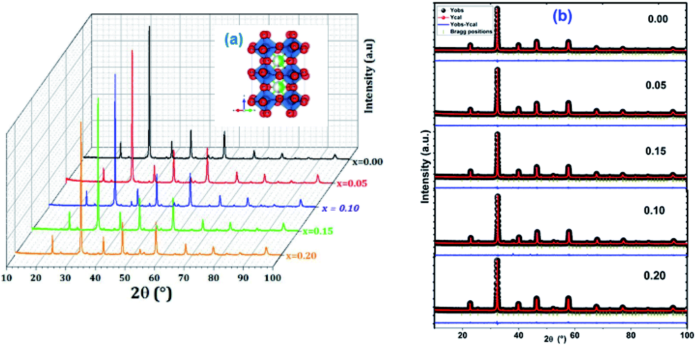 | ||
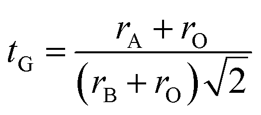
| Fig. 1 (a) Room temperature XRD patterns for (La0.8Ca0.2)1−xBixFeO3 (x = 0.00, 0.05, 0.10, 0.15 and 0.20) compounds. (b) The FullProf refined XRD; observed (red circle), calculated (black continuous line) and difference patterns (blue line) of X-ray diffraction data. The vertical tick indicates the Bragg positions. The inset exhibits the crystal structure. | ||
| x | 0.00 | 0.05 | 0.10 | 0.15 | 0.20 |
| Space group | Pnma | ||||
| 〈rA〉 (Å) | 1.208 | 1.199 | 1.190 | 1.181 | 1.173 |
| Tolerance factors (t) | 0.912 | 0.909 | 0.905 | 0.902 | 0.899 |
| a (Å) | 5.524 | 5.526 | 5.528 | 5.533 | 5.539 |
| b (Å) | 7.808 | 7.809 | 7.812 | 7.813 | 7.822 |
| c (Å) | 5.527 | 5.525 | 5.528 | 5.526 | 5.530 |
| Unit cell volume V (Å3) | 59.609 | 59.607 | 59.695 | 59.734 | 59.907 |
| Fe–O1 | 1.991 | 1.987 | 1.964 | 1.988 | 1.990 |
| Fe–O2 | 2.013 | 2.002 | 2.111 | 1.997 | 1.999 |
| Fe–O2 | 1.972 | 1.982 | 1.940 | 1.985 | 1.9870 |
| 〈Fe–O〉 | 1.992 | 1.990 | 2.005 | 1.990 | 1.992 |
| Fe–O1–Fe | 157.420 | 158.430 | 159.748 | 158.571 | 158.576 |
| Fe–O2–Fe | 158.210 | 158.190 | 151.611 | 158.174 | 158.174 |
| 〈Fe–O–Fe〉 | 157.815 | 158.310 | 155.679 | 158.372 | 158.375 |
| χ2 | 1.251 | 1.280 | 2.435 | 1.245 | 1.264 |
| Rp | 10.8 | 10.2 | 14.5 | 15.5 | 12.0 |
| Rwp | 12.2 | 10.7 | 15.8 | 16.5 | 11.8 |
| Re | 10.9 | 9.43 | 10.1 | 14.8 | 10.5 |
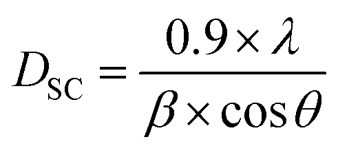
In order to confirm the structure of materials, Goldschmidt has defined a tolerance factor tG which provides information on the stability and distortion of the crystal structure using geometric criteria:32
The arithmetic values of the ionic rays of ions occupying sites A, B and O respectively are calculated as follows:
| 〈rO〉 = rO2− |
| 〈rB〉 = rFe3+ |
| 〈rA〉 = 0.8(1 − x)rLa3+ + 0.2(1 − x)rCa2+ + xrBi3+ |
The calculated tolerance factor values are grouped in the Table 1. According to this table, it can be seen that the tG values decrease with the increase of bismuth rate due to a decrease in the average ionic radius of the site A. The decrease in the tolerance factor tG bring about the system to the most symmetrical structure. Based on the Tokura et al. study,33 we can deduce that our LCBFO compounds show an orthorhombic agreement.
Concerning the method of Debye–Scherer,34 the expressed as follows:
 | (1) |
For the Williamson–Hall method, the widening of the X-ray line (β) equal to the expansion caused by the deformation of the lattice (βstrain) present in the material35 plus the contribution of crystallite size (βsize).
| β = βstrain + βsize | (2) |
![[thin space (1/6-em)]](https://www.rsc.org/images/entities/char_2009.gif) tanθ: with ε is a coefficient related to strain effect on the crystallites and
tanθ: with ε is a coefficient related to strain effect on the crystallites and 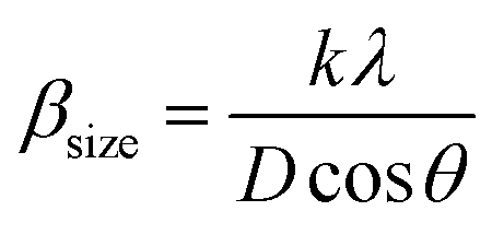 : from Scherer's formula
 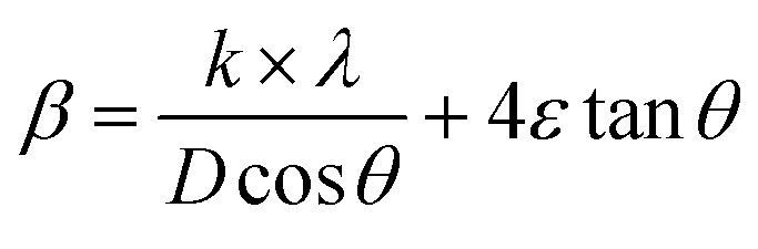 .
.
Therefore, (eqn (2)) becomes: 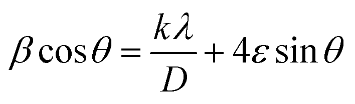 .
.
Afterwards, by the representation of βcosθ = f(4sinθ) (Fig. 2), we can determine the crystallite size DWH and the microstrain, respectively, from the intercept of the line at x = 0 and from the slope of the linearly fitted data. The obtained values for the crystallite sizes DSC and DWH and for the microstrain ε are summarized in Table 2.
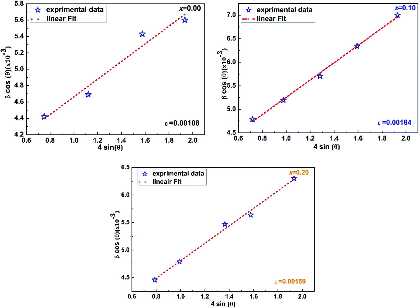 | ||
| Fig. 2 Williamson–Hall plot of (La0.8Ca0.2)1−xBixFeO3 (x = 0.00, 0.10, and 0.20) compounds. | ||
| x | 0.00 | 0.05 | 0.10 | 0.15 | 0.20 |
| DSC (nm) | 33.60 | 34.64 | 36.47 | 37.42 | 37.61 |
| DWH (nm) | 38.82 | 40.06 | 41.05 | 42.56 | 43.07 |
| ε (%) | 0.108 | 0.125 | 0.184 | 0.149 | 0.159 |
Fig. 3 shows the variation of the average size of the crystallites as a function of the bismuth level calculated by the two methods for the LCBFO compounds.
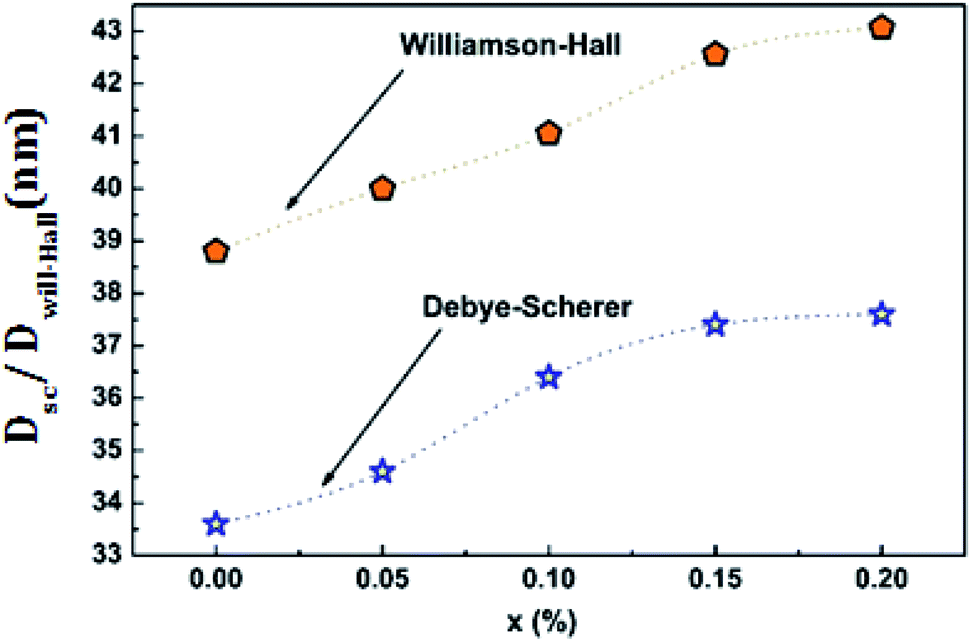 | ||
| Fig. 3 Variation of the average size for the crystallites as a function of the bismuth rate calculated by the two methods of Debye–Scherer and Williamson–Hall for (La0.8Ca0.2)1−xBixFeO3 (x = 0.00, 0.05, 0.10, 0.15 and 0.20) compounds. | ||
From Table 2 and Fig. 3, we can confirm the nanometric size of the crystallites. It is worth noting that the crystallite size calculated by Debye–Scherrer technique is slightly lower than that calculated by Williamson–Hall method because the broadening effect due to the microstrains completely excluded in Debye–Scherrer technique.
Also, we note a small increase in the size of the crystallites by increasing the bismuth rate. This increase is proportional previously detected for the volume.
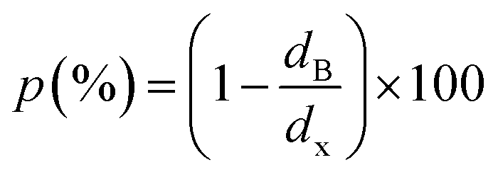 | (3) |
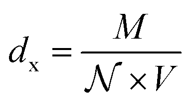 | (4) |
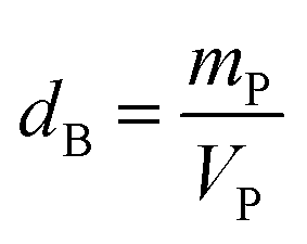 | (5) |
 is the Avogadro number, V the volume determined from the XR results, mP is the mass of the pellet and VP is the volume of the pellet.
The values of the density of XR (dx), the apparent density (dB) and the porosity (p) are summarized in the Table 3. According to this table, we note an increase in the porosity with the increase in the rate of bismuth. On the other hand, our (p) values are found to be very similar to those mentioned by N. Rezlescu et al.37 and Q. Rong et al.38 for such an application (gas sensors).
| x | 0.00 | 0.05 | 0.10 | 0.15 | 0.20 |
| dB (g cm−3) | 3.343 | ||||
| dx (g cm−3) | 6.218 | 6.357 | 6.483 | 6.627 | 6.755 |
| p (%) | 46.226 | 47.404 | 48.444 | 49.547 | 50.500 |
3.2 Morphological study
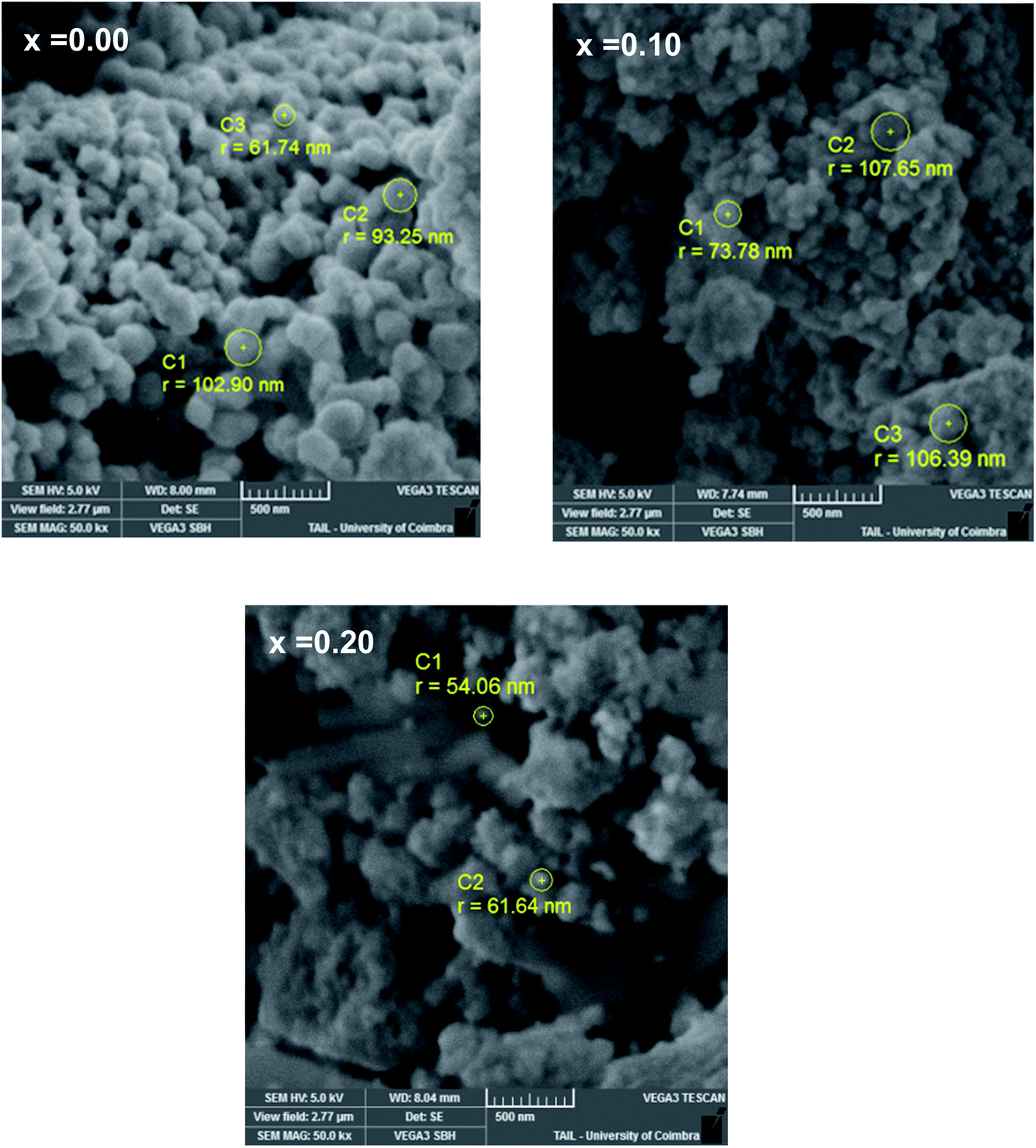 | ||
| Fig. 4 SEM micrographs of (La0.8Ca0.2)1−xBixFeO3 (x = 0.00, 0.10, and 0.20) compounds. | ||
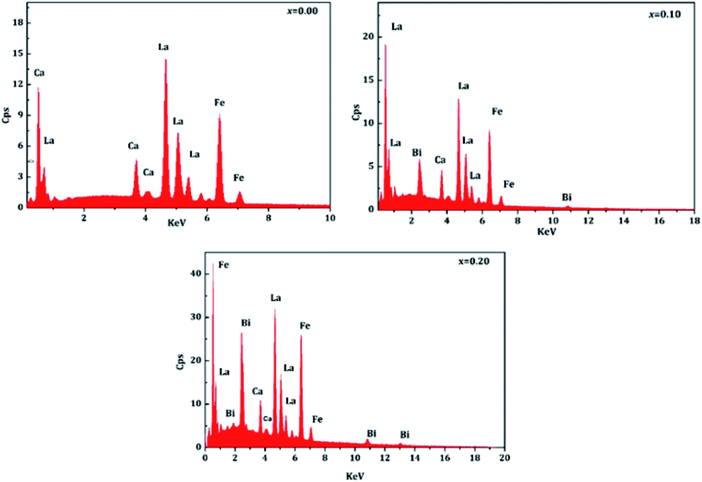 | ||
| Fig. 5 EDS spectra of (La0.8Ca0.2)1−xBixFeO3 (x = 0.00, 0.10 and 0.20) compounds. | ||
The elementary compositions in terms of atomic percentages and percentages by weight are shown in the Table 4. These values are almost in agreement with the stoichiometry of the starting materials used for the preparation of samples.
| Element | Weight (%) | Atomic (%) |
|---|---|---|
| x = 0.00 | ||
| Oxygen | 22.5 (7.4) | 58.1 |
| Calcium | 3.7 (0.4) | 4.3 |
| Iron | 25.6 (2.0) | 20.9 |
| Lanthanum | 48.2 (3.7) | 16.7 |
|
||
| x = 0.05 | ||
| Oxygen | 29.7 (9.1) | 69.6 |
| Calcium | 3.3 (0.4) | 3.2 |
| Iron | 23.1 (1.7) | 15.6 |
| Lanthanum | 40.8 (3.1) | 11.0 |
| Bismuth | 3.1 (0.5) | 0.6 |
|
||
| x = 0.10 | ||
| Oxygen | 23.4 (8.3) | 71.6 |
| Calcium | 3.5 (0.4) | 2.8 |
| Iron | 24.3 (1.9) | 14.7 |
| Lanthanum | 41.2 (3.4) | 9.7 |
| Bismuth | 7.7 (0.8) | 1.2 |
|
||
| x = 0.15 | ||
| Oxygen | 25.5 (7.5) | 66.1 |
| Calcium | 3.0 (0.3) | 3.1 |
| Iron | 23.8 (1.7) | 17.7 |
| Lanthanum | 36.6 (2.6) | 11.0 |
| Bismuth | 11.1 (1.1) | 2.2 |
|
||
| x = 0.20 | ||
| Oxygen | 24.7 (7.9) | 65.0 |
| Calcium | 3.1 (0.3) | 3.3 |
| Iron | 23.5 (1.7) | 18.1 |
| Lanthanum | 34.5 (2.5) | 10.7 |
| Bismuth | 14.2 (1.3) | 2.9 |
4 Dielectric and electrical studies
4.1 Complex impedance spectrum
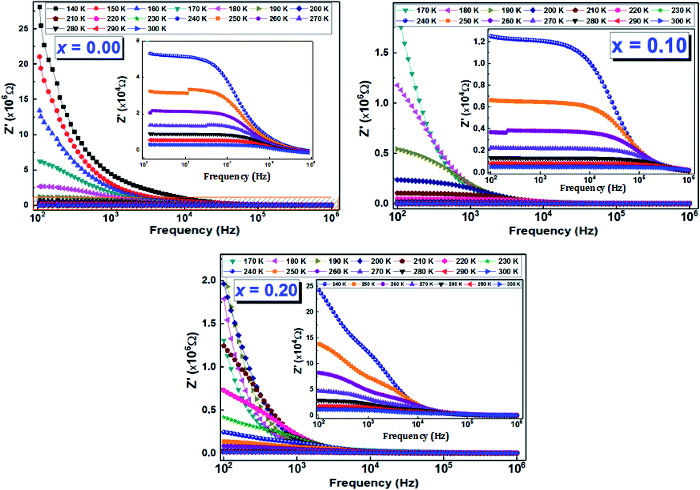 | ||
| Fig. 6 The frequency dependence of the real part of the complex electrical impedance (Z′) at several temperatures of (La0.8Ca0.2)1−xBixFeO3 (x = 0.00, 0.10, and 0.20) compounds. | ||
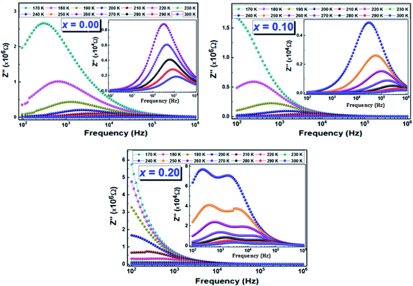 | ||
| Fig. 7 The frequency dependence of the imaginary part of the complex electrical impedance (Z′′) at several temperatures of (La0.8Ca0.2)1−xBixFeO3 (x = 0.00, 0.10, and 0.20) compounds. | ||
In addition, for all compounds, the relaxation peaks move towards the high frequencies when we increase the temperature, which indicates that the relaxations are thermally activated.44
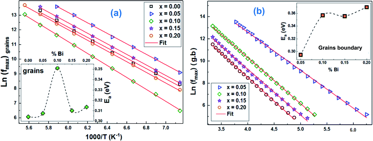
Using the frequency positions of these peaks (fmax), we have calculated the activation energies for the two contributions. The logarithmic variations of the frequencies corresponding to the relaxations ln(fmax) as a function of the temperature inverse (1/T) of the LCBFO compounds are shown in Fig. 8. We note that, for all the compounds and for the both contributions, this variation leads to linear behaviour with a slope, which varies according to the rate of substitution. This means that the relaxations perfectly follow the Arrhenius law given by the following equation:
 | (6) |
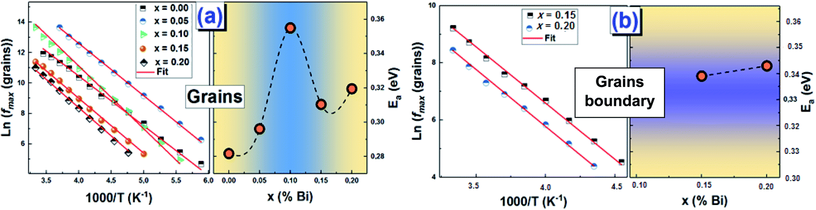 | ||
| Fig. 8 Variation of ln(fmax (Z′′)) as a function of 1000/T and the activation energies corresponding to (a) gains and (b) grain boundaries of (La0.8Ca0.2)1−xBixFeO3 (x = 0.00, 0.05, 0.10, 0.15 and 0.20) compounds. | ||
From the activation energy values (Fig. 8), we can note that the activation energy relative to the relaxation of the grains shows an increasing tendency with substitution and that it reaches a maximum value for the compound with 10% of bismuth then decreases for further bismuth concentrations. This decrease may be due to the increase in the charge carriers during the increase in the Bi-content.
According to literature, when the relaxation activation energy of such material is in the range between 0.2 and 0.4 eV, the relaxation process is known to be polaronic with a jump between B-site ions states.45,46 Accordingly, we deduce that the polaronic nature of the relaxation processes in the studied compounds.
The Nyquist diagrams relating to our LCBFO compounds, which are obtained at different temperatures, are shown in Fig. 9. All diagrams are made up of two arcs of circles located below the real axis; the first one is observed at high frequencies while the second arc of circle, having a larger radius, is observed at low frequencies. This second arc is associated to the grain boundaries resistance (RGB) contribution, while the first one represents the grains contribution.48 We also note that, for all LCBFO compounds, the radii of the half-arcs decrease while increasing the temperature, which proves the increase in electrical conductivity with temperature.49
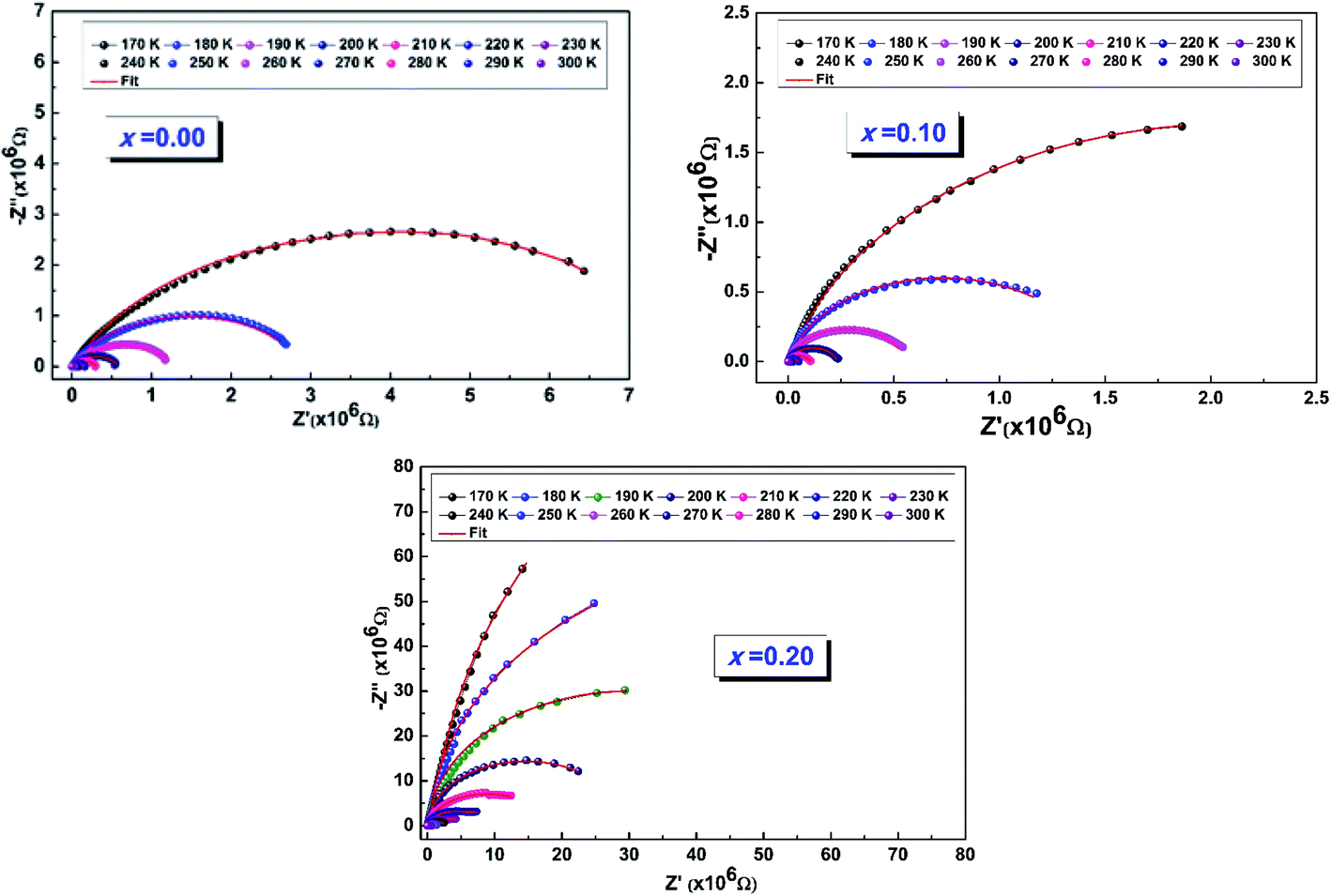 | ||
| Fig. 9 The fit of the experimental data using this equivalent circuit of Fig. 10. | ||
Given the existence of two arcs, the adjustment of Nyquist diagrams must be done with an equivalent circuit containing two sub-circuits connected in series.
We performed the modeling with Z-View software,50 and the best fit is obtained using an equivalent electrical circuit consisting of a series combination of two contributions. The first contribution corresponds to grain boundaries (RGB–CPEGB) (with CPE is the fractal impedance capacity) and the second is associated with grains (RG–CG), as shown in Fig. 10.
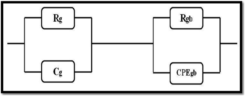 | ||
| Fig. 10 The equivalent circuit formed by a parallel combination of grain resistance. (RG–CG circuit) and constant phase element impedance (ZCPE) (RGB–CPEGB circuit). | ||
The resistance and capacitance values of the two contributions, for all the compounds, resulting from the adjustment with the Z-View software using the circuit mentioned above, are tabulated in Table 5. We note, from this table, that the resistance of the two contributions decreases with temperature, which confirms the semiconductor behaviour of all the LCBFO compounds.51 On the other hand, we can clearly see that for all compounds, the resistance of grain boundaries (RGB) is greater than that of grains (RG). This can be attributed to the fact that the atomic arrangement near the region of the grain boundaries is disordered, resulting in increased electron scattering. The logarithmic variations of the resistances RG and RGB as a function of the temperature inverse for our compounds are illustrated in Fig. 11(a) and (b). The activation energies are determined from Arrhenius' law:
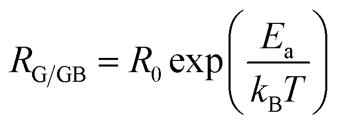 | (7) |
| T (K) | RJG (×105 Ω) | CPEJG (×10−9 F) | α | RG (×103 Ω) | CG (×10−10 F) |
|---|---|---|---|---|---|
| x = 0.00 | |||||
| 170 | 76.60 | 0.43 | 0.75 | 1.85 | 0.24 |
| 180 | 37.65 | 0.64 | 0.74 | 1.32 | 3.90 |
| 190 | 21.28 | 1.06 | 0.73 | 0.84 | 3.70 |
| 200 | 9.86 | 1.31 | 0.76 | 0.51 | 2.50 |
| 210 | 5.30 | 1.71 | 0.74 | 0.31 | 2.18 |
| 220 | 3.30 | 2.13 | 0.75 | 0.21 | 1.90 |
| 230 | 2.01 | 2.36 | 0.76 | 0.15 | 1.67 |
| 240 | 1.19 | 2.30 | 0.78 | 0.10 | 1.50 |
| 250 | 0.67 | 1.62 | 0.82 | 0.07 | 1.24 |
| 260 | 0.43 | 1.89 | 0.82 | 0.06 | 1.37 |
| 270 | 0.26 | 1.25 | 0.87 | 0.04 | 1.28 |
| 280 | 0.18 | 1.62 | 0.86 | 0.04 | 1.43 |
| 290 | 0.12 | 1.57 | 0.87 | 0.03 | 1.50 |
| 300 | 0.08 | 1.51 | 0.77 | 0.02 | 2.02 |
| T (K) | RGB (×104 Ω) | CPEGB (×10−9 F) | α | RG (×103 Ω) | CG (×10−10 F) |
|---|---|---|---|---|---|
| x = 0.10 | |||||
| 170 | 1189.69 | 1.04 | 0.86 | 7.86 | 0.20 |
| 180 | 5440.79 | 1.06 | 0.87 | 4.18 | 0.30 |
| 190 | 3215.82 | 1.10 | 0.88 | 2.65 | 0.38 |
| 200 | 1564.07 | 1.18 | 0.88 | 1.68 | 0.39 |
| 210 | 845.46 | 1.50 | 0.69 | 1.10 | 53 |
| 220 | 524.89 | 9.50 | 0.78 | 0.72 | 73 |
| 230 | 335.53 | 4.35 | 0.83 | 0.54 | 10.62 |
| 240 | 198.32 | 3.40 | 0.85 | 0.38 | 13.20 |
| 250 | 111.15 | 1.70 | 0.89 | 0.28 | 22 |
| 260 | 71.05 | 2.93 | 0.86 | 0.22 | 22.9 |
| 270 | 47.89 | 5.46 | 0.83 | 0.16 | 16.33 |
| 280 | 35.90 | 9.17 | 0.8 | 0.12 | 15 |
| 290 | 22.95 | 22.20 | 0.75 | 0.09 | 12.31 |
| 300 | 15.47 | 13.76 | 0.54 | 0.086 | 9.76 |
|
|||||
| x = 0.20 | |||||
| 170 | 221 | 22.10 | 0.40 | 13.80 | 0.24 |
| 180 | 122.91 | 72.92 | 0.36 | 8.15 | 0.26 |
| 190 | 82.71 | 10.90 | 0.38 | 4.73 | 0.27 |
| 200 | 53.36 | 48.61 | 0.47 | 3.00 | 0.30 |
| 210 | 30.86 | 9.19 | 0.88 | 2.04 | 1.09 |
| 220 | 18.65 | 8.92 | 0.90 | 1.46 | 4.90 |
| 230 | 11.53 | 9.02 | 0.91 | 1.06 | 5.39 |
| 240 | 6.51 | 9.59 | 0.93 | 0.79 | 5.85 |
| 250 | 3.53 | 1.02 | 0.90 | 0.58 | 6.50 |
| 260 | 2.13 | 1.19 | 0.94 | 0.46 | 6.48 |
| 270 | 1.50 | 1.40 | 0.89 | 0.32 | 6.87 |
| 280 | 1.05 | 1.65 | 0.88 | 0.24 | 7.26 |
| 290 | 0.66 | 2.00 | 0.87 | 0.19 | 7.69 |
| 300 | 0.50 | 1.98 | 0.978 | 0.14 | 5.87 |
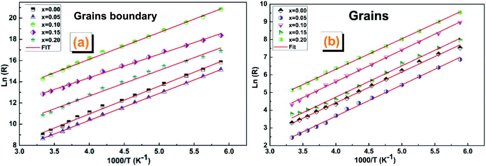 | ||
| Fig. 11 The Arrhenius plots (ln(R) vs. (1000/T)) corresponding to (a) grain boundaries and (b) gains of (La0.8Ca0.2)1−xBixFeO3 (x = 0.00, 0.05, 0.10, 0.15 and 0.20) compounds. | ||
The activation energy values Ea of the two contributions are collated in Table 6. We note that the Ea values of grain boundaries are slightly higher than those of grains, which indicates a higher resistive behaviour than that of grains.
| x | 0.00 | 0.05 | 0.10 | 0.15 | 0.20 |
| Ea of grains (eV) | 0.1500 | 0.1525 | 0.1548 | 0.1521 | 0.1489 |
| Ea of grains boundary (eV) | 0.2267 | 0.2199 | 0.2175 | 0.1978 | 0.2079 |
4.2 Dielectric relaxation study
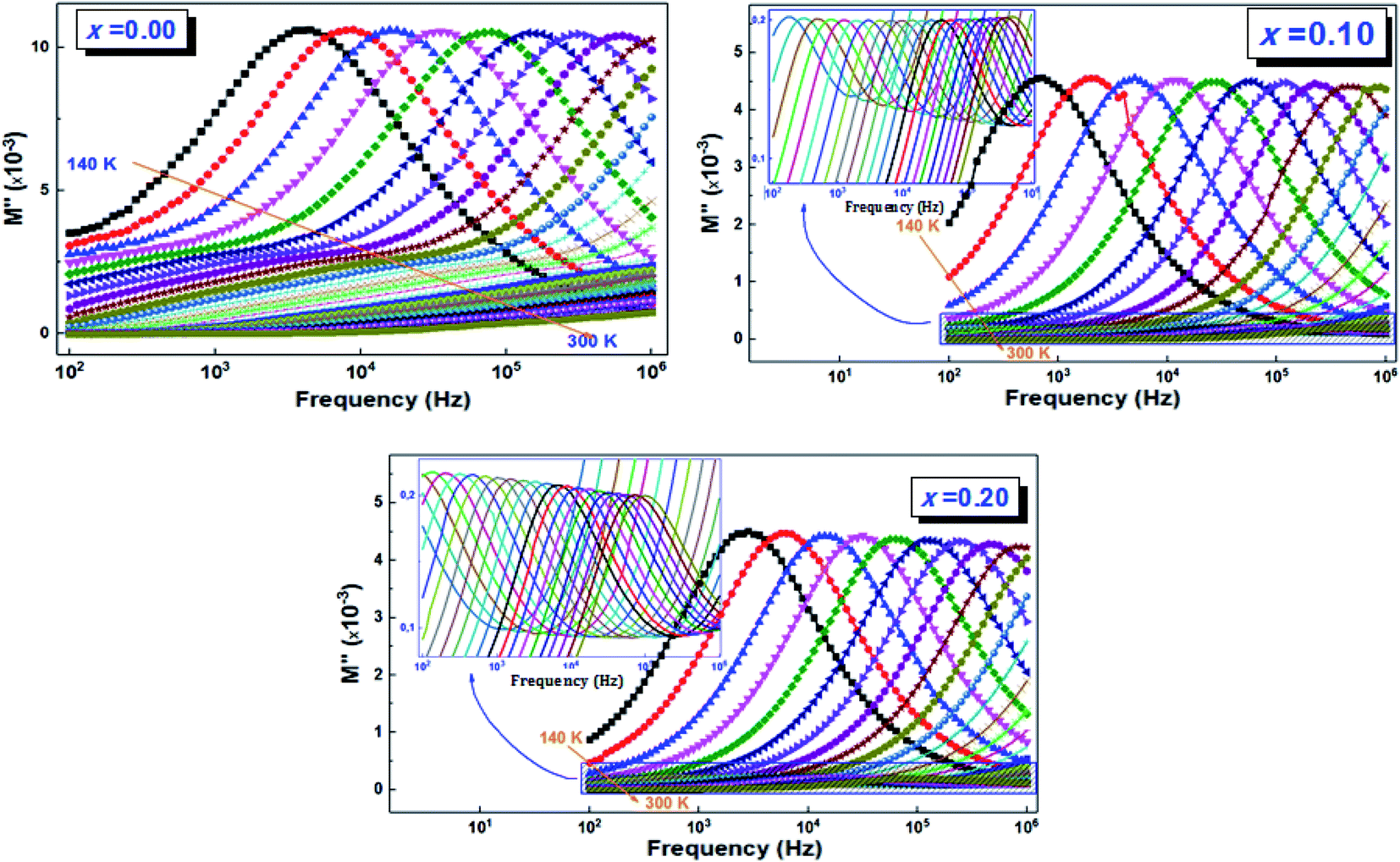 | ||
| Fig. 12 Variation of the imaginary part of the electric modulus (M′′) as a function of frequency and temperature of (La0.8Ca0.2)1−xBixFeO3 (x = 0.00, 0.10, and 0.20) compounds. | ||
For the La0.8Ca0.2FeO3 (x = 0.00) compound, the frequency variation of the imaginary part of the modulus presents a single clear relaxation (peak) in the frequency range f > 5 kHz. This compound shows also very broadening peaks at lower frequencies which their maximums were not detectable. However, the insertion of bismuth into A-site (x ≠ 0.00) induces a change in the trend of the dielectric relaxation process; this peak was clearly registered at lower frequencies and for all temperatures, which is ascribed to the grains contribution. While the second one detected at high frequencies, is attributed to grain boundaries. We also notice that all the peaks move towards the high frequencies when increasing the temperature. This displacement can be linked to the activated thermal energy of the charge carriers in the material, which increases with temperature. In addition, we note that, for a given temperature, the width of the peaks increases with the increase in the bismuth rate and especially for the peaks relating to grain boundary contribution. This may be due to the diffusive movement of the charge carriers and/or the presence of non-uniformities.52
The activation energies (Ea) for both contributions (grains and grain boundaries) were determined using the maximum frequency (fmax) for each temperature and based on the Arrhenius law (eqn (6)):
We present the adjustment results and the activation energy values Ea of the two contributions of all the LCBFO compounds in both Fig. 13(a) and (b).
 | ||
| Fig. 13 Variation of ln(fmax (M′′)) as a function of 1000/T and the activation energies corresponding to (a) gains and (b) at grain boundaries of (La0.8Ca0.2)1−xBixFeO3 (x = 0.00, 0.05, 0.10, 0.15 and 0.20) compounds. | ||
We find that all the determined Ea values are in good agreement with those previously deduced from the study of the imaginary part of the impedance Z′′. Again, and according to the activation energy values, we confirm the polaronic-type relaxation processes in the studied LCBFO compounds.
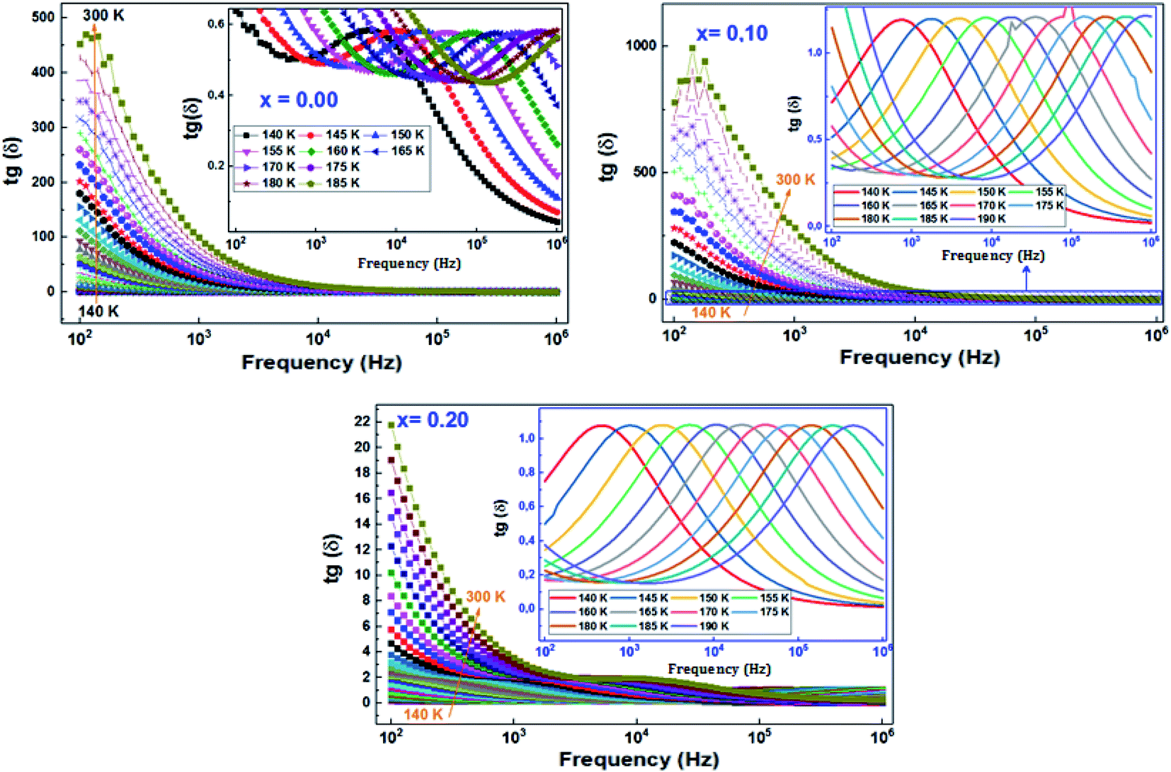 | ||
| Fig. 14 Variation of loss tangent (tanδ) as a function of frequency at different temperatures of (La0.8Ca0.2)1−xBixFeO3 (x = 0.00, 0.10, and 0.20) compounds. | ||
On the other hand, for all compounds, the dielectric tangent loss shows maximum peaks which are found to move towards higher frequency range when increasing temperature, which confirms the thermally activated nature of the relaxation processes.
In order to calculate the activation energies with the Arrhenius relationship, we have determined the maximum frequency corresponding to the relaxation peaks. The tracing of the logarithmic variation of these frequencies as a function of the temperature inverse (Fig. 15) reveals the presence of straight lines whose slopes allowed us to go back to the activation energy (the inset of Fig. 15). It turns out that the variation of this activation energy as a function of the substitution rate is identical to those previously deduced from Z′′ and from modulus M′′, which proves that the relaxations in our compounds are attributed to the same process.
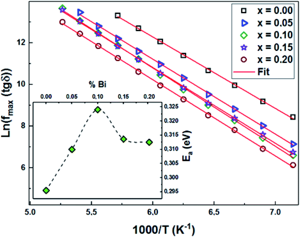 | ||
| Fig. 15 Variation of ln(fmax (tanδ)) as a function of 1000/T and the activation energies corresponding to gains of (La0.8Ca0.2)1−xBixFeO3 (x = 0.00, 0.05, 0.10, 0.15 and 0.20) compounds. | ||
5 Conductivity study
The variation of the product of conductivity and temperature (σac × T) as a function of the inverse of the temperature (1000/T), recorded at different frequencies of all the LCBFO compounds, is shown in Fig. 16. From this figure, we can see that the alternative conductivity is characterized by two different regions suggesting that electrical conduction occurs via two different processes.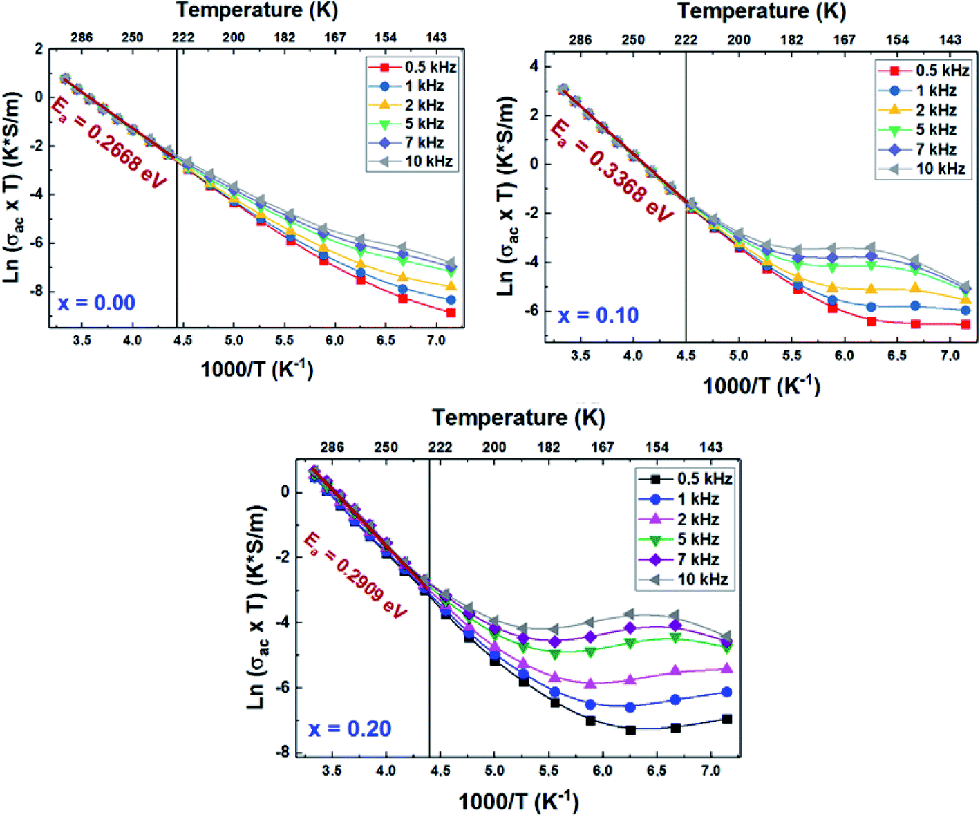 | ||
| Fig. 16 Variation of ln(σac × T) as a function of 1000/T of (La0.8Ca0.2)1−xBixFeO3 (x = 0.00, 0.10 and 0.20) compounds. | ||
In the region of low temperatures (R1: T < 222 K), the conductivity is dependent on both frequency and temperature while for high temperatures (R2: T ≥ 222 K), it only depends on the temperature and shows a linear variation. The conduction process in the first region will be studied in detail in the following, based on the thermal variation of the exponent “s” of Joncher's law. In the second region, we have calculated the activation energies of the alternative conductivity using Arrhenius' law:53
 | (8) |
The calculated activation energy values, from the slopes of each linear adjustment, are shown in Fig. 17. These values are in good agreement with those deduced previously, which suggests that the relaxation process and the electrical conductivity are attributed to the same type of charge carriers, namely the jump of electrons between the states of iron (Fe3+ and Fe4+).
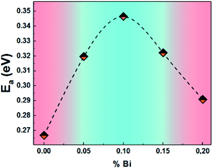 | ||
| Fig. 17 The activation energies of (La0.8Ca0.2)1−xBixFeO3 (x = 0.00, 0.05, 0.10, 0.15 and 0.20) compounds. | ||
The frequency variation of the alternating conductivity for different temperatures of LCBFO compounds is shown in Fig. 18, which shows that the alternating conductivity is almost constant at low frequencies and increases with increasing temperature. This behaviour corresponds to the dc conductivity and confirms the decrease in resistance when the temperature increases. In high frequency regions, the alternating conductivity becomes frequency dependent.
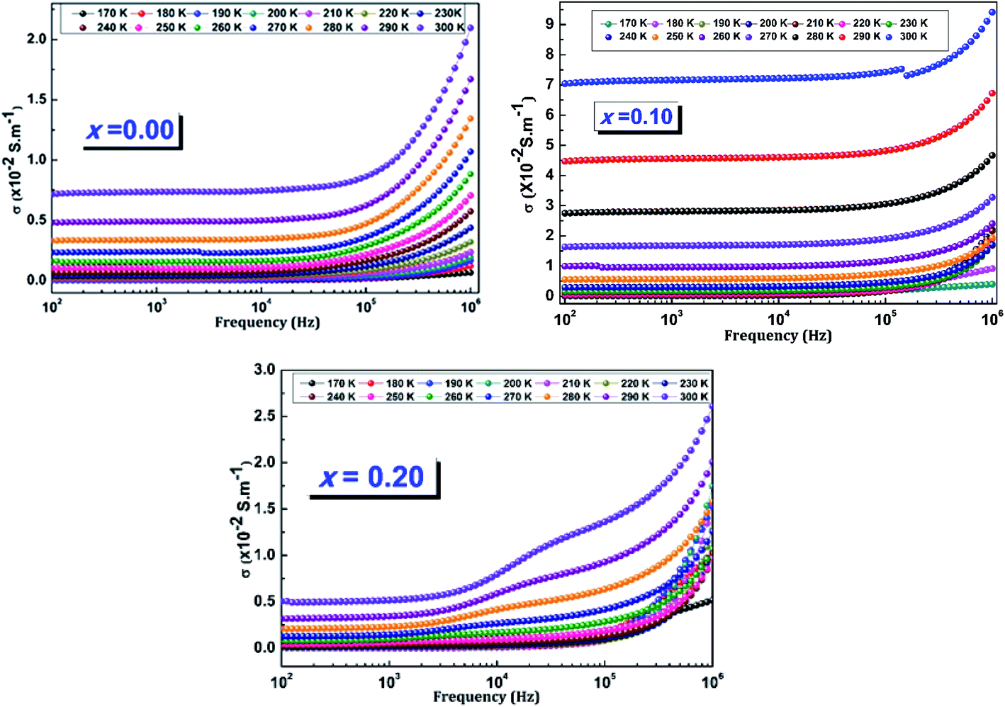 | ||
| Fig. 18 Variation of the ac-conductivity (σac) as a function of frequency at different temperatures of (La0.8Ca0.2)1−xBixFeO3 (x = 0.00, 0.10 and 0.20) compounds. | ||
The ac conductivity curves have been adjusted according to a power law known as Joncher:
| σac(ω,T) = σdc + A × ωs(T) | (9) |
| T (K) | σdc (×10−5 S m−1) | A (×10−7) | S |
|---|---|---|---|
| x = 0.00 | |||
| 140 | 0.45 | 2.34 | 0.23 |
| 150 | 0.63 | 1.78 | 0.31 |
| 160 | 0.02 | 1.96 | 0.36 |
| 170 | 0.05 | 1.24 | 0.47 |
| 180 | 0.12 | 1.75 | 0.57 |
| 190 | 0.4 | 9.46 | 0.63 |
| 200 | 0.72 | 4.38 | 0.72 |
| 210 | 0.11 | 2.698 | 0.82 |
| 220 | 2.04 | 2.99 | 0.91 |
|
|||
| x = 0.10 | |||
| 140 | 5.87 | 2.87 | 0.34 |
| 150 | 7.93 | 5.87 | 0.40 |
| 160 | 4.97 | 1.74 | 0.46 |
| 170 | 3.31 | 2.23 | 0.53 |
| 180 | 50.5 | 3.65 | 0.61 |
| 190 | 87.3 | 4.75 | 0.75 |
| 200 | 136.4 | 1.44 | 0.92 |
| 210 | 202.7 | 1.17 | 0.94 |
| 220 | 287.2 | 6.16 | 1.00 |
|
|||
| x = 0.20 | |||
| 140 | 0.03 | 5.76 | 0.30 |
| 150 | 0.08 | 2.56 | 0.46 |
| 160 | 0.09 | 3.24 | 0.59 |
| 170 | 0.07 | 4.25 | 0.68 |
| 180 | 0.22 | 3.51 | 0.76 |
| 190 | 0.63 | 1.67 | 0.83 |
| 200 | 2.23 | 7.33 | 0.87 |
| 210 | 8.57 | 1.26 | 0.91 |
| 220 | 16.60 | 1.19 | 0.94 |
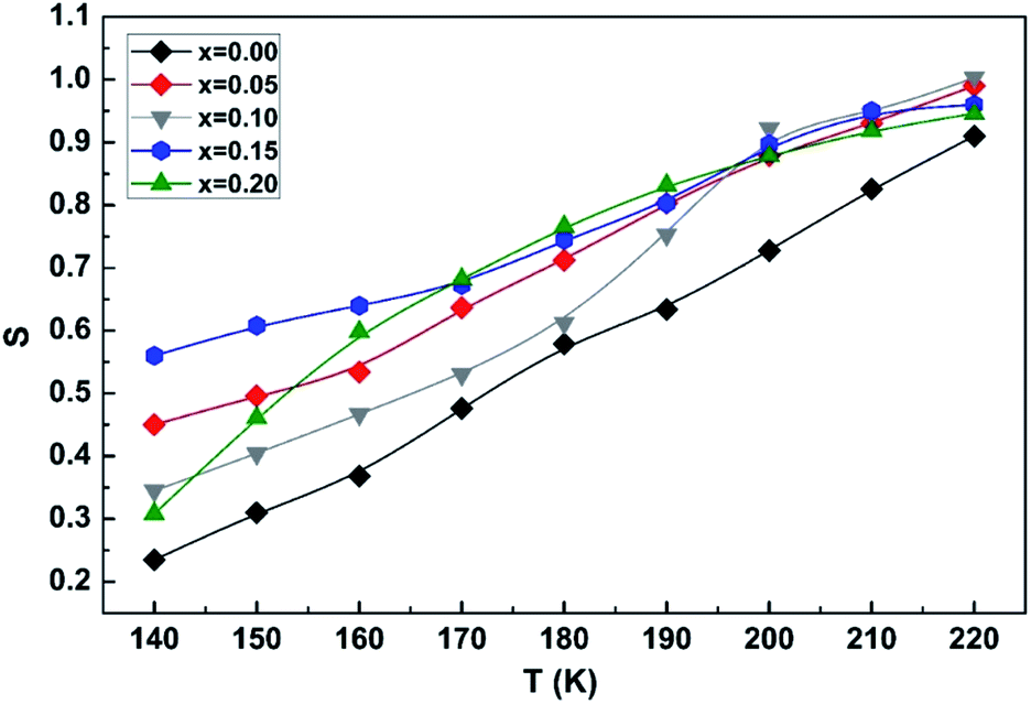
As described before, the “s” parameter of Jonscher's law is of great interest since its thermal variation allows us to identify the conduction process among the four known models.54
The variation of the exponent “s” as a function of the temperature for the LCBFO compounds is shown in Fig. 19.
 | ||
| Fig. 19 Variation of the s exponent as a function of temperature of (La0.8Ca0.2)1−xBixFeO3 (x = 0.00, 0.05, 0.10, 0.15 and 0.20) compounds. | ||
We notice that “s” increases with increasing temperature. Thus, the NSPT model (small polaron tunnel conduction model) seems to be the most suitable to explain the conduction mechanism in the sol–gel compounds studied.
6 Conclusion
The present work has reported the results of the electrical and dielectric studies of (La0.8Ca0.2)1−xBixFeO3 (x = 0.00, 0.05, 0.10, 0.15 and 0.20) (LCBFO) compounds synthesized using a sol–gel method and annealed at T = 800 °C. The electrical properties of our compounds have shown a strong dependence on temperature and frequency. The frequency dispersion of the real and imaginary components of the complex impedance enable to deduct that the insertion of Bi significantly decreases the resistance, complex impedance diagrams have revealed the presence of arcs not centered on the real axis, suggesting that the conduction of these materials follows the Cole–Cole model. The modeling of Nyquist diagrams, at different temperatures, allowed us to go back to the equivalent electrical circuit describing the behaviour of these compounds. The proposed equivalent electrical circuit is the series association of two circuits [(RGB//CPEGB) with (RG//CG)]. The study of the ac conductivity highlighted the existence of a mechanism by jump of the charge carriers between two successive sites, and showed that the insertion of Bi promotes the improvement of conductivity. Likewise, this study showed that the activation energy (Ea) values coincide with those deduced from the analysis of the spectra of the impedance, which allowed us to conclude that the electrical conduction and the phenomenon of relaxation can be attributed to the same type of charge carriers.Conflicts of interest
There are no conflicts to declare.Acknowledgements
This work was supported by national funds from FCT – Fundação para a Ciência e a Tecnologia, I. P., within the project UID/04564/2020. Access to TAIL-UC facility funded under QREN-Mais Centro Project No. ICT_2009_02_012_1890 is gratefully acknowledged.References
- S. Megahed and W. Ebner, J. Power Sources, 1995, 54, 155 CrossRef CAS.
- M. Sugimoto, J. Am. Ceram. Soc., 1999, 82, 269 CrossRef CAS.
- M. Viret, D. Rubi, D. Colson, D. Lebeugle, A. Forget, P. Bonville and G. Dhalenne, Mater. Res. Bull., 2012, 47, 2294 CrossRef CAS.
- J. Suntivich, H. A. Gasteiger, N. Yabuuchi, H. Nakanishi, J. B. Goodenough and S. H. Yang, Nat. Chem., 2011, 3, 546 CrossRef CAS PubMed.
- B. C. Steele and A. Heinzel, Mater. Sustainable Energy, 2011, 224 Search PubMed.
- I. Sosnowska, T. P. Neumaier and E. Steichele, J. Phys. C: Solid State Phys., 1982, 15, 4835 CrossRef CAS.
- K. Huang, H. Y. Lee and J. B. Goodenough, J. Electrochem. Soc., 1999, 145, 3220 CrossRef.
- M. H. Hung, M. V. M. Rao and D. S. Tsai, Mater. Chem. Phys., 2007, 101, 297 CrossRef CAS.
- A. Delmastro, D. Mazza, S. Ronchetti, M. Vallino, R. Spinicci, P. Brovetto and M. Salis, Mater. Sci. Eng., B, 2001, 79, 140 CrossRef.
- N. N. Toan, S. Saukko and V. Lantto, Phys. B, 2003, 327, 279 CrossRef CAS.
- V. Lantto, S. Saukko, N. N. Toan, L. F. Reyes and C. G. Granqvist, J. Electroceram., 2004, 13, 721 CrossRef CAS.
- D. Wang and M. Gong, J. Appl. Phys., 2011, 109, 114 Search PubMed.
- S. Phokha, S. Pinitsoontorn, S. Rijirawat and S. Maensiri, J. Nanosci. Nanotechnol., 2015, 15, 9171 CrossRef CAS PubMed.
- V. V. Kharton, A. P. Viskup, E. N. Naumovich and V. N. Tikhonovich, Mater. Res. Bull., 1999, 34, 1311 CrossRef CAS.
- J. E. ten Elshof, M. H. R. Lankhorst and H. J. M. Bouwmeester, J. Electrochem. Soc., 1997, 144, 1060 CrossRef.
- S. Komornicki, L. Fournes, J. Grenier, F. Menil, M. Pouchard and P. Hagenmuller, Mater. Res. Bull., 1981, 16, 967 CrossRef CAS.
- M. Vallet-Regí, J. González-Calbet, M. A. Alario-Franco, J.-C. Grenier and P. Hagenmuller, J. Solid State Chem., 1984, 55, 251–261 CrossRef.
- E. K. Abdel-Khalek and H. M. Mohamed, Hyperfine Interact., 2013, 222(1), 57 CrossRef CAS.
- P. Ciambelli, S. Cimino, L. Lisi, M. Faticanti, G. Minelli, I. Pettiti and P. Porta, Appl. Catal., B, 2001, 33, 193 CrossRef CAS.
- L. B. Kong and Y. S. Sheng, Sens. Actuators, B, 1996, 30, 217 CrossRef CAS.
- A. Benali, M. Bejar, E. Dhahri, M. Sajieddine, M. P. F. Graça and M. A. Valente, Mater. Chem. Phys., 2015, 149, 467 CrossRef.
- H. Saoudi, A. Benali, M. Bejar and E. Dhahri, J. Alloys Compd., 2017, 731, 655–661 CrossRef.
- G. Pecchi, M. G. Jiliberto, A. Buljan and E. J. Delgado, Solid State Ionics, 2011, 187, 27 CrossRef CAS.
- S. Smiy, H. Saoudi, A. Benali, M. Bejar and E. Dhahri, Chem. Phys. Lett., 2019, 735, 136765 CrossRef CAS.
- A. Benali, M. Bejar, E. Dhahri, M. F. P. Graça and L. C. Costa, J. Alloys Compd., 2015, 653, 506 CrossRef CAS.
- A. Benali, A. Souissi, M. Bejar, E. Dhahri, M. F. P. Graca and M. A. Valente, Chem. Phys. Lett., 2015, 637, 7 CrossRef CAS.
- H. Issaoui, A. Benali, M. Bejar, E. Dhahri, M. P. F. Graca, M. A. Valente and B. F. O. Costa, Chem. Phys. Lett., 2019, 731, 136588 CrossRef CAS.
- H. Issaoui, A. Benali, M. Bejar, E. Dhahri and B. F. O. Costa, Hyperfine Interact., 2020, 241, 26 CrossRef CAS.
- H. Issaoui, A. Benali, M. Bejar, E. Dhahri, R. F. Santos, N. Kus, B. A. Nogueira, R. Fausto and B. F. O. Costa, J. Supercond. Novel Magn., 2018, 32(6), 1571–1582 CrossRef.
- R. Hamdi, A. Tozri, E. Dhahri and L. Bessais, Intermetallics, 2017, 89, 118–122 CrossRef CAS.
- R. A. Young, The Rietveld Method, Oxford University Press, New York, 1993 Search PubMed.
- V. Goldschmidt, Geochemistry, Oxford University Press, 1958 Search PubMed.
- Y. Tokura and Y. Tomioka, J. Magn. Magn. Mater., 1999, 200, 1 CrossRef CAS.
- A. Guinier, in Théorie et Technique de la radiocristallographie, ed. X. Dunod, 3rd edn, 1964, p. 462 Search PubMed.
- P. Goel and K. L. Yadav, J. Mater. Sci., 2007, 42(11), 3928 CrossRef CAS.
- F. Bordi, C. Cametti and R. H. Colby, J. Phys.: Condens. Matter, 2004, 16, 1423 CrossRef.
- N. Rezlescu, P. D. Popa, E. Rezlescu and C. Doroftei, J. Phys., 2008, 53, 545 CAS.
- Q. Rong, Y. Zhang, T. Lv, K. Shen, B. Zi, Z. Zhu and Q. Liu, Nanotechnology, 2018, 29(14), 145503 CrossRef PubMed.
- A. Bougoffa, J. Massoudi, M. Smari, E. Dhahri and K. Khirouni, J. Mater. Sci.: Mater. Electron., 2019, 30(24), 21031 CrossRef.
- B. Bechera, P. Nayak and R. N. P. Choudhary, Mater. Res. Bull., 2008, 43, 401 CrossRef.
- M. Haibado, B. Louati, F. Hlel and K. Guidara, J. Alloys Compd., 2011, 509, 6083 CrossRef.
- D. Bouokkeze, J. Massoudi, W. Hzez, M. Smari, A. Bougoffa and K. Khirouni, RSC Adv., 2019, 9(70), 40940 RSC.
- A. Kumar, B. P. Singh, R. N. P. Choudhary and A. K. Thakur, Mater. Chem. Phys., 2006, 99, 150 CrossRef CAS.
- K. K. Srivastava, A. Kumar, O. S. Panwar and L. N. Lakshminarayan, J. Non-Cryst. Solids, 1979, 3, 33 Search PubMed.
- M. Shivanand, B. Ponraj, R. Bhimireddi and K. B. R. Varma, J. Am. Ceram. Soc., 2017, 100, 2641 CrossRef.
- V. G. Nair, A. Das, V. Subramanian and P. N. Santhosh, J. Appl. Phys., 2013, 113, 213907 CrossRef.
- R. Ertugrul and A. Tataroglu, Chem. Phys. Lett., 2012, 29, 077304 Search PubMed.
- P. B. Macedo, C. T. Moynihan and R. Bose, Phys. Chem. Glasses, 1972, 13(6), 171 CAS.
- A. Shukla, R. N. P. Choudhary and A. K. Thakur, J. Phys. Chem. Solids, 2009, 70(11), 1401 CrossRef CAS.
- A. Kumar, P. Kumari, A. Das, G. D. Dwivedi, P. Shahi, K. K. Shukla, A. K. Ghosh, A. K. Nigam, K. K. Chattopadhyay and S. Chatterjee, J. Solid State Chem., 2013, 208, 120 CrossRef CAS.
- S. Hcini, A. Selmi, H. Rahmouni, A. Omri and M. L. Bouazizi, Ceram. Int., 2017, 43(2), 2529 CrossRef CAS.
- C. T. Moynihan, Solid State Ionics, 1998, 105, 175 CrossRef CAS.
- M. Ganguli, M. Harish Bhat and K. J. Rao, Phys. Chem. Glasses, 1999, 40(6), 297 CAS.
- R. L. Frost, P. A. Williams, J. T. Kloprogge and P. Leverett, Raman Spectrosc., 2011, 32, 906 CrossRef.
| This journal is © The Royal Society of Chemistry 2020 |