
 Open Access Article
 This Open Access Article is licensed under a Creative Commons Attribution-Non Commercial 3.0 Unported Licence
Coupling of digital image processing and three-way calibration to assist a paper-based sensor for determination of nitrite in food samples†
Zohreh Almasvandia,
Ali Vahidinia a,
Ali Heshmatia,
Mohammad Mahdi Zangenehbc,
Hector C. Goicoechead and
Ali R. Jalalvand*e
a,
Ali Heshmatia,
Mohammad Mahdi Zangenehbc,
Hector C. Goicoechead and
Ali R. Jalalvand*e
aDepartment of Nutrition and Food Hygiene, School of Medicine, Hamadan University of Medical Sciences, Hamadan, Iran
bDepartment of Clinical Sciences, Faculty of Veterinary Medicine, Razi University, Kermanshah, Iran
cBiotechnology and Medicinal Plants Research Center, Ilam University of Medical Sciences, Ilam, Iran
dLaboratorio de Desarrollo Analítico y Quimiometría (LADAQ), Catedra de Química Analítica I, Universidad Nacional del Litoral, Ciudad Universitaria, CC242 (S3000ZAA), Santa Fe, Argentina
eResearch Center of Oils and Fats, Kermanshah University of Medical Sciences, Kermanshah, Iran. E-mail: ali.jalalvand1984@gmail.com
First published on 8th April 2020
Abstract
In this work, a novel and very interesting analytical methodology based on coupling of digital image processing and three-way calibration has been developed for determination of nitrite in food samples. Nitrite in contact with Griess reagent is able to produce a red-colored azo dye whose color intensity is correlated with nitrite concentration and here, a piece of Whatman filter paper impregnated with Griess reagent was used as the platform of the sensor and a SONY Xperia Z5 cell phone was used for image capturing from the sensor surface. To generate second-order data, the F-number of the camera's sensor was changed as an instrumental parameter. Two calibration models were constructed by unfolded partial least squares-residual bilinearization (U-PLS/RBL) and multiway-PLS/RBL (N-PLS/RBL) and then, their performance for prediction of nitrite concentration in test samples was evaluated and the results confirmed a good performance for U-PLS/RBL (REP = 3.25 ppm, RMSEP = 8.82 ppm, RMSEC = 4.62 ppm, Q2 = 0.99, γ−1 = 0.05 and LOD = 0.1 ppm) which was better than that for N-PLS/RBL (REP = 13.98 ppm, RMSEP = 37.86 ppm, RMSEC = 6.46 ppm, Q2 = 0.98, γ−1 = 0.07 and LOD = 0.15 ppm) in predicting concentration of nitrite in test samples which motivated us to choose it for the analysis of cabbage, carrot, lettuce, watermelon, onion, potato, kielbasa and sausage as real samples.
Introduction
Nitrite which is used as a fertilizer in agriculture and as a preservative of foods in food industries plays a key role in hypoxic nitric oxide homeostasis and blood flow regulation.1 Uncontrolled levels of nitrite (middle: 50 to <100 mg g−1 fresh weight of food, high: 100 to <250 mg g−1 fresh weight of food and very high: >250 mg g−1 fresh weight of food) in foods is dangerous for public health because of its interaction with dietary components in the stomach producing carcinogenic nitrosamines.2,3 The presence of nitrite in the blood stream can disturb oxygen transport in the blood because of its ability to convert oxyhemoglobin into methemoglobin.4 Therefore, monitoring of nitrite in foods is very important and several techniques based on organic chromophores,5–7 electrochemical detection,8 and ion chromatography,9,10 have been reported for determination of nitrite. Many of these approaches need sophisticated instruments and are time consuming. Therefore, developing novel methods for the determination of nitrite which are rapid and low-cost is highly needed.Paper-based sensors (PBSs) are very interesting, because they are able to simple, low-cost, sensitive and selective determination of the analyte.11–16 Furthermore, their determination procedure is simple which needs small volumes of sample and a simple equipment. Therefore, a PBS is a good choice to develop a novel analytical method for rapid and sensitive determination of nitrite. Griess reagent (3-nitroaniline, 1-naphthylamine and hydrochloric acid) is able to selective reaction with nitrite to produce a red-colored azo dye whose color intensity is correlated with nitrite concentration. Therefore, a PBS impregnated with Griess reagent is able to produce a red color in the presence of nitrite. After image capturing from the PBS surface, the image can be digitally processed by MATLAB to extract the intensities of the red pixels.
Chemometrics is chemical discipline which uses mathematical and statistical methods to extract useful information from chemical data.17 There are many reports on applications of chemometric methods for processing of chemical data for different purposes.18–22 According to the IUPAC recommendation, analytical calibration relates instrumental signals to analyte concentrations. Chemometrics enables us to better calibration model building and among the existing approaches, multi-way calibration is very interesting. Multi-way calibration is based on many instrumental signals per sample which can be meaningfully organized into a certain mathematical object with more modes than a vector, for example, as a matrix or an array.17 The most important advantage of multi-way calibration is determination of the analyte(s) of interest in the presence of uncalibrated interference which is known as second-order advantage. Multi-way calibration also increases the sensitivity of the analytical method due to the measurement of redundant data which decreases the relative impact of the noise in the data and selectivity is also increased because each new instrumental mode contributes positively to the overall selectivity.23,24 Three-way calibration needs second-order data which can be generated by changing one instrumental parameter. The F-number (F) of the camera's sensor which controls the size of the circular opening (entrance pupil) allows light to reach camera's sensor.25 The F can be used as an instrumental parameter to generate second-order data for building three-way calibration models. In this work, two second-order algorithms including unfolded partial least squares-residual bilinearization (U-PLS/RBL) and multiway-PLS/RBL (N-PLS/RBL) are used and in the N-PLS/RBL and U-PLS/RBL methodologies, the first step consists of establishing a relationship between the measured calibration signals and the known calibration concentrations, without considering the test sample data. Once this is done, a post calibration RBL procedure applied to the test sample signals is introduced, allowing one to model the presence of unexpected components and to accurately estimate the analyte concentration.
In the present study, we have developed a novel analytical methodology for rapid and sensitive determination of nitrite in food samples. To achieve this goal, rectangular pieces of the Whatman filter paper were cut which acted as the platform of the PBSs. Then, the PBSs were impregnated with Griess reagent which were able to produce a red color in contact with nitrite. By a SONY Xperia Z5 cell-phone, eight images under different F values ranging in 1–8 were taken from the surface of each PBS and then, the images were transferred to the MATLAB environment and by the existing commands, the intensities of the red color of each image were extracted as a vector. Therefore, for each PBS, eight vectors were extracted which arranged into a matrix and matrices related to a set of samples were arranged into a three-way data array. The U-PLS/RBL and N-PLS/RBL were used as second-order algorithms for building three-way calibration models using the data obtained from the calibration set. Then, a test set was designed to examine the performance of U-PLS/RBL and N-PLS/RBL in predicting concentration of nitrite in synthetic samples. Finally, the best model was used to the analysis of real samples towards nitrite concentration. The schematic representation of the steps of our study is shown in Scheme 1.
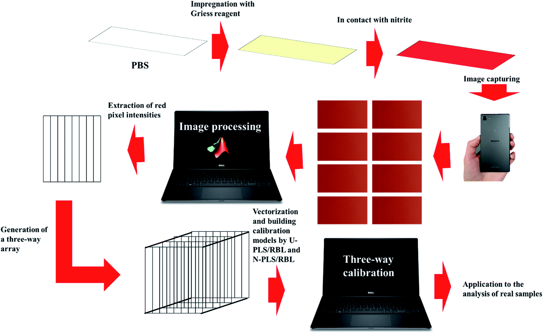 | ||
| Scheme 1 Schematic representation of the procedure developed in this work for the sensing of nitrite. | ||
Experimental and theoretical details
Chemicals and solutions
Sodium nitrite, HCl, 3-nitroaniline, 1-naphthylamine, acetone, ethanol, Whatman filter paper and the other reagents used in this study were purchased from Sigma. All the chemicals were of analytical grade and used as received without any further purifications. Doubly distilled water (DDW) was used to prepare all the solutions. Stock solution of nitrite with a concentration of 1000 ppm was prepared in deionized water and working solutions of nitrite were prepared by applying suitable dilutions to its stock solution. A DDW/ethanol mixture (50![[thin space (1/6-em)]](https://www.rsc.org/images/entities/char_2009.gif) :50, v/v%) was used to prepare Griess reagent. 3-Nitroaniline (2 × 10⁻³ M), 1-naphthylamine (5 × 10⁻³ M) and hydrochloric acid (1 × 10⁻³ M) were added to DDW/ethanol mixture (50:50, v/v%) to prepare the Griess reagent.
:50, v/v%) was used to prepare Griess reagent. 3-Nitroaniline (2 × 10⁻³ M), 1-naphthylamine (5 × 10⁻³ M) and hydrochloric acid (1 × 10⁻³ M) were added to DDW/ethanol mixture (50:50, v/v%) to prepare the Griess reagent.
Instruments and software
A SONY Xperia Z5 cell-phone with a 24 MP camera was used for capturing the images. A wooden box was designed for the cell-phone which had a sample holder located under the camera lens for putting the sensor in it which helped us to had a better image capturing process. The cell-phone was located on the wooden box and the sample holder was located under the camera of the cell-phone. The sample holder had six small LED lamps which were located around its inner side. With the help of sample holder, we could put the sensor under the camera of the cell-phone with a distance of 1 cm from the camera lens. The wooden box helped us to had a repeatable position for landing the sensors under the camera and also helped us to had a same illumination condition for all the sensors. Therefore, we had a same condition for image capturing from the surface of the all sensors. Image processing was performed in MATLAB environment (Version 7.5) using the commands provided by its image processing toolbox. All the calculations related to U-PLS/RBL and N-PLS/RBL and elliptical joint confidence region (EJCR) were performed in MATLAB. The routines of U-PLS/RBL and N-PLS/RBL were obtained from their owners without any modifications. All the calculations were performed on a Dell XPS laptop operating under a Windows 10 (professional version).Operating procedure
Rectangular pieces (1.5 cm × 3 cm) of Whatman filter paper were cut which were used as the platform of the sensor. The papers were immersed into the Griess reagent and dried at room temperature (25 °C). The sensors were immersed into different nitrite solutions having different concentrations of nitrite and after drying them at room temperature by keeping them for 15 min, were transferred to the sample holder. Then, eight images were taken from the surface of each sensor by using eight different F values for camera's lens ranging in 1–8. Afterwards, the images were transferred into MATLAB environment and the RGB matrix (red (R), green (G) and blue (B)) of each image was extracted and then, the intensity of the red pixels were separated to produce a vector for each image. For each sensor, eight images were taken which produced eight vectors and by arranging them into a matrix, we could obtain a data matrix for each sensor. To remove any background variation from sensor-to-sensor, a sensor was immersed into the Griess reagent and without contacting it with nitrite (blank sensor), eight images were taken from its surface. Then, its data matrix was subtracted from the data matrices related to the other sensors in contact with nitrite. We called this procedure as “background elimination procedure”. To build calibration models by U-PLS/RBL and N-PLS/RBL, a calibration set having sixteen samples with different nitrite concentrations was designed and the data matrices related to its samples were arranged into a three-way data array (second-order data). The performance of the developed calibration models by U-PLS/RBL and N-PLS/RBL was examined by verifying their ability for prediction of nitrite concentration in test samples having random nitrite concentrations. Finally, the best algorithm was chosen for determination of nitrite in real samples. To evaluate the performance of the developed methodology in this work, we compared its results for the analysis of real samples with HPLC (KNAUER) equipped with an ODS column (length 250 mm, internal diameter 4.6 mm and particle diameter 5 μm) and a UV detector (λmax = 207 nm) as reference method. The mobile phase was consisted of acetonitrile:H2O (55/45 v/v).
Preparation of real samples
To extract nitrite from cabbage, carrot, lettuce, watermelon, onion, potato, kielbasa (four commercial brands including Andre, Sham Sham, Armen and Dalahoo) and sausage (four commercial brands including Andre, Sham Sham, Armen and Solico) samples, exact amounts of crushed samples (115.915 g cabbage, 156.48 g carrot, 58.7 g lettuce, 197.4 g watermelon, 131.200 g onion, 100.07 g potato, kielbasa (120.9 g Andre, 83.45 g Sham Sham, 90.13 g Armen and 169.8 g Dalahoo) and sausage (49.78 g Andre, 60.48 g Sham Sham, 133 g Armen and 53.15 g Solico)) were left in DDW at 70 °C under stirring for 15 min and then, the remained liquids were filtered.26 For each real sample, 100 μL of its extract was dropped onto the PBS surface and left to be dried at room temperature. Then, eight images upon applying different F values were captured from each PBS surface which were digitally processed and converted to a matrix. The real samples were further spiked with different concentrations of nitrite and used for further investigation of the performance of the developed methodology.Summarized theoretical details
| yu = tuTv | (1) |
| tu = (WTP)−1WTvec(Xu) | (2) |
By the presence of uncalibrated interferents in the test samples, the sample scores described by eqn (2) are not suitable for predicting concentration of the analyte. In this case, the residuals are larger than the typical instrumental noise assessed by replicate measurements which can be handled by RBL. The required information about mathematical aspects of RBL can be found in ref. 30, 32 and 33.
The N-PLS employs concentration information in the calibration step without including data for the unknown sample. The N-PLS uses the calibration data array and the vector of the calibration concentrations to obtain sets of loadings as well as regression coefficients. The number of latent variables is determined by the LOOCV. In the absence of uncalibrated interferents in the test sample, the regression coefficients are used to predict concentration of the analyte otherwise, the residuals will be abnormally large in comparison with the typical instrumental noise level and the scores would not be suitable for prediction of the analyte concentration and this situation can be handled by RBL.
 | (3) |
 | (4) |
 | (5) |
 | (6) |
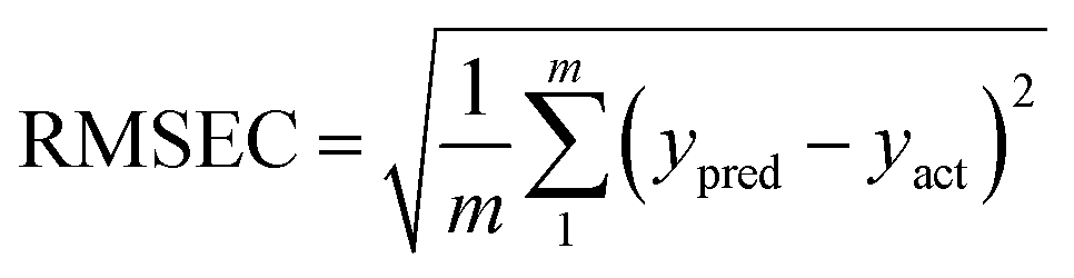
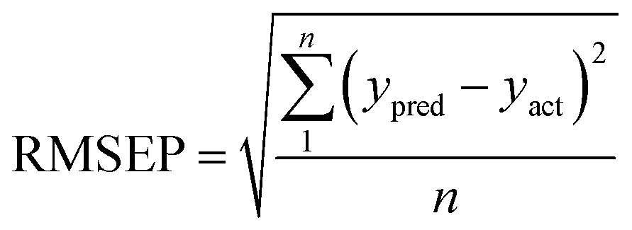
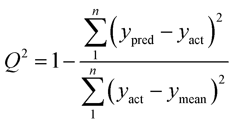
Some analytical figures of merit (AFOM) such as inverse of the analytical sensitivity (γ), γ−1 = sx/SENn where sx is the instrumental noise and SENn is the sensitivity,34 sx and SENn are averages of the values corresponding to 10 test samples and the limit of detection, LOD = 3.3γ−1,35 were also calculated.
The EJCR was used to compare the accuracy and precision of U-PLS/RBL and N-PLS/RBL in predicting concentration of nitrite in test samples. The EJCR works based on ordinary least squares (OLS) analysis of predicted concentrations versus nominal concentrations to calculate intercept and slope which are compared with their theoretically expected values (intercept = 0 and slope = 1, ideal point).36 If the ellipses contain the ideal point, there isn't any significant difference at the level of 95% confidence and the size of the ellipses is correlated with precision of the method, smaller size corresponds to higher precision.37
Results and discussion
Building calibration models
In order to develop calibration models, a set of sixteen samples having different concentrations of nitrite ranging in 0.5–1000 ppm (Table 1) was prepared and their images were captured which can be seen in Fig. 1. As stated in previous sections, for each sample, eight images upon applying different F values to the camera's lens were taken. After transferring the images to the MATLAB environment, each image produced an array (2160 × 3840 × 3) in MATLAB workspace which was used for digital image processing. A home-made m-file was used for processing the images which facilitated performing digital image processing. Background subtraction was performed as a useful pre-processing technique which helped us to remove variations existed from sample-to-sample. To achieve this goal, eight images were taken from the surface of a PBS impregnated with Griess reagent without contacting with nitrite which we called it as “blank sample” and then, the images were transferred to MATLAB environment and a data matrix was constructed by the vectors obtained from their red pixel intensities. This data matrix was subtracted from the data matrix obtained from the PBSs in contact with nitrite. After processing the eight images captured from the surface of each sensor, the intensities of their red pixels were extracted to obtain eight vectors (8 × 3840). Therefore, each sensor produced a matrix and then, the data matrices obtained for the calibration set were joint to build a three-way data array. The second-order data obtained by the procedure mentioned above was used for building calibration models by N-PLS/RBL and U-PLS/RBL.| Nominal concentrations (ppm) | Predicted concentrations (ppm) of the test set | ||
|---|---|---|---|
| Calibration set | Test set | U-PLS/RBL | N-PLS/RBL |
| 0.5 | 1.0 | 1.01 | 0.90 |
| 1.0 | 2.5 | 2.48 | 2.65 |
| 2.5 | 15.0 | 15.11 | 16.34 |
| 5.0 | 50.0 | 49.21 | 45.14 |
| 7.5 | 90.0 | 91.32 | 81.12 |
| 10.0 | 150.0 | 147.29 | 169.22 |
| 20.0 | 300.0 | 306.66 | 324.50 |
| 40.0 | 500.0 | 488.35 | 561.01 |
| 60.0 | 700.0 | 721.57 | 761.33 |
| 80.0 | 900.0 | 911.12 | 975.98 |
| 100.0 | — | — | — |
| 200.0 | — | — | — |
| 400.0 | — | — | — |
| 600.0 | — | — | — |
| 800.0 | — | — | — |
| 1000.0 | — | — | — |
| RMSEP (ppm) | — | 8.82 | 37.86 |
| REP (ppm) | — | 3.25 | 13.98 |
| RMSEC (ppm) | — | 4.62 | 646 |
| Q2 | — | 0.99 | 0.98 |
| γ−1 | — | 0.05 | 0.07 |
| LOD (ppm) | — | 0.1 | 0.15 |
 | ||
| Fig. 1 The images recorded for the samples of the calibration set: (a) 0.5, (b) 1.0, (c) 2.5, (d) 5.0, (e) 7.5, (f) 10, (g) 20, (h) 40, (i) 60, (j) 80, (k) 100, (l) 200, (m) 400, (n) 600, (o) 800 and (p) 1000 ppm nitrite. | ||
Determination of the number of latent variables is critical to build a calibration model and because of that we have used LOOCV to determine the number of latent variables for building calibration models by N-PLS/RBL and U-PLS/RBL. The LOOCV allowed us to determine two and one latent variables for N-PLS/RBL and U-PLS/RBL, respectively. Then, the calibration models according to the detected latent variables were used for next sections.
Validation of the developed calibration models
In order to verify the performance of the calibration models developed by N-PLS/RBL and U-PLS/RBL for predicting nitrite concentration in synthetic samples, a test set containing ten samples with different concentrations of nitrite ranging in 1–900 ppm was designed (Table 1) and by the same data acquisition procedure used for the calibration set, the data of the test set were recorded. The images which were recorded for the test set are shown in Fig. 2. The images were then transferred to MATLAB environment and after extraction of the red pixel intensities, their data were used to build three-way calibration models. The U-PLS/RBL and N-PLS/RBL were run on the test set data to predict concentration of nitrite in test samples and the results are shown in Table 1. | ||
| Fig. 2 The images recorded for the samples of the test set: (a) 1, (b) 2.5, (c) 15, (d) 50, (e) 90, (f) 150, (g) 300, (h) 500, (i) 700 and (j) 900 ppm nitrite. | ||
The next attempt will be focused on comparing the performance of U-PLS/RBL and N-PLS/RBL in predicting concentration of nitrite in test set samples which will be expanded with more details in next section.
In order to compare the performance of U-PLS/RBL and N-PLS/RBL in predicting concentration of nitrite and choosing the best algorithm for the analysis of real samples, statistical parameters described in Model efficacy estimation section were determined for the test set. The EJCR performed an ordinary lest squares for the regression of the actual (nominal) concentrations of nitrite in the test set versus predicted concentrations by U-PLS/RBL and N-PLS/RBL. The outputs of the EJCR were ellipses and as stated in Model efficacy estimation section, if the ellipses include the ideal point the predicted and nominal values are not significantly different. The size of ellipses is correlated with the precision of the method, smaller sizes confirm higher precisions.37 The results related to the calculation of REP, RMSEP, RMSEC, Q2, γ−1 and LOD are collected in Table 1. As can be seen, the U-PLS/RBL was more successful than N-PLS/RBL in predicting concentration of nitrite in test samples. The results of EJCR are shown in Fig. 3 and as can be seen, an ellipse with a smaller size which involves the ideal point was obtained for U-PLS/RBL while the ellipse of N-PLS/RBL was bigger than that of U-PLS/RBL which didn't contain the ideal point.
 | ||
| Fig. 3 Ellipses obtained by the EJCR method for the analysis of test samples by N-PLS/RBL (blue ellipse) and U-PLS/RBL (red ellipse). The black point shows the ideal point. | ||
According to the results mentioned above, the U-PLS/RBL was preferred for the analysis of real samples towards determination of nitrite.
Application of the developed method to the analysis of real samples
After preparation of real samples, the U-PLS/RBL was used to the prediction of nitrite concentration in real samples. After preparation of the extracts of the real samples, the PBSs impregnated with Griess reagent were immersed in the extract and then, eight images were recorded from their surface. The images captured from the surface of the PBSs are shown in Fig. S1 (ESI†). By the same procedure used for data processing for analysing of synthetic samples, the real samples were analyzed. The results of the analysis of different real samples have been collected in Table 2. In order to further verification of the capability of the developed method for determination of nitrite in real matrices, the samples were spiked with different concentrations of nitrite and then, the recoveries were calculated which can be seen in Table 2. As can be seen, good recoveries were obtained which confirmed the capability of the method for the analysis of real samples.| Samples | Non-spiked samples | Spiked samples | ||||||||||||
|---|---|---|---|---|---|---|---|---|---|---|---|---|---|---|
| U-PLS/RBL | Reference method | U-PLS/RBL | Reference method | |||||||||||
| Added | Found (% rec.c) | Added | Found (% rec.) | Added | Found (% rec.) | Added | Found (% rec.) | Added | Found (% rec.) | Added | Found (% rec.) | |||
| a All the concentrations are in ppm.b Not detected.c Recovery. | ||||||||||||||
| Cabbage | 0.2 | 0.18 | 500 | 521.11 (104) | 250 | 243.5 (97.4) | 50 | 50.4 (100.8) | 500 | 505.1 (101) | 250 | 248.4 (99.4) | 50 | 50 (100) |
| Carrot | N.D.b | N.D. | 500 | 510 (101.9) | 200 | 189 (94.5) | 50 | 51 (101.9) | 500 | 502 (100.4) | 200 | 195 (97.5) | 50 | 50 (100) |
| Lettuce | 0.18 | 0.17 | 450 | 445.5 (99) | 300 | 308.1 (102.6) | 50 | 49.2 (98.4) | 450 | 452.4 (100.5) | 300 | 303.9 (101.3) | 50 | 49.6 (99.2) |
| Watermelon | N.D. | N.D. | 500 | 515.7 (103.1) | 200 | 188.6 (94.3) | 100 | 102 (102) | 500 | 496.6 (99.3) | 200 | 197 (98.5) | 100 | 96 (96) |
| Onion | 25 | 26.3 | 400 | 411.5 (102.8) | 250 | 255.9 (102.3) | 20 | 19.7 (98.5) | 400 | 411.5 (102.8) | 250 | 254.3 (101.7) | 20 | 20.5 (102.4) |
| Potato | 0.71 | 0.77 | 500 | 510 (102) | 100 | 106.6 (106.2) | 10 | 9.7 (97) | 500 | 488 (97.6) | 100 | 107.5 (107) | 10 | 10.1 (101) |
| Kielbasa (Andre) | 0.21 | 0.20 | 100 | 104.9 (104.7) | 10 | 9.9 (99) | — | — | 100 | 94 (94) | 10 | 10.2 (102) | — | — |
| Kielbasa (Armen) | 0.28 | 0.26 | 500 | 511.1 (102.2) | 50 | 49.5 (99) | — | — | 500 | 491 (98.2) | 50 | 50.3 (100.6) | — | — |
| Kielbasa (Sham Sham) | 12.5 | 12.3 | 500 | 493.6 (98.7) | 50 | 50.9 (101.8) | — | — | 500 | 491.1 (98.2) | 50 | 49.6 (99.2) | — | — |
| Kielbasa (Dalahoo) | 0.31 | 0.30 | 700 | 731.3 (104.3) | 500 | 481.2 (96.2) | — | — | 700 | 731.3 (104.2) | 500 | 504.3 (100.8) | — | — |
| Sausage (Andre) | 0.23 | 0.25 | 500 | 488.1 (97.6) | 100 | 106.3 (105.9) | — | — | 500 | 492.6 (98.5) | 100 | 97.7 (97.7) | — | — |
| Sausage (Armen) | N.D. | 0.09 | 100 | 96.5 (96.5) | 10 | 10.1 (101) | — | — | 100 | 93.1 (93.1) | 10 | 10.1 (101) | — | — |
| Sausage (Sham Sham) | 14.3 | 15.1 | 200 | 205.5 (102.7) | 100 | 93.2 (93.2) | — | — | 200 | 210.7 (105.1) | 100 | 106.6 (106.6) | — | — |
| Sausage (Silico) | 11.2 |
11.5 |
200 | 208 (103.8) | 20 | 19.7 (98.5) | — | — | 200 | 209.9 (104.7) | 20 | 20.2 (101) | — | — |
Validation of the performance of the developed method in the analysis of real samples
After developing a novel analytical method, as a final step of the study, the performance of the developed method must be compared with a reference method which is very critical to suggest it as a reliable technique for next uses by the other users. Therefore, to achieve this goal, we have used the HPLC as a reference method for the analysis of real samples as well. The results of the HPLC have been collected in Table 2. As can be seen, the results are very near to the ones obtained by the developed method in this study. However, HPLC was acted slightly better than the method developed in this study, but by taking into account that the HPLC is very expensive which needs a time-consuming sample preparation step, we can suggest our method as a reliable, fast (about 25 min is required for the analysis of a real sample) and inexpensive method for determination of nitrite in real samples.According to our experience, we can say that whenever a method is assisted by chemometrics, it would be able to show better performance which could not be seen by the method alone.38–45
Concluding remarks
In this work, we have developed a novel analytical methodology based on coupling of digital image processing and three-way calibration with the outputs of a paper-based sensor for determination of nitrite which has been reported for the first time. The paper-based sensor impregnated with Griess reagent was able to produce a red color. After taking eight images from the surface of each sensor upon applying different F values to the camera's lens, the images were digitally processed in MATLAB environment to extract the vectors related to the red pixels’ intensities which were arranged into a matrix. Then, the matrices of the sensors were arranged into a three-way array. After application of U-PLS/RBL and N-PLS/RBL for building calibration models, the U-PLS/RBL was chosen as the best algorithm for predicting concentration of nitrite in real samples. Finally, the results of the U-PLS/RBL were compared with HPLC as reference method and fortunately, the results were acceptable. The approach proposed in this work can be explored for more analytes or matrix samples.Conflicts of interest
There are no conflicts to declare.Acknowledgements
Hereby, the financial supports of this work by research councils of Hamadan University of Medical Sciences and Kermanshah University of Medical Sciences are gratefully acknowledged.References
- M. T. Gladwin, A. N. Schechter, D. B. Kim-Shapiro, R. P. Patel, N. Hogg, S. Shiva, R. O. Cannon III, M. Kelm, D. A. Wink, M. G. Espey, E. H. Oldfield, R. M. Pluta, B. A. Freeman, J. R. Lancaster Jr, M. Feelisch and J. O. Lundberg, Nat. Chem. Biol., 2005, 1, 308–314 CrossRef CAS PubMed.
- C. J. Johnson and B. C. Kross, Am. J. Ind. Med., 1990, 18, 449–456 CrossRef CAS PubMed.
- I. A. Wolff and A. E. Wasserman, Science, 1972, 177, 15–19 CrossRef CAS PubMed.
- E. H. W. J. Burden, Analyst, 1961, 86, 429–433 RSC.
- L. C. Green, D. A. Wagner, J. Glogowski, P. L. Skipper, J. S. Wishnok and S. R. Tannenbaum, Anal. Biochem., 1982, 126, 131–138 CrossRef CAS PubMed.
- G. J. Mohr and O. S. Wolfbeis, Analyst, 1996, 121, 1489–1494 RSC.
- M. Bru, M. I. Burguete, F. Galindo, S. V. Luis, M. J. Marın and L. Vigara, Tetrahedron Lett., 2006, 47, 1787–1791 CrossRef CAS.
- P. Wang, X. Wang, L. Bi and G. Zhu, Analyst, 2000, 125, 1291–1294 RSC.
- J. M. Doyle, M. L. Miller, B. R. McCord, D. A. McCollam and G. W. Mushrush, Anal. Chem., 2000, 72, 2302–2307 CrossRef CAS PubMed.
- X. Chen, F. Wang and Z. Chen, Anal. Chim. Acta, 2008, 623, 213–220 CrossRef CAS PubMed.
- S. A. Klasner, A. K. Price, K. W. Hoeman, R. S. Wilson, K. J. Bell and C. T. Culbertson, Anal. Bioanal. Chem., 2010, 397, 1821–1829 CrossRef CAS PubMed.
- Q. He, C. Ma, X. Hu and H. Chen, Anal. Chem., 2013, 85, 1327–1331 CrossRef CAS PubMed.
- A. W. Martinez, S. T. Phillips, Z. H. Nie, C. M. Cheng, E. Carrilho, B. J. Wiley and G. M. Whitesides, Lab Chip, 2010, 10, 2499–2504 RSC.
- B. Manori Jayawardane, S. Wei, I. D. McKelvie and S. D. Kolev, Anal. Chem., 2014, 86, 7274–7279 CrossRef PubMed.
- S. A. Bhakta, R. Borba, M. Taba Jr, C. D. Garcia and E. Carrilho, Anal. Chim. Acta, 2014, 809, 117–122 CrossRef CAS PubMed.
- Z. Wang, J. Wang, Z. Xiao, J. Xia, P. Zhang, T. Liu and J. Guan, Analyst, 2013, 138, 7303–7307 RSC.
- A. C. Olivieri and G. M. Escandar, Practical three-way calibration, Elsevier, The Netherlands, 2014 Search PubMed.
- A. R. Jalalvand, M. B. Gholivand, H. C. Goicoechea and T. Skov, Talanta, 2015, 134, 607–618 CrossRef CAS PubMed.
- M. B. Gholivand, A. R. Jalalvand, H. C. Goicoechea and T. Skov, Talanta, 2014, 119, 553–563 CrossRef CAS PubMed.
- A. R. Jalalvand, M. Roushani, H. C. Goicoechea, D. N. Rutledge and H. W. Gu, Talanta, 2019, 194, 205–225 CrossRef CAS PubMed.
- A. R. Jalalvand, H. C. Goicoechea and D. N. Rutledge, TrAC, Trends Anal. Chem., 2017, 87, 32–48 CrossRef CAS.
- A. R. Jalalvand and H. C. Goicoechea, TrAC, Trends Anal. Chem., 2017, 88, 134–166 CrossRef CAS.
- A. C. Olivieri, Anal. Chem., 2008, 80, 5713–5720 CrossRef CAS PubMed.
- J. A. Arancibia, P. C. Damiani, G. M. Escandar, G. A. Ibañez and A. C. Olivieri, J. Chromatogr. B, 2012, 910, 22–30 CrossRef CAS PubMed.
- https://www.december.com.
- H. Bagheri, A. Hajian, M. Rezaei and A. Shirzadmehr, J. Hazard. Mater., 2017, 324, 762–772 CrossRef CAS PubMed.
- P. Geladi and B. R. Kowalski, Anal. Chim. Acta, 1986, 186, l–17 Search PubMed.
- D. M. Haaland and E. V. Thomas, Anal. Chem., 1988, 60, 1193–1202 CrossRef CAS.
- A. R. Jalalvand, M. B. Gholivand and H. C. Goicoechea, Chemom. Intell. Lab. Syst., 2015, 148, 60–71 CrossRef CAS.
- J. A. Arancibia, A. C. Olivieri, D. B. Gil, A. E. Mansilla, I. Duran-Meras and A. Muñoz de la Peña, Chemom. Intell. Lab. Syst., 2006, 80, 77–86 CrossRef CAS.
- P. Santa-Cruz and A. García-Reiriz, Talanta, 2014, 128, 450–459 CrossRef CAS PubMed.
- A. C. Olivieri, J. A. Arancibia, A. Muñoz de la Peña, I. Durán-Merás and A. Espinosa Mansilla, Anal. Chem., 2004, 76, 5657–5666 CrossRef CAS PubMed.
- R. Bro, Multi-Way Analysis in the Food Industry (Doctoral thesis), Universidad de Amsterdam, Holanda, 1998 Search PubMed.
- A. C. Olivieri and N. M. Faber, J. Chemom., 2005, 19, 583–592 CrossRef CAS.
- R. Boque, M. S. Larrechi and F. X. Rius, Chemom. Intell. Lab. Syst., 1999, 45, 397–408 CrossRef CAS.
- A. G. Gonzalez, M. A. Herrador and A. G. Asuero, Talanta, 1999, 48, 729–736 CrossRef CAS PubMed.
- J. A. Arancibia and G. M. Escandar, Talanta, 2003, 60, 1113–1121 CrossRef CAS PubMed.
- K. Ghanbari, M. Roushani, F. Farzadfar, H. C. Goicoechea and A. R. Jalalvand, Chemom. Intell. Lab. Syst., 2019, 189, 27–38 CrossRef CAS.
- A. R. Jalalvand, M. B. Gholivand and H. C. Goicoechea, Chemom. Intell. Lab. Syst., 2015, 148, 60–71 CrossRef CAS.
- A. R. Jalalvand, M. B. Gholivand, H. C. Goicoechea, A. Rinnan and T. Skov, Chemom. Intell. Lab. Syst., 2015, 146, 437–446 CrossRef CAS.
- R. Khodarahmi, S. Khateri, H. Adibi, V. Nasirian, M. Hedayati, E. Faramarzi, S. Soleimani, H. C. Goicoechea and A. R. Jalalvand, Int. J. Biol. Macromol., 2019, 136, 377–385 CrossRef CAS PubMed.
- A. R. Jalalvand, S. Ghobadi, H. C. Goicoechea, E. Faramarzi and M. Mahmoudi, Heliyon, 2019, 5, e02153 CrossRef PubMed.
- X.-L. Yin, H.-W. Gu, A. R. Jalalvand, Y.-J. Liu, Y. Chen and T.-Q. Peng, J. Chromatogr. A, 2018, 1573, 18–27 CrossRef CAS PubMed.
- A. R. Jalalvand, S. Ghobadi, H. C. Goicoechea, H.-W. Gu and E. Sanchooli, Bioelectrochemistry, 2018, 123, 162–172 CrossRef CAS PubMed.
- G. Mohammadi, E. Faramarzi, M. Mahmoudi, S. Ghobadi, A. R. Ghiasvand, H. C. Goicoechea and A. R. Jalalvand, J. Pharm. Biomed. Anal., 2018, 156, 23–35 CrossRef CAS PubMed.
Footnote |
| † Electronic supplementary information (ESI) available. See DOI: 10.1039/c9ra10918h |
| This journal is © The Royal Society of Chemistry 2020 |