A machine learning methodology for reliability evaluation of complex chemical production systems

Abstract

System reliability evaluation is very important for safe operation and sustainable development of complex chemical production systems. This paper proposes a hybrid model for the reliability evaluation of chemical production systems. First, the influential factors in system reliability are categorized into five aspects: Man, Machine, Material, Management and Environment (4M1E), each of which represents a component subsystem of a complex chemical production process. Second, the Support Vector Machine (SVM) algorithm is used to develop machine learning models for the reliability evaluation of each subsystem, during which Particle Swarm Optimization (PSO) is applied for model parameter optimization. Third, the Random Forest (RF) algorithm is employed to correlate the reliability of the five subsystems with the reliability of the corresponding whole chemical production system. Then, Markov Chain Residual error Correction (MCRC) is adopted to improve the predictive accuracy of the machine learning model. The efficacy of the proposed hybrid model is tested on a case study, and the results indicate that the proposed model is capable of delivering satisfactory prediction results.

---

1 Introduction

Along with the development of society and modern advanced technologies, we have developed a tendency to design and construct industrial manufacturing systems and equipment of greater sophistication, complexity, capacity and capital cost, and also chemical processes have become more and more automated.¹ There have been many tragic chemical processing accidents, for example, the BP Texas City refinery explosion and the explosion at PetroChina’s Jilin chemical plant in 2005.² Under these circumstances, the desire for higher system reliability and process HSE (Health, Safety, Environment) assessment has been building up on account of their critical roles in the safe operation and sustainable development of production systems.^3,4 As a result, system reliability assessment has become one of the vital ingredients in the planning, design, construction and operational phases of an industrial production process. Since the 1960s, chemical system reliability has received extensive attention.⁵

System reliability is an old discipline which has been extensively studied for more than half a century. It covers a broad area, including embedded systems,⁶ power supply systems,⁷ automotive production⁸ and more. Many algorithms have been proposed for the system reliability evaluation of different domain problems.⁹ In 1962, Rudd¹⁰ applied reliability theory to the design of chemical processing systems and used dynamic programming as a tool in achieving the optimal design for series processing systems that operate in the presence of frequent failures of key processes. In 1982, Tillman et al.¹¹ studied the Bayesian method and its availability by analyzing the assumptions and applicability of classical statistical methods and Bayesian methods in reliability analysis and evaluation. Nowadays, new advances in machine learning algorithms and computing power have provided opportunities for the development of more effective and efficient system reliability evaluation approaches.

Nieto et al.¹² developed a hybrid model for the reliability evaluation of aircraft engines, by combining Support Vector Machines (SVMs) for model regression and the Particle Swarm Optimization (PSO) technique for model parameter optimization. Zhao et al.¹³ reported a dynamic particle filter-support vector regression (PF-SVR) approach for the reliability prediction of mechanical engines. They applied PF for dynamic estimation of the SVR model parameters, which facilitated the adaptability of the SVR model to the dynamic data pattern. Recently, this method was extended by the same group to address the online reliability prediction of systems under multi-state varying operation conditions.¹⁴ Recently, He et al.¹⁵ used a ladder network for evaluation of the remaining useful life of centrifugal pumps to improve system reliability. The reliability analysis of complex engineering problems is usually computationally expensive. Thus, it is important to reduce the computational cost while ensuring predictive accuracy. Xiao et al.¹⁶ used a back-propagation neural network to construct surrogate models for the reliability analysis of structural systems, in order to alleviate the computational burden and improve efficiency. Similarly, Menz et al.¹⁷ developed a method which adaptively couples kriging based active learning and reduced basis modeling for reliability analysis. Wang and Shafieezadeh¹⁸ used adaptive kriging to establish a high-fidelity reliability updating model for the reliability assessment of structural systems, which was reported to be effective in computational efficiency enhancement and achieving high accuracy.

Although many algorithms have been proposed for reliability evaluation, usually, each one was specially developed for a specific type of system and is applicable in specific evaluation scenarios. In order to assess the reliability of complex chemical production systems, Liu et al.¹⁹ established a fault-oriented reliability model for the safety, environmental and economic assessment of chemical systems. Later on, Miao et al.²⁰ studied the system as a man–machine–environment system and presented a blurry evaluation mechanism to analyze the reliability, based on fuzzy theory, reliability theory, human error, environmental impact and machinery equipment failure theory. Additionally, Liu et al.²¹ included factors from the material and management aspects of dynamic chemical production systems in the reliability evaluation, and developed a hybrid algorithm that integrates grey relational analysis, a genetic algorithm, a back-propagation neural network and Markov chain residual correction.

Different from other engineering systems, chemical production processes usually possess some unique characteristics, such as nonlinearity, high complexity, continuity, dynamics and time delay.²² On the one hand, the chemical production process itself can usually be regarded as a complex topology made up of unit operations and connection pipelines, which cannot be reduced to a series-parallel system. Hence, the system can be recognised as a complex system.⁹ On the other hand, the system reliability is affected by factors from a number of related subsystems, including the comprehensive capacity of operation engineers (man), the quality and characteristics of raw materials (material), the state of the production machines (machine), the supervision framework and organizational measures (management) and the overall production environment (environment).²³ The reliability statuses of these subsystems together determine the reliability of the overall production system. In practice, some of the factors from the subsystems are usually strongly coupled and interfere with the evaluation procedure. This poses difficulties for the reliability evaluation of chemical production systems. It is difficult for modelers to manually decide the most relevant influential factors and exclude those that are interfering. Also, the lack of good quality industrial data is another obstacle for accurate reliability evaluations.²⁴

In this paper, a hybrid model is proposed for the reliability evaluation of chemical production systems. This work is a follow up of Liu’s research,²¹ striving to develop an efficient reliability evaluation framework with high accuracy. The proposed evaluation approach consists of four steps. First, grey relational analysis (GRA) is used to evaluate the degree of correlation between the influencing factors of the five aspects (4M1E) and thus to exclude factors of low impact. Then, a hybrid PSO optimized SVM (PSO-SVM) model is applied for reliability evaluation of the five subsystems (4M1E). Third, the Random Forest (RF) algorithm is employed to correlate the reliability of the coupled 4M1E subsystems with the reliability of the overall system. Finally, a Markov chain is used for residual correction.

The rest of this paper is arranged as follows. Section 2 introduces the background knowledge for the relevant algorithms. Section 3 presents the proposed hybrid model (GRA-PSO-SVM-RF-MCRC) based on the perspective of system engineering. Section 4 applies the proposed methodology to a case study to validate its effectiveness. The results and discussion are given in Section 5, followed by a summary and conclusion section.

2 Background

This section gives a brief introduction to the algorithms employed in this study.

2.1 Grey relational analysis (GRA)

Grey Relational Analysis (GRA) is a part of grey system theory, which was developed by Deng²⁵ to cope with the situation when system information is incomplete and/or unknown. It has been proved to be effective in solving problems with complicated interrelationships between multiple factors and variables.²⁶ Classical GRA is based on time series data and/or cross-sectional data. The main procedure is as follows. The first step is called grey relational generating. Analogous to a normalization process, it processes all performance values of every considered aspect into a comparability sequence, in order to eliminate inaccuracy of results caused by the means of measurement and the difference in performance values’ ranges. Based on the result of the first step, the second step defines a reference sequence (X₀(k), k = 1, 2, …, n), by comparing the rescaled performance values. The third step calculates the grey relational coefficient between all the comparability sequences (X_i = X_i(k)|k = 1, 2, …, n, i = 1, 2, …, m) and the reference sequence using eqn (1), while the last step computes the grey relational grade r_i between the reference sequence and comparability sequence i. The closer the value of r_i is to 1, the higher the degree of correlation.where ρ is the resolution coefficient, which is generally 0.5. For a more detailed description of the implementation of GRA, the readers are referred to Kuo et al.²⁷

2.2 Support vector machine (SVM)

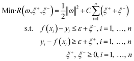
SVM is a supervised learning method used for classification and regression. It was introduced by Vapnik²⁸ and is successfully used for predicting values from very different fields. It has good generalization ability for regression and is suitable for finite sample regression problems. For a given training set T = (x_i, y_i), i = 1, …, l, the basic idea of the support vector regression machine is to select a suitable kernel function φ, to map the input variables (x_i) in low-dimensional space into higher-dimensional space, and represent the nonlinear problem in a linear form.^29,30where ω is the weight vector, and b is a constant, which are obtained by optimizing the following problem.where ξ⁺ and ξ⁻ are slack variables, and C is the penalty parameter for errors. For a more detailed description of SVM, the readers are referred to Wang et al.³¹

2.3 Particle swam optimization (PSO)

Particle Swam Optimization (PSO) was first proposed by Kennedy and Eberhart.³² It is proved to be effective for integer nonlinear optimization problems, continuous nonlinear optimization problems and combined optimization problems.^33–35 Inspired by the predation behavior of birds, PSO realizes the search for optimal solutions in complex space through cooperation and competition among individuals.³⁶ Each particle i, namely every individual of the swarm, remembers the best solution found by itself (P^ind) and by the whole swarm (P^glob). A particle moves along the search space at velocity V_i, and its position is denoted by P_i. The state of a particle is represented as follows.

V_i,d^(k+1) = ωV_i,d^k + c₁r₁(P^ind_i,d − P_i,d^k) + c₂r₂(P^glob_d − P_i,d^k) (5)

P_i,d^(k+1) = P_i,d^k + V_i,d^(k+1) (6)

where k denotes the iteration number, d represents the search direction, ω is the inertial weight, r₁ and r₂ are random numbers with uniform distribution in the range of 0 to 1, and c₁ and c₂ are the cognition and social parameters respectively. The PSO algorithm is well suited to handling nonlinear, nonconvex design spaces with discontinuities. It has the advantage of fast convergence and is robust.

2.4 Random forest algorithm (RF)

The RF algorithm is a supervised data-mining technique designed to produce accurate predictions without overfitting the data.^37,38 It is an ensemble of decision trees and uses both bootstrap aggregation (bagging) and random variable selection for tree building. During training, RF first creates a collection of regression trees, trains each tree on a bootstrapped sample of the original training data, and randomly selects potential predictors to determine the best split at each tree node. The bootstrapped sample for each tree is obtained by drawing a sample with replacement from the original training data. It has the same number of individuals as the original training data, but some individuals are repeated several times, while some others are left out (also called out-of-bag). The left-out individuals are used for estimation of the prediction error. For regression, the prediction output produced by each tree in the “forest” is summarized and processed by an averaging method.

2.5 Markov chain residual correction (MCRC)

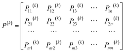
The core idea of the Markov method is to decide the state transferring probability matrix.^39,40 The transition probability of state E_i to state E_j after k iterations is determined as follows.where M_i indicates the total number of states, and m_ij^(k) is the number of times state E_i is transferred to state E_j. Then the n × m transfer matrix P^(k) is expressed as follows.

The state transition probability matrix is used to correct the original data by the Markov chain prediction model.

X^k = X⁰P^k (9)

where X^k is the probability transition matrix at time k, and X⁰ is the probability vector of the initial state. The prediction results are corrected according to the following formula.where F_g is the prediction value, and q is the boundary value of the original state interval.

3 Construction of the proposed GRA-PSO-SVM-RF-MCRC hybrid model for system reliability evaluation

In this section, the proposed hybrid chemical system reliability evaluation model is presented. The objective of the model is to obtain an accurate prediction for the reliability of a given chemical production system, by evaluating a collection of factors that impact different aspects of the system. Factors influencing the system reliability are collected according to the following five perspectives: man, machine, material, management and environment (4M1E).

3.1 4M1E aspects of chemical production systems

The reliability of industry production systems, especially chemical production systems, is affected by a collection of factors, covering the quality of raw materials (M) used, the state of the production machinery and instruments on-site (M), the comprehensive capacity of employees (Man, M), the supervision framework and organizational measures (M), and the overall production environment (E). One can conclude that the impact of the influential factors on the system reliability is highly nonlinear and mutually interfering, since each item listed above again contains a set of more detailed indicators and their influences on the system do not exist independently but rather are coupled with each other. Not to mention that the indicators are very likely to be measured by different means and therefore are of different dimensions. Owing to these factors, it is easy for prediction models to be stuck with a high level of inaccuracy and slow convergence. To tackle this, the influential factors are categorized into five perspectives: man, machine, material, management, and environment, in short 4M1E.

Firstly, man factors represent the comprehensive capacity of the system participants. The participants include decision makers, organizers, supervisors and direct operators. Examples of man factors are the direct operators’ technical ability, health condition, safety awareness, adaptability and manual operation capability, the supervisors’ and the inspectors’ understanding and mastery of the safety standards, etc. Secondly, machine, as an indispensable constituent of industrial production systems, affects the system reliability directly. Factors such as whether the equipment is in good condition for disaster prevention, whether the performance is stable, whether the machine is convenient and safe to operate, etc., will affect the reliability of the system. Thirdly, material refers to the hazardous, toxic, explosive and corrosive nature of the materials used in production. Fourthly, management mainly denotes the regulations that the organization enforces to regulate the daily operation of industrial production systems. Finally, environment defines the engineering and technical environment, such as the level of regional fire resistance, readily accessible safety facilities, level of noise, concentration of dust, and so on. The choice of specific indicators depends on the characteristics of the specific case at hand.

3.2 GRA-PSO-SVM-RF-MCRC hybrid model for system reliability prediction

The proposed approach realizes chemical system reliability evaluation in four steps. First, GRA is applied to evaluate the impact of each factor in system reliability in order to exclude those of low-impact. It is a decisive step towards ensuring model accuracy control and reducing the computational cost of machine learning methods when faced with complex industrial problems. Second, a hybrid PSO optimized SVM (PSO-SVM) model is used to evaluate the reliability of the five subsystems separately. Third, RF is used to correlate the reliability of the subsystems with that of the whole chemical production system. As stated by Zio,²⁴ it is very hard to acquire system reliability data with high quality. Usually, the collected data possess a high level of noise. Based on our previous research⁴¹ and literature survey, it is found that the randomness of the feature sampling of the RF algorithm enriches the diversity of the decision trees and thus prevents the model from overfitting and reduces the noise interference. Finally, Markov Chain Residual error Correction (MCRC) is used to improve the prediction accuracy. The evaluation process of the proposed approach is briefly illustrated in Fig. 1.

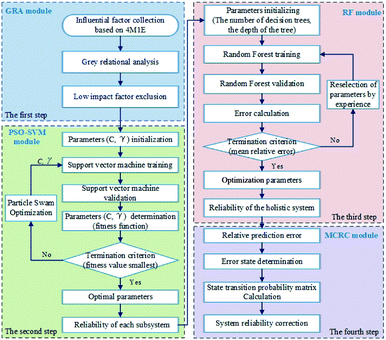Fig. 1 The proposed hybrid model (GRA-PSO-SVM-RF-MCRC) for the reliability evaluation of chemical production systems.

Considering the complicated interrelationships between various influential factors, GRA is used to trim the influential factors. After evaluating the influence that each factor has on the system reliability, factors with low impact are automatically excluded from the prediction process, thus improving the prediction accuracy and convergence speed. Subsequently, the remaining influential factors are evaluated and analyzed in groups to produce reliability evaluations for the respective subsystems, by using a combinatorial algorithm of SVM and PSO. SVM is chosen as the machine learning algorithm for reliability prediction of the five different subsystems because it is well-known to be a universal approximator of the majority of multivariate functions to the desired degree of accuracy.¹² As stated in Section 2.2, the selection of the kernel function is of great importance for ensuring the accuracy and universality of the proposed model. In the present study, the Radial Basis Function (RBF) is chosen as the kernel function for SVM regression,^29,30 which is formulated as follows.

where x is any point in space, x_i is the center of the kernel function, and σ is the function width parameter. During model training, PSO is used to carry out the optimization mechanism corresponding to the setting of the optimal kernel hyperparameters. Specifically, in order to improve model accuracy, γ and C (the penalty parameter for errors) are optimized; during the optimization procedure, the Mean Square Error (MSE) is used as the fitness function to assess the prediction accuracy of the model.

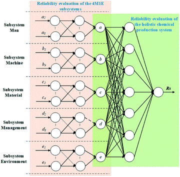
After the evaluation of the 4M1E subsystems, the predicted reliability values then serve as the input for the following step involving the reliability evaluation of the whole production system. Herein, RF is employed as the machine learning algorithm, and the output reliability evaluation value obtained in this step is then corrected by MCRC. The algorithm topology of the proposed evaluation framework is illustrated in Fig. 2.

Fig. 2 Topology of the proposed algorithm.

4 Case study: a synthetic ammonia plant

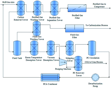
A real synthetic ammonia plant in China is taken as a test case in order to illustrate the applicability of the proposed method. Fig. 3 shows a flow chart of the ammonia plant. As is shown, the ammonia synthesis process consists of 15 units, including carbon removal, purified gas separation, flashing, desorption, condensation and so on. For the reliability evaluation of the process, 37 indicators that reflect the performance of the five considered aspects in accordance with the categorization explained in Section 3.1 are collected. For the man subsystem, eight influential factors were considered in the present study, which are listed in Table 1. Nine indicators were considered for the evaluation of the machine subsystem, which are denoted by b_i and listed in Table 2. As for the material subsystem, in the context of chemical production, reaction temperature and pressure are also taken into consideration. The material factors considered are denoted by c_i, and are listed in Table 3, while the considered items related to the management perspective are listed in Table 4. Lastly, the environmental effect is complex and changeable. In the current case, factors such as regional fire resistance level and environmental noise level are taken into consideration. Table 5 lists the detailed items related to the environment subsystem. The specific values collected for these indicators are given in Table 6. As is shown, 100 data entries in total were collected periodically from the ammonia plant over one year. This data set was also used in the study by Liu et al.²¹

Fig. 3 Flow chart for the considered ammonia plant.

Table 1 Considered reliability factors from the man subsystem

Symbol	Meaning	Symbol	Meaning
a1	Average age	a5	Safety knowledge
a2	Average working age	a6	Safety consciousness
a3	Education degree	a7	Health condition
a4	Vocational safety training degree	a8	Ratio of senior engineers

---

Table 2 Considered reliability factors from the machine subsystem

Symbol	Meaning	Symbol	Meaning
b1	Equipment protector intact rate	b6	Communication facility intact rate
b2	Equipment intact rate	b7	Anti-static facility intact rate
b3	Fire facility intact rate	b8	Transport line intact rate
b4	Alarm facility intact rate	b9	Emergency rescue facility timeliness
b5	Monitor intact rate

---

Table 3 Considered reliability factors from the material subsystem

Symbol	Meaning	Symbol	Meaning
c1	Material fire hazard	c4	Material corrosivity
c2	Material toxicity	c5	Reaction temperature
c3	Material explosiveness	c6	Reaction pressure

---

Table 4 Considered reliability factors from the management subsystem

Symbol	Meaning	Symbol	Meaning
d1	Management organization	d5	Protector management regulations
d2	Safe operation regulations	d6	Equipment safety management regulations
d3	Safety inspection regulations	d7	Hazard management regulations
d4	Fire and explosion protection regulations	d8	Safe accident treatment regulations

---

Table 5 Considered reliability factors from the environment subsystem

Symbol	Meaning	Symbol	Meaning
e1	Regional fire resistance level	e4	Operation ground slip resistance
e2	Environmental noise level	e5	Dust concentration
e3	Material placement level	e6	Regional safe passage distance

---

Table 6 Collected system reliability datasets for the case study^a

No.	a1	⋯	a8	a	b1	⋯	b9	b	c1	⋯	c6	c	d1	⋯	d8	d	e1	⋯	e6	e	Rs
a a, b, c, d and e represent the reliability of the five subsystems. Their specific values are obtained by the Delphi method. The rows present the time series data set periodically collected from the ammonia production plant over one year.
1	37.1	⋯	28.2	4.78	98.3	⋯	92.4	4.96	1	⋯	14.9	4.98	0.8	⋯	1	1.08	0.8	⋯	82	2.78	3.83
2	23.9	⋯	5.1	1.02	97.7	⋯	94.7	4.89	1	⋯	14.9	4.85	1.7	⋯	2.8	2.77	0.5	⋯	103	1.12	3.86
3	22.3	⋯	17.9	3.04	89.8	⋯	86.1	3.97	0.9	⋯	14.9	3.99	4.2	⋯	4.1	4.34	0.7	⋯	83	1.98	4.06
4	33.1	⋯	23.1	4.12	90.2	⋯	87.4	4.09	0.9	⋯	14.9	4.07	4.1	⋯	4.3	3.56	1	⋯	57	4.89	4.54
5	27.1	⋯	7.9	1.96	92.3	⋯	73.3	1.05	0.5	⋯	17	1.08	1.5	⋯	1.8	1.65	0.8	⋯	78	2.89	1.45
⋯	⋯	⋯	⋯	⋯	⋯	⋯	⋯	⋯	⋯	⋯	⋯	⋯	⋯	⋯	⋯	⋯	⋯	⋯	⋯	⋯	⋯
96	33.1	⋯	24.3	4.19	98	⋯	94.8	4.96	0.5	⋯	18	1.08	0.8	⋯	1	1.12	0.8	⋯	78	2.90	3.27
97	33.1	⋯	23.7	4.09	97.8	⋯	92.2	4.91	0.5	⋯	17	1.11	1	⋯	1.1	1.11	0.9	⋯	63	4.01	3.14
98	21.8	⋯	16.8	2.82	85.8	⋯	71.9	1.09	0.9	⋯	14.9	4.02	4	⋯	4.3	4.54	1	⋯	56	4.8	3.12
99	23.9	⋯	4.5	1.05	84.8	⋯	82.2	2.42	0.5	⋯	18	1.07	3.2	⋯	2.5	2.50	0.5	⋯	102	1.16	2.96
100	35.2	⋯	25.8	4.85	67.9	⋯	80.7	2.41	0.5	⋯	18	1.16	4.2	⋯	4.3	4.22	0.8	⋯	78	2.92	3.24

---

It is worth mentioning that, in this study, the system reliability is evaluated at five levels, ranging from the most unreliable to the most reliable, which are given in Table 7. The values of the indicators listed in Tables 1–5 were collected from the ammonia plant. The readily available system information, such as the average age and education degree of the workers, was directly collected from the information system of the plant. For other non-quantitative indexes, for which the specific values are not readily available, the Delphi method⁴² was employed to quantify their reliability levels. For example, the safety knowledge of the operating engineers (a₅) and the fire hazard level of the raw materials (c₁) are indicators that cannot be easily quantified by precise analytical models. Hence, they are characterized by five common grades, namely, 1, 0.9, 0.8, 0.7 and 0.5.¹⁹ Here, 1 represents the best state, 0.9 represents a good state, 0.8 represents a general state, 0.7 represents a poor state, and 0.5 represents the worst state. Generally speaking, if the system reliability is evaluated to be greater than 3 (out of 5), it can be considered safe and does not require maintenance.

Table 7 Five levels of system reliability

Level	1	2	3	4	5
Reliability	Unreliable	Less reliable	Generally reliable	More reliable	Very reliable

---

The Delphi method is a forecasting tool originally developed by Norman Dalkey from the RAND Corporation for a U.S. military project in the 1950s, and has been extensively studied and reviewed since then. It is characterized by the following four key features: (1) anonymity of Delphi participants, which allows the participants to express opinions freely and make decisions based on their own merit; (2) iteration, which allows the participants to refine their view iteratively in light of the progress of the group work; (3) controlled feedback, which allows the participants to be informed of the other participants’ perspectives and provides them the opportunity to clarify or change their views; (4) statistical aggregation of group responses, which allows quantitative analysis and data interpretation.⁴³ For more information about this method, readers are referred to this publication.⁴⁴ The Delphi method can be applied to problems where there is incomplete knowledge, or problems that do not lend themselves to precise analytical techniques but rather could benefit from the subjective judgments of individuals on a collective basis.⁴² The merits of the Delphi method are well suited to the needs of this study.

5 Results and discussion

5.1 Grey relational analysis (GRA)

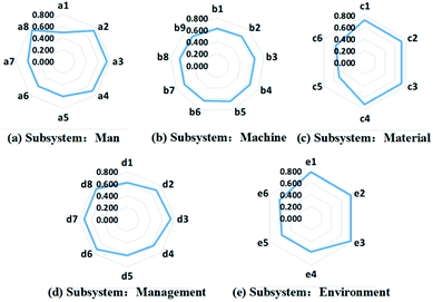
tAfter GRA of each subsystem, the degrees of correlation between each considered influential factor and the reliability of the respective subsystem are obtained. The analysis results of the five subsystems are illustrated in the form of radar charts, which are shown in Fig. 4. For the man subsystem, the average age of the employees (a₁) does not affect the system reliability significantly compared to the other four principal influential factors, namely, the average working age (a₂), education degree (a₃) and vocational safety training degree (a₄) of the employees and the ratio of senior engineers in the workforce (a₈). The same conclusions apply for the safety knowledge (a₅), safety consciousness (a₆) and health condition of the workers (a₇). As a result, the four correlation factors with low impact, i.e. a₁, a₅, a₆ and a₇, are excluded from the system reliability evaluation. For the machine subsystem, as shown in Fig. 4(b), the nine considered factors are of equal importance for the system reliability assessment, thus all of these factors are included in the evaluation model. As for the material subsystem, it can be concluded from Fig. 4(c) that four of the selected factors have a non-negligible influence on the system reliability, therefore, the remaining two factors, which refer to the reaction temperature (c₅) and pressure (c₆), are left out during the reliability assessment of the subsystem. The GRA result for the management subsystem is presented in Fig. 4(d), which suggests that regulations for safe operation (d₂), safety inspection (d₃), equipment safety management (d₆), hazard management (d₇) and safe accident treatment (d₈) impact the system reliability more than the other three indicators. Consequently, only these five indicators are considered in the subsequent assessment model. Last but not least, three indicators out of six were confirmed by the grey relational analysis for the environment subsystem, as can be concluded from Fig. 4(e). In this way, the 37 influential factors selected for system reliability evaluation are reduced to 25, each of which is considered to be strongly correlated with the reliability of the respective subsystems.

Fig. 4 Radar charts illustrating the Gray Relational Analysis (GRA) results for the correlation degrees of the relative influential factors in: (a) man subsystem, (b) machine subsystem, (c) material subsystem, (d) management subsystem, and (d) environment subsystem.

5.2 Prediction results for the system reliability by applying the proposed two-step hybrid algorithm

After the GRA procedure, the remaining 25 influential factors were processed by the proposed hybrid algorithm. To better balance the datasets for the training and validation of the two evaluation models, the collected 100 datasets were first divided into two groups. The first 50 (50%) datasets were used as training data to train the PSO-SVM models to evaluate the reliability of the subsystems. After 200 generations of evolution, the evaluation models for the five subsystems were obtained.

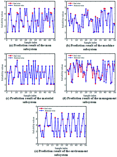
The fitness curves of the evaluation model training for each subsystem are shown in Fig. 5. It can be seen that, after the first 30 iterations of model training, the models all reached a high fitness. Then, the remaining 50 (50%) datasets were used as testing data for the trained models to produce predictions for the subsystem reliability. A comparison between the predicted reliability value and the actual value for each subsystem is given in Fig. 6. It can be concluded from the results that the reliability prediction for the respective subsystems has reached a satisfactory accuracy.

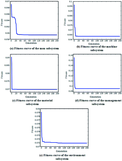Fig. 5 Fitness curves of the evaluation model training for: (a) man subsystem, (b) machine subsystem, (c) material subsystem, (d) management subsystem, and (d) environment subsystem.

Fig. 6 Comparison of the reliability values predicted by the obtained PSO-SVM model and the actual values for: (a) man subsystem, (b) machine subsystem, (c) material subsystem, (d) management subsystem, and (d) environment subsystem.

After the model training for the subsystems, the predictive results from the trained PSO-SVM models for the subsystems were used to develop a reliability evaluation model for the overall ammonia production plant. Namely, the 50 predicted reliability values for each subsystem were the input for the RF model to correlate the reliability of the five subsystems with that of the whole production system. Since the 50 datasets were obtained from the 51^st to the 100^th data entries of the original dataset, they were labelled as No. 51^pred to No. 100^pred. Then, 80% of the dataset (i.e. No. 51^pred to No. 90^pred) was used as the training set, and the remaining 20% (i.e. No. 91^pred to No. 100^pred) was used as the testing set for the RF model.

In order to better assess the efficacy of the proposed method, a comparison between the proposed model and the model developed by Liu et al.²¹ was carried out, and is given in Table 8. As shown in Table 8, the relative error of the prediction by the proposed model varies in the range of 0 to 11.2%, while that of the literature result varies between 0 and 23.3%. The relative errors of the two models are visualized in Fig. 7. This suggests that the proposed approach is more stable and accurate in the prediction of system reliability.

Table 8 Comparison of the reliability predictions for the ammonia plant between the proposed model and the model developed by Liu et al.^21a

No.	R^acts	Model developed by Liu et al.^21			The proposed approach
		R^preds	Absolute error	Relative error (%)	R^preds	Absolute error	Relative error (%)
a R^acts – actual value of system reliability, R^preds – predicted value of system reliability.
91^pred	2.68	2.16	−0.5205	−19.42	2.53	−0.1480	−5.52
92^pred	3.48	2.95	−0.5261	−15.12	3.13	−0.3469	−9.97
93^pred	3.57	3.29	−0.2773	−7.77	3.34	−0.2346	−6.57
94^pred	3.80	3.96	0.1603	4.22	3.45	−0.3523	−9.27
95^pred	2.72	2.36	−0.3635	−13.36	2.62	−0.1001	−3.68
96^pred	3.27	3.11	−0.1560	−4.77	3.10	−0.1687	−5.16
97^pred	3.14	3.16	0.0236	0.75	3.20	0.0584	1.86
98^pred	3.12	3.79	0.6721	21.54	3.47	0.3495	11.20
99^pred	2.96	2.27	−0.6897	−23.30	2.67	−0.2914	−9.85
100^pred	3.24	3.47	0.2349	7.25	3.20	−0.0370	−1.14

---

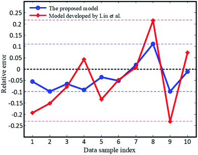Fig. 7 Relative prediction errors of the proposed model and the model developed by Liu et al.²¹

To further analyze the prediction results and compare the proposed approach with the literature method, the Mean Square Error (MSE) and the Mean Relative Error (MRE) were calculated to assess the results of each evaluation step, according to the following formulas.

where k_i is the actual value, o_i is the predicted value, and N is the total number of datasets. Table 9 lists the analysis results for the method developed by Liu et al.,²¹ while the results for the proposed model are shown in Table 10.

Table 9 Prediction accuracy analysis for the subsystems and the overall system for the method developed by Liu et al.^21a

Category	Step-1					Step-2
	R^man	R^mach	R^mat	R^mana	R^env	Rs
a R^man, R^mach, R^mat, R^mana, R^env and Rs denote the system reliability of the five subsystems, namely, man, machine, material, management and environment, and the overall system, respectively.
MSE	0.015	0.160	0.030	0.202	0.017	0.179
MRE	4.62%	9.57%	6.00%	14.37%	4.07%	11.75%

---

Table 10 Prediction accuracy analysis for the subsystems and the overall system for the proposed model

Category	Step-1					Step-2
	R^man	R^mach	R^mat	R^mana	R^env	Rs
MSE	0.018	0.021	0.007	0.217	0.007	0.057
MRE	3.97%	4.12%	2.81%	13.40%	2.75%	6.42%

---

It can be concluded from Tables 9 and 10 that the prediction results of the proposed approach are more accurate than those of the model developed by Liu et al.²¹ In terms of MSE, the proposed model achieves predictions with 0.057 deviation from the true value of the overall system reliability, which is much lower than the deviation observed for the literature method, 0.179. In terms of MRE, the deviation observed for the proposed model is 6.42%, while that for the literature model is 11.75%. The same situation occurred for the prediction of the five subsystems.

5.3 Results of Markov chain residual correction

It is shown that the proposed model gives relatively accurate predictions for system reliability, with relative errors within 10%. In order to further improve the prediction accuracy and enhance the model stability, Markov chain residual correction is applied.

In this study, the golden ratio is applied to divide the Markov chain states into intervals, based on the relative prediction errors for the training sets as listed in Table 11. The division point γ_r is determined by the following equation.

γ_r = Ω^sX̃ |s| < t, r = 1, 2, …, t (14)

where X̃ is the mean value of the relative prediction error X, Ω is the golden partition ratio, which equals 0.618, and s and the magnitude number t are determined based on the range of the relative prediction error X. By assigning values of 1 and −1 to s, three state intervals were obtained, namely, E₁[0, 0.182], E₂[0.182, 0.475] and E₃[0.475, 1], which correspond to the original state intervals, , and .

Table 11 Factors of the man subsystem

No.	Actual value	Predicted value	Relative error (%)	Normalized value (%)	State
51^pred	3.09	3.07	−0.50	24.62	E2
52^pred	2.99	2.97	−0.66	24.21	E2
53^pred	3.12	2.88	−7.80	6.69	E1
⋯	⋯	⋯	⋯	⋯	⋯
88^pred	3.59	3.50	−2.42	19.91	E2
89^pred	2.67	2.82	5.76	39.97	E2
90^pred	3.99	3.64	−8.69	4.50	E1

---

After the determination of state intervals, the transition matrix P is obtained for each data set. Taking the second data entry in Table 8 as an example, its state transition matrix P is calculated as follows.

The state vector of the initial state is given as (1, 0, 0). Multiplying the state vector by the state transition matrix produces its state vector (0.2, 0.5, 0.3). According to the division of the state intervals, the relative error is in the state range E₂. Hence, improved prediction results are achieved by MCRC, as shown in Table 12.

Table 12 Comparison between the original predicted value and the value corrected by the Markov chain residual correction

Actual value	Original predicted value		Corrected value from the Markov chain residual correction
	Predicted value	Relative error (%)	Modified value	Relative error (%)
3.48	3.13	−9.97	3.23	−7.18

---

By applying the MCRC to all the system prediction datasets, the prediction accuracy of the evaluation model is further improved. For the proposed model, the MSE is reduced from 0.057 to 0.022, and the MRE drops from 6.42% to 3.77%. It is worth mentioning that the MCRC method was also applied to the literature method,²¹ which resulted in a decrease in the MSE from 0.179 to 0.131, and the MRE from 11.75% to 9.69%. A comparison of the prediction accuracy after MCRC between the two models is presented in Table 13. This proves that the MCRC methodology can be used to effectively reduce the amplitude of the prediction error. This is due to the fact that the Markov chain uses the transfer matrix to analyze the future trend of the current status.

Table 13 Comparison of prediction accuracy between the two models

Model	MSE	MRE (%)
Model developed by Liu et al.^21	0.131	9.69
The proposed model	0.022	3.77

---

6 Conclusion

This paper presents a hybrid reliability prediction model for chemical production systems, striving to deliver satisfactory predictive reliability results for chemical production systems by combining the advantages of machine learning algorithms. First, factors affecting the reliability of chemical production systems are collected from five perspectives, namely man, machine, material, management and environment (4M1E), followed by a GRA analysis procedure on each subsystem, in order to reduce the dimension of the problem at hand and thus speed up the convergence rate. Second, support vector regression is applied to predict the reliability of the five perspectives separately, and PSO is used to optimize the parameters involved. Third, the RF algorithm is employed to predict the reliability of the whole chemical production system. Lastly, MCRC is adopted to further improve the prediction accuracy. Applying the model to an ammonia plant in China proved its efficacy. Compared to the literature method, the proposed model achieved better prediction results with lower prediction error. Both the Mean Square Error (MSE) and the Mean Relative Error (MRE) were calculated in order to evaluate the prediction accuracy of the proposed model. It is shown that, in terms of MSE, the proposed model achieved predictions with 0.022 deviation from the true value of the overall system reliability, which is much lower than the deviation observed for the literature method, 0.131. In terms of MRE, the deviation observed for the proposed model is 3.77%, while that for the literature model is 9.69%. Furthermore, it is concluded that the MCRC methodology can be used to effectively reduce the amplitude of the prediction error, due to the fact that the Markov chain uses the transfer matrix to analyze the future trend of the current status. In addition, the proposed model can be extended to the reliability evaluation of other complex industrial production systems.

The comparison between the proposed method and Liu’s work²¹ proved that PSO-SVM and RF can better deal with the scarcity of available reliability data, as the training process for GA-BP requires more data to ensure model accuracy. Additionally, it should be noted that the proposed approach is a machine learning method based on collected industrial data. Although selection of more suitable machine learning methods can certainly improve evaluation accuracy, the whole modeling and evaluation process is founded on the quality of the training data. If the model is provided with better quality data, then better result accuracy can be achieved. Also, as randomness exists in the machine learning process (for example, the randomness of the feature sampling of RF), uncertainties exist in the model training and estimation. When the same model is trained at a different time and/or on a different machine, the result might be slightly different.

Conflicts of interest

There are no conflicts to declare.

Acknowledgements

The financial support for the project from the National Natural Science Foundation of China (21776183), and the Fundamental Research Funds for the Central Universities (YJ201838) is gratefully acknowledged.

Notes and references

1. H. Wu and J. Zhao, Comput. Chem. Eng., 2018, 115, 185–197.
2. Z. Zhang and J. Zhao, Comput. Chem. Eng., 2017, 107, 395–407.
3. T. Kongsvik, G. Gjøsund and K. M. Vikland, Saf. Sci., 2016, 81, 81–89.
4. Y. Wang, M. Tian, D. Wang, Q. Zhao, S. Shan and S. Lin, Procedia Eng., 2012, 45, 231–234.
5. B. S. Dhillon and S. N. Rayapati, IEEE Trans. Reliab., 1988, 37, 199–208.
6. N. Sadou and H. Demmou, Reliab. Eng. Syst. Safe., 2009, 94, 1848–1861.
7. T. T. Pham, T.-C. Kuo and D. M. Bui, Int. J. Electr. Power Energy Syst., 2020, 118, 105786.
8. H. Soltanali, A. Rohani, M. Tabasizadeh, M. H. Abbaspour-Fard and A. Parida, Quality Technology & Quantitative Management, 2020, 17, 186–202.
9. C. L. Hwang, F. A. Tillman and M. H. Lee, IEEE Trans. Reliab., 1981, R–30, 416–423.
10. D. F. Rudd, Ind. Eng. Chem. Fundam., 1962, 1, 138–143.
11. F. A. Tillman, W. Kuo, C. L. Hwang and D. L. Grosh, IEEE Trans. Reliab., 1982, R–31, 362–372.
12. P. J. G. Nieto, E. García-Gonzalo, F. S. Lasheras and F. J. de Cos Juez, Reliab. Eng. Syst. Safe., 2015, 138, 219–231.
13. Z. Wei, T. Tao, D. ZhuoShu and E. Zio, Reliab. Eng. Syst. Safe., 2013, 119, 109–116.
14. T. Tao, E. Zio and W. Zhao, Reliab. Eng. Syst. Safe., 2018, 177, 35–49.
15. R. He, Y. Dai, J. Lu and C. Mou, Reliab. Eng. Syst. Safe., 2018, 180, 385–393.
16. N.-C. Xiao, M. J. Zuo and C. Zhou, Reliab. Eng. Syst. Safe., 2018, 169, 330–338.
17. M. Menz, C. Gogu, S. Dubreuil, N. Bartoli and J. Morio, Reliab. Eng. Syst. Safe., 2020, 196, 106771.
18. Z. Wang and A. Shafieezadeh, Reliab. Eng. Syst. Safe., 2020, 195, 106735.
19. W. Liu, M. Chen and X. Ji, China Saf. Sci. J., 2015, 25, 139–144.
20. Y. Miao, R. Kang and X. Chen, IOP Conf. Ser.: Mater. Sci. Eng., 2017, 274, 012004.
21. W. Liu, K. Wei, J. Xu and X. Ji, Qual. Reliab. Eng. Int., 2017, 33, 1337–1349.
22. L. Luo, F. Cheng, T. Qiu and J. Zhao, Comput. Chem. Eng., 2017, 106, 1–16.
23. M. Yihua and X. Tuo, Syst. Eng. Procedia, 2011, 1, 213–220.
24. E. Zio, Reliab. Eng. Syst. Safe., 2009, 94, 125–141.
25. J. Deng, Syst. Contr. Lett., 1982, 1, 288–294.
26. E. Granada, J. Morán, J. L. Míguez and J. Porteiro, Fuel Process. Technol., 2006, 87, 123–127.
27. Y. Kuo, T. Yang and G.-W. Huang, Comput. Ind. Eng., 2008, 55, 80–93.
28. V. N. Vapnik, The Nature of Statistical Learning Theory, Springer Science+Business Media, LLC, New York, 1st edn, 1995.
29. J. Li, C. Zhao, W. Huang, C. Zhang and Y. Peng, Anal. Methods, 2014, 6, 2170–2180.
30. J. Zhang, J. Wu, L. Tang, J. Jiang, G. Shen and R. Yu, Anal. Methods, 2015, 7, 5108–5113.
31. X. Wang, D. Luo, X. Zhao and Z. Sun, Energy, 2018, 152, 539–548.
32. J. Kennedy and R. Eberhart, Proceedings of IEEE International Conference on Neural Networks, 1995, vol. 4, pp. 1942–1948.
33. L. D. S. Coelho and C. A. Sierakowski, Adv. Eng. Softw., 2008, 39, 877–887.
34. S. Suresh, P. B. Sujit and A. K. Rao, Compos. Struct., 2007, 81, 598–605.
35. K. E. Parsopoulos and M. N. Vrahatis, Nat. Comput., 2002, 1, 235–306.
36. Y. Shi and R. C. Eberhart, Proceedings of the 1999 Congress on Evolutionary Computation, 1999, vol. 3, pp. 1945–1950.
37. L. Breiman, Mach. Learn., 2001, 45, 5–32.
38. L. R. Iverson, A. M. Prasad, S. N. Matthews and M. Peters, For. Ecol. Manage., 2008, 254, 390–406.
39. E. Hatzipantelis, A. Murray and J. Penman, Artificial Neural Networks, 1995, vol. 409, pp. 369–374.
40. A. Dahamsheh and H. Aksoy, Arabian J. Sci. Eng., 2014, 39, 2513–2524.
41. C. Chen, L. Zhou, X. Ji, G. He, Y. Dai and Y. Dang, Ind. Eng. Chem. Res., 2020 DOI:10.1021/acs.iecr.0c01409.
42. G. J. Skulmoski, F. T. Hartman and J. Krahn, Journal of Information Technology Education: Research, 2007, 6, 1–21.
43. G. Rowe and G. Wright, Int. J. Forecast., 1999, 15, 353–375.
44. N. Dalkey, Futures, 1969, 1, 408–426.

---

Footnote

† Electronic supplementary information (ESI) available. See DOI: 10.1039/c9ra09654j

---