 Open Access Article
Improved method of structure-based virtual screening based on ensemble learning†
Jin Li ab,
WeiChao Liub,
Yongping Songc and
JiYi Xia
 *b
*b
aCollege of Computer and Information Science, Southwest University, Chongqing 400715, China
bKey Laboratory of Medical Electrophysiology of Ministry of Education, Medical Electrophysiological Key Laboratory of Sichuan Province, Institute of Cardiovascular Research, School of Medical Information and Engineering, Southwest Medical University, Luzhou 646000, China. E-mail: jiyixia@swmu.edu.cn
cLuzhou High School, Luzhou 646000, China
First published on 19th February 2020
Abstract
Virtual screening has become a successful alternative and complementary technique to experimental high-throughput screening technologies for drug design. Since the scoring function of docking software cannot predict binding affinity accurately, how to improve the hit rate remains a common issue in structure-based virtual screening. This paper proposed a target-specific virtual screening method based on ensemble learning named ENS-VS. In this method, protein–ligand interaction energy terms and structure vectors of the ligands were used as a combination descriptor. Support vector machine, decision tree and Fisher linear discriminant classifiers were integrated into ENS-VS for predicting the activity of the compounds. The results showed that the enrichment factor (EF) 1% of ENS-VS was 6 times higher than that of Autodock vina. Compared with the newest virtual screening method SIEVE-Score, the mean EF 1% and AUC of ENS-VS (mean EF 1% = 52.77, AUC = 0.982) were statistically significantly higher than those of SIEVE-Score (mean EF 1% = 42.64, AUC = 0.912) on DUD-E datasets; and the mean EF 1% and AUC of ENS-VS (mean EF 1% = 29.73, AUC = 0.793) were also higher than those of SIEVE-Score (mean EF 1% = 25.56, AUC = 0.765) on eight DEKOIS datasets. ENS-VS also showed significant improvements compared with other similar research. The source code is available at https://github.com/eddyblue/ENS-VS.
1. Introduction
Virtual screening (VS) is a computational approach used to identify active compounds by predicting their activity. In recent years, it has become a successful alternative and complementary technique to experimental high-throughput screening technologies for drug design, because of its ability to decrease the cost and increase the hit rate of screening greatly.1–4 Technically, virtual screening can be categorized into two types, namely, ligand-based virtual screening (LBVS) and structure-based virtual screening (SBVS). The similarity principle is used to identify potentially active compounds based on their similarity to known reference ligands in LBVS. This can be done by a variety of methods, including similarity and substructure searching,5 pharmacophore matching6 or 3D shape matching.7 SBVS predicts the active compounds with higher docking quality by involving explicit molecular docking of each ligand into the binding site of the target. Many docking tools are used in SBVS, such as Glide,8 GOLD,9 Autodock,10 and Autodock vina (refer to as Vina).11 Because SBVS is based on the physical interactions between the protein target and the ligands, whereas LBVS is based on the similarity of known active compounds, SBVS is more likely to obtain novel compounds than LBVS. Another advantage of SBVS is the ability to perform interaction analysis to understand the affinity and selectivity of the compounds by using the docked structures.However, the classical scoring functions implemented in the docking software usually use simple function form and the linear regression method, which leads to the binding affinity between the target and the compound not being predicted accurately. Therefore, how to increase the hit rate becomes one of the most challenging tasks in SBVS.
In recent years, researchers have applied machine learning methods12 to improve the performance of VS and achieved good results, such as support vector machine (SVM), decision tree, neural network, deep-learning, etc.13–16 Unlike the classical scoring functions with assumed mathematical functional form, machine learning-based scoring functions implicitly learn the relationships among protein–ligand complexes by non-linear regression.17 However, it is hard to achieve high accuracy by one learner, the emergence of ensemble learning such as bagging,18 boosting18,19 and random forest,20–22 can gain better accuracy.
Moreover, it has been widely accepted that target-specific scoring functions may achieve better performance compared with universal scoring functions in actual drug research and development processes.23,24 Therefore, we intended to build a target-specific VS model based on ensemble learning. In this model, we treated the ligand activity labelling task as a classification problem.
Feature selection is one of the most important factors affecting the performance of machine learning methods. In the past, two types of descriptors (features for the active and non-active compounds classification) were usually used to describe the features of active and non-active compounds. One is protein–ligand interaction energy terms16,25 which have no enough predictive power, since it is relatively too simple. The other is molecular fingerprint26–28 which is prone to the overfitting due to too many descriptors. Therefore, we propose our first scientific question: How do we choose such descriptors that can effectively distinguish active compounds from non-active ones?
Virtual screening aims to distinguish active compounds from a large number of non-active compounds. However, it will result in high recall and low precision12 due to the serious imbalanced numbers of active and non-active compounds in current commonly used training data.29,30 Previous studies13,31,32 usually use random under-sampling to solve this problem, but it is easy to lose the important information of the non-active compounds. Therefore, we propose our second scientific question: How do we effectively utilize the information of imbalanced data?
On the other hand, since most of the previous studies13,16,33,34 just use only one machine learning algorithm for classification, such as SVM35 and neural network;36 and the ensemble learning methods only use one base learner.18,19 One type of learner may not work well for most targets. For this reason, we propose our third scientific question: Can we integrate more machine learning algorithms and build a stable model which is suitable for most targets?
According to these aforementioned scientific questions, we present a target-specific virtual screening method based on ensemble learning named ENS-VS, which has the following three innovations.
Firstly, we select a moderate number of descriptors to classify the active and non-active compounds by considering both protein–ligand interaction energy terms and the structure character of the ligand.
Secondly, we develop a method to solve the data imbalanced problem based on previously well-developed sampling ensemble method.37,38
Finally, an ensemble learning approach is developed by integrating the SVM,35 decision tree39 and Fisher linear discriminant (refer to as Fisher)40 algorithms to improve the predictive accuracy.
2. Materials and methods
2.1 Materials
The Directory of Useful Decoys, Enhanced (DUD-E)29 database was used to evaluate the performance of ENS-VS. DUD-E contains 102 targets. All targets have two types of ligands: actives (active compounds) and decoys (non-active compounds), which can be labelled as 1 and −1 for classification model training. Since the decoys are similar in physico-chemical properties to the actives but different in their chemical structures, the datasets are more reliable for testing virtual screening method. The number of decoys is much larger than that of actives. If the number of the actives for model training is too small, it cannot sufficiently represent the distribution of the positive data. And if the samples is less than the number of the features in machine-learning model, the risk of overfitting will be high. In our method, the number of the features is more than one hundred. For this reason, we selected 37 targets with more than 200 actives to build 37 target-specific models by ENS-VS. 12 out of 37 targets that cover a wide range of popular drug targets were selected to show the detail information, which contain 3 proteases, 2 nuclear receptors, 3 kinases, 2 GPCR, and 2 other target families. The initial number of actives, decoys and the protein targets used for model training are listed in Table 1.| Familya | Protein | PDB | Activesb | Decoysc |
|---|---|---|---|---|
| a Protein family classification of selected protein targets.b Number of actives collected from DUD-E.c Number of decoys collected from DUD-E. | ||||
| Protease | try1 | 2ayw | 449 | 25![[thin space (1/6-em)]](https://www.rsc.org/images/entities/char_2009.gif) 980 980 |
| Protease | thrb | 1ype | 461 | 27![[thin space (1/6-em)]](https://www.rsc.org/images/entities/char_2009.gif) 004 004 |
| Protease | bace1 | 3l5d | 283 | 18![[thin space (1/6-em)]](https://www.rsc.org/images/entities/char_2009.gif) 100 100 |
| Nuclear | esr1 | 1sj0 | 383 | 20![[thin space (1/6-em)]](https://www.rsc.org/images/entities/char_2009.gif) 685 685 |
| Nuclear | ppara | 2p54 | 373 | 19![[thin space (1/6-em)]](https://www.rsc.org/images/entities/char_2009.gif) 339 339 |
| Kinase | src | 3el8 | 524 | 34![[thin space (1/6-em)]](https://www.rsc.org/images/entities/char_2009.gif) 500 500 |
| Kinase | egfr | 2rgp | 542 | 25![[thin space (1/6-em)]](https://www.rsc.org/images/entities/char_2009.gif) 050 050 |
| Kinase | vgfr2 | 2p2i | 409 | 24![[thin space (1/6-em)]](https://www.rsc.org/images/entities/char_2009.gif) 950 950 |
| GPCR | aa2ar | 3eml | 482 | 31![[thin space (1/6-em)]](https://www.rsc.org/images/entities/char_2009.gif) 550 550 |
| GPCR | adrb1 | 2vt4 | 247 | 15![[thin space (1/6-em)]](https://www.rsc.org/images/entities/char_2009.gif) 850 850 |
| Others | hivrt | 3lan | 338 | 18![[thin space (1/6-em)]](https://www.rsc.org/images/entities/char_2009.gif) 891 891 |
| Others | pgh2 | 3ln1 | 435 | 23![[thin space (1/6-em)]](https://www.rsc.org/images/entities/char_2009.gif) 150 150 |
The DEKOIS 2.0 database41 was used as an independent test set. The active compounds of DEKOIS were collected from ChEMBL database. The decoy compounds were generated from the ZINC database, regarding high physicochemical similarity between actives and decoys and avoidance of potentially active compounds. In this evaluation, the ligands in DEKOIS datasets were used for testing the model trained by DUD-E datasets. Eight DEKOIS2.0 targets with more than 200 actives in DUD-E were selected for the test: aa2ar (a2a), aces (ache), adrb2 (adrb2), akt1 (akt1), fa10 (fxa), egfr (egfr), hivrt (hiv1rt) and ppara (ppara). The former names and the latter names in the brackets were used in DUD-E and DEKOIS datasets, respectively. Structurally similar compounds (similarity ≥ 0.8) between training data and test data were excluded from training set.
2.2 Workflow
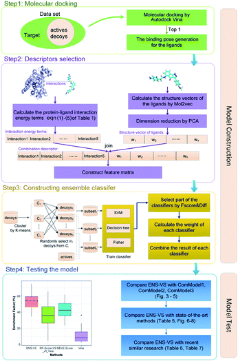
The workflow of ENS-VS development is shown in Fig. 1. The generic workflow includes the following steps: (i) dock all the actives and decoys into the binding pocket of the target and select the best pose of the ligands ranked by Autodock vina (step 1 of Fig. 1); (ii) calculate the five protein–ligand interaction energy terms and the structure vector representation of the ligands; and then create the feature matrix (step 2 of Fig. 1); (iii) train the ensemble classifier on the training set; and tune the hyperparameter based on the validation dataset (step 3 of Fig. 1); (iv) test the model by the test set and calculate performance metrics (step 4 of Fig. 1).2.3 Molecular docking
The generic process for docking simulation includes the following steps: (i) prepare proteins and ligands by adding hydrogens but merging non-polar hydrogens and removing water molecules. (ii) Convert the PDB files of the protein and the mol2 files of ligands into PDBQT formats by the python script prepare_protein4.py and prepare_ligand4.py in MGLTools.42 (iii) Dock the actives and decoys to their target by Autodock vina.43 The grid box is set to 20 × 20 × 20 with the center of the crystal ligand, and num_modes is set to 1. The num_modes is used to set the maximum number of binding modes generated by Vina. The binding modes are sorted by the scoring function of Vina. Here, we only obtain the top scoring binding mode. The rest of parameters are assigned default values. (v) The top scoring conformation will be obtained as the optimal binding mode of the ligand (step 1 of Fig. 1).2.4 Descriptors selection
We used a combination descriptors including interaction energy terms and ligand features. Fergus et al. 44 combined 1D or 2D fingerprint as ligand features to improve the machine learning scoring functions which are used protein–ligand interactions as features. Their method achieved good results. But these ligand features were conformation independent. Therefore, we intended to integrate ligand features which can describe the 3D structures of the ligands.The selection of descriptors is from two aspects: protein–ligand interaction and the structure characteristic of the ligand.
First of all, five widely used energy terms are used to describe protein–ligand interactions: van der Waals interactions, directional H-bond interactions, electrostatic interactions, desolvation potential energy and conformational entropy loss, calculated by the amber energy terms (eqn (1)–(5) in Table 2, and the key terms are defined in Table 3) in Autodock45 (left panel of step 2 of Fig. 1).
| Terms | Explanation |
|---|---|
| p, q | Atom types of atoms i and j, respectively |
| Apq, Bpq | Lennard-Jones 12–6 coefficients for non-bonded interactions between atom types p and q |
| rij | Distance between atoms i and j |
Cpq,![[thin space (1/6-em)]](https://www.rsc.org/images/entities/char_2009.gif) Dpq Dpq |
Lennard-Jones 12–10 coefficients for hydrogen bonding between atom types p and q |
| E(θij) | The weight dependent upon the angle between i and j, with coulombic electrostatic shielding |
| ΔGp,water | Free energy change of hydrogen bonding between atom type p and water |
| qi, qj | Charges of atoms i and j |
| Sp | Salvation parameter atom type p, defined as the volume change of solvating atom type p |
| Vq | Atomic volume of atom type q |
| Ntor | Number of rotatable bonds |
Secondly, the structure vectors of the ligands are generated by Mol2vec.46 Mol2vec is an unsupervised machine learning approach to learn vector representations. Compounds can finally be encoded as vectors by summing the vectors of the individual molecular substructures. The resulting Mol2vec model is pretrained once, yields dense vector representations, and overcomes drawbacks of common compound feature representations such as sparseness and bit collisions. Therefore, we used the ligand structure vectors generated by Mol2vec as ligand features. After that, the structure vectors undergo dimension reduction by principal components analysis (PCA)47 (right panel of step 2 of Fig. 1).
Lastly, the protein–ligand interaction energy terms is combined with the reduced dimension structure vectors of the ligands to form a combination descriptor.
2.5 Ensemble classifier construction
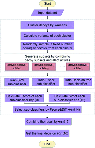
The ENS-VS construction process (step 3 of Fig. 1) includes the following steps (Fig. 2).Firstly, the data set of each target is divided into training set, validation set and test set according to the proportion of 8![[thin space (1/6-em)]](https://www.rsc.org/images/entities/char_2009.gif) :
:![[thin space (1/6-em)]](https://www.rsc.org/images/entities/char_2009.gif) 1
1![[thin space (1/6-em)]](https://www.rsc.org/images/entities/char_2009.gif) :
:![[thin space (1/6-em)]](https://www.rsc.org/images/entities/char_2009.gif) 1. Training set is used for training model, validation set is used for adjusting hyperparameters, and test set is used for testing the performance of the model.
1. Training set is used for training model, validation set is used for adjusting hyperparameters, and test set is used for testing the performance of the model.
Secondly, a number of decoy subsets with the same size as actives are sampled from the original decoys. Each subset of decoys and all of actives compose a subset for training sub-classifier, which contains part information of decoys and all information of actives. We use these subsets to train sub-classifiers separately, and combine the trained sub-classifiers by bagging. Undersampling is an efficient strategy to deal with class imbalance. However, the drawback of undersampling48 is that it throws away many potentially useful data. But our algorithm makes better use of the majority class than undersampling, because multiple subsets contain more information than a single one. In order to select independent identical distribution samples, stratified sampling method is used to perform decoy subset sampling. Decoys are clustered by k-means algorithm, and the number of samples that selected from each cluster is determined by the variance of each cluster (eqn (8)). When the variance of the cluster is high, the data in the cluster are sparse, thus more samples need to be sampled from the cluster to keep the structural feature information of the original dataset. On the contrary, when the variance is low, the data in the cluster are relatively close, thus less samples need to be sampled from the cluster. Let μi (eqn (6)) and σi2 (eqn (7)) represent the mean value and the variance of cluster Ci, respectively. The number of samples should be extracted from one cluster is calculated by eqn (8).
 | (6) |
 | (7) |
 | (8) |

Thirdly, three types of classifiers including SVM,49 decision tree39 and Fisher50 are trained on each training subset. Fscore&Diff method is designed to select a good and different single classifier among all the sub-classifiers. Fscore is calculated by eqn (9) and Diff is calculated by eqn (12). Fscore&Diff method selects a sub-classifier whose Fscore is greater than and Diff is less than the average value of all the sub-classifiers.
| Fscore = (2 × precision × recall)/(precision + recall) | (9) |
| Precision = TP/(TP + FP) | (10) |
| Recall = TP/P | (11) |
 | (12) |
Finally, all generated classifiers are then combined by the weighted average method for the final decision. The weight of each classifier is calculated as follows:
 | (13) |
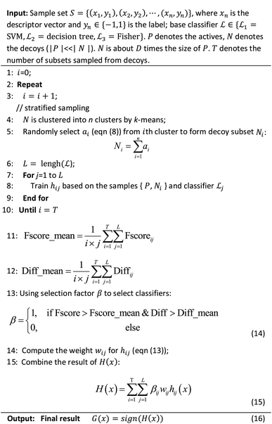
The parameters of sub-classifiers are set as follows: SVM classifier uses linear kernel, and decision tree and Fisher use default parameters. The hyperparameter to be adjusted is the number of the subsets. We use Matlab 2014a software25 to implement this method. The core algorithm of ENS-VS is listed in Table 4.
2.6 Evaluation metrics
Receiver Operating Characteristic curve (ROC), Area Under Curve (AUC), Matthews correlation coefficient (MCC), the enrichment factor (EF) 1% values and the EF 10% values were used to evaluate the performance of this method. The ROC curve is used to visualize the performance of a classifier. AUC represents the probability that a randomly chosen positive sample is ranked higher than a randomly chosen negative sample. MCC is used in machine learning as a measure of the quality of binary (two-class) classifications. It takes into account true positives (TP), false positives (FP), true negatives (TN) and false negatives (FN); and it is generally regarded as a balanced measure which can be used even if the classes are of very different sizes. This value is calculated by eqn (17). EF values are commonly used in machine learning studies as accuracy metrics. The EF x% value is defined as the ratio between the predicted hit rate and the random hit rate, when the top x% ranked compounds are selected as actives. This value is calculated by eqn (18).
 | (17) |
 | (18) |
3. Results and discussion
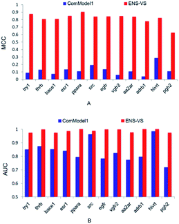
In order to find out the points that contribute to the performance of ENS-VS, we designed three comparison tests based on the 12 datasets in Table 1. The MCC and AUC were used as the metrics for evaluation. The Mann–Whitney U test was used for testing the significance.First, we used protein–ligand interaction descriptor instead of the combination descriptor. This comparison model is denoted as ComModel1. The MCC and AUC results for 12 targets are presented in Fig. 3. The MCC and AUC of ComModel1 were all less than those of ENS-VS for 12 targets. The mean MCC and mean AUC of ComModel1 (MCC = 0.121, AUC = 0.836) were both statistically significantly less than those of ENS-VS (MCC = 0.82, AUC = 0.989), with p < 0.05 (Fig. S1†). It can be seen that the combination descriptor selected by ENS-VS is effective for improving the performance of the VS model.
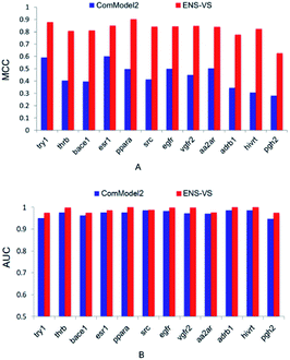
Second, ENS-VS was modified by only undersampling once from decoys. This comparison model is denoted as ComModel2. The results are presented in Fig. 4. The MCC and AUC of ComModel2 were less than those of ENS-VS for each target. The mean MCC and AUC of ENS-VS (MCC = 0.82, AUC = 0.989) were statistically significantly better than those of ComModel2 (MCC = 0.44, AUC = 0.973), with p < 0.05 (Fig. S2†). It is revealed that the processing method for the problem of data imbalance in this study is effective for improving the prediction performance of the VS model.
Third, three types of classifiers in ENS-VS were replaced by only one type of classifier: SVM, decision tree and Fisher, denoted as ComModel3_SVM, ComModel3_Dtree and ComModel3_Fisher, respectively. The mean MCC of ENS-VS was statistically significantly higher than that of ComModel3_SVM, ComModel3_Dtree and ComModel3_Fisher (MCC: ENS-VS = 0.82, ComModel3_SVM = 0.75, ComModel3_Dtree = 0.60, ComModel3_Fisher = 0.60), with P < 0.05 (Fig. 5). The AUC of ENS-VS was statistically significantly higher than that of ComModel3_SVM and ComModel3_Dtree, and had no significant difference compared with ComModel3_Fisher (AUC: ENS-VS = 0.989, ComModel3_SVM = 0.984, ComModel3_Dtree = 0.978 and ComModel3_Fisher = 0.99). The results show that ENS-VS integrating three types of classifier effectively improves the prediction performance of the VS model.
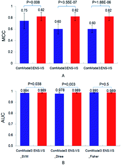 | ||
| Fig. 5 The MCC and AUC of ComModel3_SVM, ComModel3_Dtree, ComModel3_Fisher and ENS-VS for 12 targets. | ||
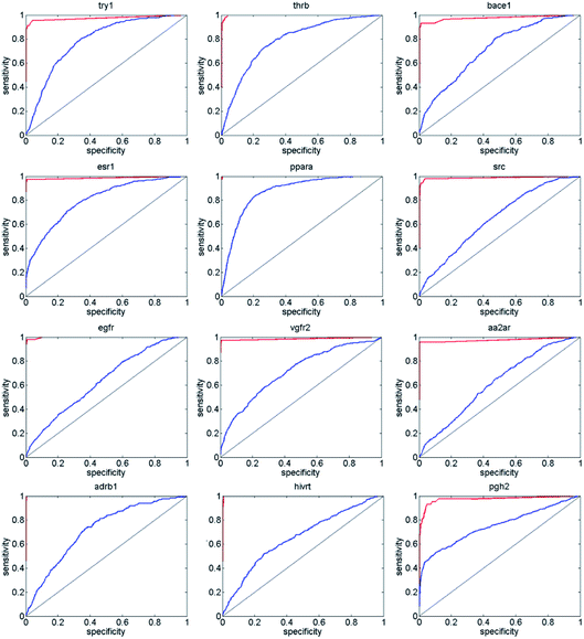
Next, we compared ENS-VS with Autodock vina,11 because we used Vina to generate the poses of the ligands in ENS-VS. The EF and AUC results for the diverse subsets of DUD-E are shown in Table 5. The ROC curves are shown in Fig. 6. The EF 1% and EF 10% results for ENS-VS were both improved significantly for all twelve targets. On average, the EF 1% for ENS-VS was 6 times higher than that for Vina, which indicated that 6 times more active compounds were found by ENS-VS than by Vina on average when the top 1% ranked compounds were biologically assayed for these target proteins. The ROC curve of ENS-VS was very close to the upper left corner for each target, which means that the classifier is effective.
| Target | EF 1% | EF 10% | AUC | |||
|---|---|---|---|---|---|---|
| Vina | ENS-VS | Vina | ENS-VS | Vina | ENS-VS | |
| a The bold means the best value among the two models. | ||||||
| try1 | 12.71 | 58 | 4.59 | 9.78 | 0.786 | 0.974 |
| thrb | 3.9 | 53.7 | 3.75 | 9.99 | 0.798 | 0.998 |
| bace1 | 4.94 | 59.5 | 2.97 | 9.3 | 0.713 | 0.975 |
| esr1 | 18.23 | 53 | 4.49 | 9.73 | 0.801 | 0.986 |
| ppara | 6.7 | 51 | 5.6 | 9.99 | 0.871 | 0.999 |
| src | 3.8 | 55.44 | 2.02 | 9.8 | 0.647 | 0.988 |
| egfr | 3.53 | 65 | 2.04 | 9.81 | 0.634 | 0.998 |
| vgfr2 | 9.06 | 61 | 3.42 | 10 | 0.714 | 0.998 |
| aa2ar | 2.08 | 62.97 | 1.68 | 9.58 | 0.616 | 0.977 |
| adrb1 | 3.23 | 64 | 2.47 | 10 | 0.717 | 0.999 |
| hivrt | 4.46 | 56 | 2.23 | 10.02 | 0.654 | 0.999 |
| pgh2 | 24.44 | 46.09 | 5.1 | 9.32 | 0.75 | 0.974 |
| Average | 8.09 | 57.14 | 3.36 | 9.78 | 0.725 | 0.989 |
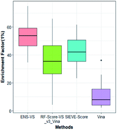
We also considered a comparison with RF-Score-VS_v3_vina22 and SIEVE-Score.51 RF-Score-VS20–22 is a state-of-the-art machine learning-based scoring function. RF-Score-VS_v3_vina is the latest version of RF-Score-VS with docking pose generation by Vina. SIEVE-Score is the newest study about virtual screening method and it has been proved that SIEVE-Score achieves a better performance than three versions of RF-Score-VS. Fig. 7 shows boxplots for ENS-VS, Autodock vina, RF-Score-VS_v3_vina and SIEVE-Score on 37 targets. The results of RF-Score-VS and SIEVE-Score are taken from the original paper of SIEVE-Score.51 Each boxplot shows the EF 1% results on the DUD-E datasets. The EF 1% of RF-Score-VS_v3_vina was higher than that of Vina and less than that of SIEVE-Score. But the performance of ENS-VS about EF 1% was the best among the four methods. Fig. 8 presents a scatter plot of the EF 1% results for ENS-VS vs. SIEVE-Score. Each point represents a target. ENS-VS achieved better predictions for 30 of the 37 DUD-E targets and was tied with SIEVE-Score for the remaining seven targets. The overall EF 1% of ENS-VS for all 37 targets was significantly higher than that of SIEVE-Score (mean EF 1%: ENS-VS = 52.77, SIEVE-Score = 42.64), with p < 0.05. Similarly, the overall EF 10% (mean EF 10%: ENS-VS = 9.72, SIEVE-Score = 7.66) and AUC (mean AUC: ENS-VS = 0.982, SIEVE-Score = 0.912) were also significantly higher (Fig. S3†).
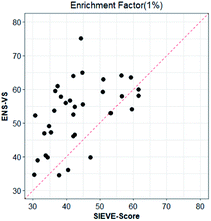 | ||
| Fig. 8 Scatter plot of the EF 1% results of ENS-VS and SIEVE-Score. Each point corresponds to the results for one target protein in the DUD-E dataset. The dotted line represents identical results. | ||
We further compared our method with the recent similar research. The selected methods are shown as follows:
Refmodel1: Yan et al.13 developed a classification model (PLEIC-SVM) with protein–ligand empirical interaction components as descriptors.
Refmodel2: Ragoza et al.16 proposed a neural network for protein–ligand scoring consisting of three convolutional layers. They scored all docked poses using a single, universal model, and took the maximum as the final score.
Refmodel3: Fergus et al.34 coupled densely connected CNN with a transfer learning approach to produce an ensemble of protein family-specific models.
Refmodel4: Janaina et al.33 proposed a deep learning approach to improve docking-based virtual screening, which outperformed the other 25 docking methods in both AUC ROC and enrichment factor when evaluated on the DUD datasets.
Excluding try1 data set, the AUC value of ENS-VS is the highest of the five methods for the other eleven targets, and the standard deviation of ENS-VS is the lowest (Table 6), which suggests that the performance of ENS-VS is better than the other four methods, and ENS-VS has strong robustness.
| Targets | Refmolde1 | Refmolde2 | Refmolde3 | Refmolde4 | ENS-VS |
|---|---|---|---|---|---|
| a The bold means the best value among the five models. | |||||
| try1 | 0.95 | 0.953 | 0.996 | — | 0.974 |
| thrb | 0.95 | 0.924 | 0.978 | — | 0.998 |
| bace1 | 0.91 | 0.808 | 0.930 | — | 0.975 |
| esr1 | 0.97 | 0.930 | 0.951 | — | 0.986 |
| ppara | 0.92 | 0.874 | 0.988 | 0.90 | 0.999 |
| src | 0.93 | 0.950 | 0.986 | 0.85 | 0.988 |
| egfr | 0.93 | 0.966 | 0.985 | 0.86 | 0.998 |
| vgfr2 | 0.95 | 0.967 | 0.993 | 0.90 | 0.998 |
| aa2ar | 0.95 | 0.941 | 0.908 | 0.77 | 0.977 |
| adrb1 | 0.95 | 0.876 | 0.947 | — | 0.999 |
| hivrt | 0.89 | 0.734 | 0.768 | 0.88 | 0.999 |
| pgh2 | 0.90 | 0.840 | 0.877 | — | 0.974 |
| Average | 0.933 | 0.897 | 0.942 | 0.737 | 0.989 |
| SD | 0.024 | 0.073 | 0.066 | 0.049 | 0.011 |
We also used DEKOIS 2.0 database as independent test sets and performed the test by Vina, Glide, SIEVE-Score, RF-Score-VS_v3_vina and ENS-VS, respectively. The methodology is described in more detail in the Methods section. The EF 1%, EF 10% and AUC of Vina, Glide, SIEVE-Score, RF-Score-VS_v3_vina and ENS-VS are shown in Table 7. Except adrb2 and the EF 10% of fa10, ENS-VS outperformed the other four methods for all the metrics. The mean EF 1%, EF 10% and AUC of ENS-VS are the best among the five methods. Therefore, ENS-VS performs better than Vina, Glide, SIEVE-Score and RF-Score-VS_v3_vina for DEKOIS test sets. The mean EF 1%, EF 10% and AUC of ENS-VS for DEKOIS test sets are all less than those for DUD-E test sets. The reason may be in part that the ligand structural similarity between the training set and the test set of DUD-E is higher than that between the test set of DEKOIS and the training set of DUD-E.
| Target | EF 1% | EF 10% | AUC | ||||||||||||
|---|---|---|---|---|---|---|---|---|---|---|---|---|---|---|---|
| Vina | Glide | SIEVE-Score | RF-Score-VS_v3_vina | ENS-VS | Vina | Glide | SIEVE-Score | RF-Score-VS_v3_vina | ENS-VS | Vina | Glide | SIEVE-Score | RF-Score-VS_v3_vina | ENS-VS | |
| a The bold means the best value among the five methods. | |||||||||||||||
| aa2ar | 0 | 7.8 | 34.7 | 16.5 | 42.9 | 1.2 | 1.4 | 8.7 | 5.6 | 9.0 | 0.744 | 0.758 | 0.824 | 0.805 | 0.895 |
| aces | 8.6 | 16.9 | 30.1 | 24.6 | 33.4 | 3.4 | 7.0 | 6.5 | 5.8 | 8.5 | 0.721 | 0.81 | 0.805 | 0.758 | 0.827 |
| adrb2 | 4.8 | 6.7 | 32.6 | 17.9 | 28.7 | 2.7 | 2.8 | 9.8 | 4.7 | 8.0 | 0.698 | 0.715 | 0.819 | 0.724 | 0.798 |
| akt1 | 7.5 | 13.6 | 27.4 | 22.5 | 30.4 | 3.8 | 1.5 | 5.0 | 4.8 | 6.7 | 0.675 | 0.644 | 0.753 | 0.712 | 0.802 |
| fa10 | 5.3 | 16.5 | 28.8 | 16.8 | 35.7 | 2.2 | 5.8 | 6.4 | 3.5 | 6.0 | 0.758 | 0.792 | 0.842 | 0.776 | 0.855 |
| egfr | 0 | 11.2 | 12.6 | 10.8 | 18.8 | 1.6 | 4.0 | 3.5 | 2.1 | 5.8 | 0.642 | 0.704 | 0.696 | 0.677 | 0.724 |
| hivrt | 0 | 7.5 | 17.5 | 11.3 | 22.3 | 1.8 | 1.5 | 6.8 | 2.8 | 8.3 | 0.607 | 0.592 | 0.652 | 0.628 | 0.695 |
| ppara | 0 | 5.7 | 20.8 | 9.7 | 25.6 | 2.0 | 3.2 | 7.3 | 3.9 | 8.0 | 0.690 | 0.698 | 0.727 | 0.701 | 0.746 |
| Average | 3.28 | 10.7 | 25.56 | 16.27 | 29.73 | 2.34 | 3.4 | 6.75 | 4.15 | 7.54 | 0.692 | 0.714 | 0.765 | 0.723 | 0.793 |
ENS-VS succeeds in improving the virtual screening accuracy. There are several reasons. First, the combination descriptor can effectively describe both the characteristic of protein–ligand interactions and the structural characteristic of ligands. After PCA dimension reduction, the number of descriptor was moderate. Thus the combination descriptor is able to not only improve the performance of the model but also prevent overfitting. Second, in order to solve the severe imbalance issue of the dataset that was often ignored in previous studies, we designed a method using the ensemble learning mechanism to sample the decoys. Several subsets of decoys with the same size as actives were sampled from original decoys by stratified sampling. The subset of decoys and all of actives composed a subset for training sub-classifier. The final result was decided by all the sub-classifiers. In this way, the decoys are under-sampled in each sub-classifier, but the important information of the decoys is not lost in the whole situation. Third, to solve the problem that a single machine learning method is not suitable for most targets, ENS-VS integrates a variety of classifiers, i.e. SVM, decision tree and Fisher, to increase diversity, and adaptively selects suitable classifiers for different targets by Fscore&Diff method. It can improve the performance and enhance the robustness of the model for different targets by combining the advantages of three types of classifiers.
Therefore, from the above analysis, we can conclude that the performance improvement of ENS-VS is related to the selection of descriptors, imbalanced data processing measure and ensemble learning method.
Autodock vina is a generic scoring function, which has the advantage of being applicable to any target without retraining. But it is not the case of the better performing target-specific scoring functions. The hit rate is low when Vina is used for virtual screening.52,53 But using ENS-VS after the pose generation by Vina can improve the accuracy of virtual screening significantly. Another advantage of ENS-VS is that it can be used in combination with other docking software besides Autodock vina to improve their performance of virtual screening.
However, this method is based on ensemble learning, it will increase the running time. Therefore, in the future, we will research on the parallel implementation of ENS-VS to improve the execution speed.
4. Conclusion
In this study, we developed a target-specific virtual screening method called ENS-VS to improve the accuracy of structure-based virtual screening. The combination descriptor of protein–ligand interaction energy term and ligand structure vector representation is used; the processing measure for data imbalanced problem is designed and SVM, decision tree and Fisher classifier are integrated in ENS-VS. We performed comprehensive comparisons of this method with several state-of-the-art methods, namely, Autodock vina, Glide, RF-Score-VS and SIEVE-Score, etc. ENS-VS achieved a significant improvement in screening accuracy for different target proteins in the DUD-E and DEKOIS 2.0 benchmark database based on the EF 1%, EF 10% and the AUCs of the ROC curves. Moreover, ENS-VS can be used in combination with any docking software to improve their performance of virtual screening.Conflicts of interest
There are no conflicts to declare.Acknowledgements
This work was supported by Science and Technology Poverty Alleviation Project of Liangshan (No. 18YYJS0041), Science and Technology Program of Luzhou (No. 20/00022585), and the Introducing Talent Start-up Foundation of Southwest Medical University (No. 40/00040142).References
- C. F. Perkinson, D. P. Tabor, M. Einzinger, D. Sheberla, H. Utzat, T.-A. Lin, D. N. Congreve, M. G. Bawendi, A. Aspuru-Guzik and M. A. Baldo, J. Chem. Phys., 2019, 151, 121102 CrossRef.
- A. R. Rosales, J. Wahlers, E. Limé, R. E. Meadows, K. W. Leslie, R. Savin, F. Bell, E. Hansen, P. Helquist and R. H. Munday, Nat. Catal., 2019, 2, 41 CrossRef CAS.
- G. Eren, A. Bruno, S. Guntekin-Ergun, R. Cetin-Atalay, F. Ozgencil, Y. Ozkan, M. Gozelle, S. G. Kaya and G. Costantino, J. Mol. Graphics Modell., 2019, 89, 60–73 CrossRef CAS PubMed.
- K. L. Damm-Ganamet, N. Arora, S. Becart, J. P. Edwards, A. D. Lebsack, H. M. McAllister, M. I. Nelen, N. L. Rao, L. Westover and J. J. Wiener, J. Chem. Inf. Model., 2019, 59, 2046–2062 CrossRef CAS PubMed.
- L. Mazalan, A. Bell, L. Sbaffi and P. Willett, ChemMedChem, 2018, 13, 582–587 CrossRef CAS PubMed.
- J. P. Arcon, L. A. Defelipe, E. D. Lopez, O. Burastero, C. P. Modenutti, X. Barril, M. A. Marti and A. G. Turjanski, J. Chem. Inf. Model., 2019, 59, 3572–3583 CrossRef CAS.
- J. Vucicevic, K. Nikolic and J. B. Mitchell, Curr. Med. Chem., 2019, 26, 3874–3889 CrossRef CAS PubMed.
- R. A. Friesner, R. B. Murphy, M. P. Repasky, L. L. Frye, J. R. Greenwood, T. A. Halgren, P. C. Sanschagrin and D. T. Mainz, J. Med. Chem., 2006, 49, 6177 CrossRef CAS PubMed.
- G. Jones, P. Willett and R. C. Glen, et al., J. Mol. Biol., 1997, 267, 727–748 CrossRef CAS.
- G. M. Morris, D. S. Goodsell and R. S. Halliday, et al., J. Comput. Chem., 1998, 19, 1639–1662 CrossRef CAS.
- O. Trott and A. J. Olson, J. Comput. Chem., 2010, 31, 455–461 CAS.
- P. Harrington, Machine Learning in Action, Manning Publications Co, 2012 Search PubMed.
- Y. Yan, W. Wang, Z. Sun, J. Z. Zhang and C. Ji, J. Chem. Inf. Model., 2017, 57, 1793–1806 CrossRef CAS PubMed.
- S. L. Kinnings, N. Liu, P. J. Tonge, R. M. Jackson, L. Xie and P. E. Bourne, J. Chem. Inf. Model., 2011, 51, 408–419 CrossRef CAS PubMed.
- J. C. Pereira, E. R. Caffarena and C. N. Dos Santos, J. Chem. Inf. Model., 2016, 56, 2495–2506 CrossRef CAS.
- M. Ragoza, J. Hochuli, E. Idrobo, J. Sunseri and D. R. Koes, J. Chem. Inf. Model., 2017, 57, 942–957 CrossRef CAS PubMed.
- P. J. Ballester and J. B. Mitchell, Bioinformatics, 2010, 26, 1169–1175 CrossRef CAS PubMed.
- H. M. Ashtawy and N. R. Mahapatra, BMC Bioinf., 2015, 16, S8 CrossRef PubMed.
- H. M. Ashtawy and N. R. Mahapatra, J. Chem. Inf. Model., 2017, 58, 119–133 CrossRef PubMed.
- P. J. Ballester and J. B. Mitchell, Bioinformatics, 2010, 26, 1169–1175 CrossRef CAS PubMed.
- P. J. Ballester, A. Schreyer and T. L. Blundell, J. Chem. Inf. Model., 2014, 54, 944–955 CrossRef CAS PubMed.
- H. Li, K. S. Leung, M. H. Wong and P. J. Ballester, Mol. Inf., 2015, 34, 115–126 CrossRef CAS PubMed.
- W. T. Mooij and M. L. Verdonk, Proteins: Struct., Funct., Bioinf., 2005, 61, 272–287 CrossRef CAS PubMed.
- D. Wang, X. Ding, C. Cui, Z. Xiong, M. Zheng, X. Luo, H. Jiang and K. Chen, Front. Pharmacol., 2019, 10, 924 CrossRef PubMed.
- C. Springer, H. Adalsteinsson, M. M. Young, P. W. Kegelmeyer and D. C. Roe, J. Med. Chem., 2005, 48, 6821–6831 CrossRef CAS PubMed.
- C. Da and D. Kireev, J. Chem. Inf. Model., 2014, 54, 2555–2561 CrossRef CAS PubMed.
- Z. Deng, C. Chuaqui and J. Singh, J. Med. Chem., 2004, 47, 337–344 CrossRef CAS PubMed.
- T. Sato, T. Honma and S. Yokoyama, J. Chem. Inf. Model., 2009, 50, 170–185 CrossRef PubMed.
- M. M. Mysinger, M. Carchia, J. J. Irwin and B. K. Shoichet, J. Med. Chem., 2012, 55, 6582–6594 CrossRef CAS PubMed.
- N. Huang, B. K. Shoichet and J. J. Irwin, J. Med. Chem., 2006, 49, 6789–6801 CrossRef CAS PubMed.
- S. L. Kinnings, N. Liu, P. J. Tonge, R. M. Jackson, L. Xie and P. E. Bourne, J. Chem. Inf. Model., 2011, 51, 408–419 CrossRef CAS PubMed.
- V. B. Sulimov, I. V. Gribkova, M. P. Kochugaeva, E. V. Katkova, A. V. Sulimov, D. C. Kutov, K. S. Shikhaliev, S. M. Medvedeva, M. Y. Krysin and E. I. Sinauridze, BioMed Res. Int., 2015, 2015, 1–15 CrossRef PubMed.
- J. C. Pereira, E. R. Caffarena and C. N. dos Santos, J. Chem. Inf. Model., 2016, 56, 2495–2506 CrossRef CAS PubMed.
- F. Imrie, A. R. Bradley, M. van der Schaar and C. M. Deane, J. Chem. Inf. Model., 2018, 58, 2319–2330 CrossRef CAS PubMed.
- C. J. Burges, Simplified support vector decision rules, in ICML, 1996, pp. 71–77 Search PubMed.
- M. T. Hagan, M. Beale and M. Beale, Neural network design, 2002 Search PubMed.
- P. Lim, C. K. Goh and K. C. Tan, IEEE Trans. Cybern., 2016, 47, 2850–2861 Search PubMed.
- T.-Y. Liu, Easyensemble and feature selection for imbalance data sets, in IJCBS, 2009, pp. 517–520 Search PubMed.
- J. R. Quinlan, Mach. Learn., 1986, 1, 81–106 Search PubMed.
- D. Díaz-Vico and J. R. Dorronsoro, IEEE Trans. Neural Netw. Learn. Syst., 2019, 99–111 Search PubMed.
- M. R. Bauer, T. M. Ibrahim, S. M. Vogel and F. M. Boeckler, J. Chem. Inf. Model., 2013, 53, 1447–1462 CrossRef CAS PubMed.
- G. M. Morris, R. Huey, W. Lindstrom, M. F. Sanner, R. K. Belew, D. S. Goodsell and A. J. Olson, J. Comput. Chem., 2009, 30, 2785–2791 CrossRef CAS PubMed.
- O. Trott and A. J. Olson, J. Comput. Chem., 2010, 31, 455–461 CAS.
- F. Boyles, C. M. Deane and G. M. Morris, Bioinformatics, 2020, 36, 758–764 Search PubMed.
- A. D. Hill and P. J. Reilly, Methods Mol. Biol., 2015, 1273, 467 CrossRef CAS PubMed.
- S. Jaeger, S. Fulle and S. Turk, J. Chem. Inf. Model., 2018, 58, 27–35 CrossRef CAS PubMed.
- S. Mika, B. Schölkopf, A. J. Smola, K.-R. Müller, M. Scholz and G. Rätsch, Kernel PCA and de-noising in feature spaces, in Adv. Neural Inf. Process Syst., 1999, pp. 536–542 Search PubMed.
- C. Drummond and R. C. Holte, Workshop learning from imbalanced data sets II, in Proc. Int. Conf. Machine Learning, 2003 Search PubMed.
- A. Al-Anazi and I. Gates, Eng. Geol., 2010, 114, 267–277 CrossRef.
- P. N. Belhumeur, J. P. Hespanha and D. J. Kriegman, IEEE Trans. Pattern Anal. Mach. Intell., 1997, 711–720 CrossRef.
- N. Yasuo and M. Sekijima, J. Chem. Inf. Model., 2019, 59, 1050–1061 CrossRef CAS.
- M. Su, Q. Yang, Y. Du, G. Feng, Z. Liu, Y. Li and R. Wang, J. Chem. Inf. Model., 2018, 59, 895–913 CrossRef PubMed.
- J. Li, A. Fu and L. Zhang, Interdiscip. Sci.: Comput. Life Sci., 2019, 1–9 Search PubMed.
Footnote |
| † Electronic supplementary information (ESI) available: Supplemental file 1 (Fig. S1–S3). See DOI: 10.1039/c9ra09211k |
| This journal is © The Royal Society of Chemistry 2020 |

