DOI:
10.1039/D0NA00167H
(Paper)
Nanoscale Adv., 2020,
2, 2540-2547
Rapidly and accurately shaping the intensity and phase of light for optical nano-manipulation†
Received
28th February 2020
, Accepted 28th April 2020
First published on 29th April 2020
Abstract
Holographic optical tweezers can be applied to manipulate microscopic particles in various optical patterns, which classical optical tweezers cannot do. This ability relies on accurate computer-generated holography (CGH), yet most CGH techniques can only shape the intensity profiles while the phase distributions remain poor. Here, we introduce a new method for fast generation of holograms that allows for accurately shaping both the intensity and phase distributions of light. The method uses a discrete inverse Fourier transform formula to directly calculate a hologram in one step, in which a random phase factor is introduced into the formula to enable complete control of intensity and phase. Various optical patterns can be created, as demonstrated by the experimentally measured intensity and phase profiles projected from the holograms. The high-quality shaping of intensity and phase of light provides new opportunities for optical trapping and manipulation, such as controllable transportation of nanoparticles in optical trap networks with variable phase profiles.
1. Introduction
Since Arthur Ashkin invented the classical optical tweezers (i.e., a tightly focused laser beam),1 various optical trapping systems have been developed.2,3 Among them, holographic optical tweezers have attracted much attention due to their several advantages, including dynamic control, high diffraction efficiency, and great flexibility.2–4 Holographic optical tweezers provide versatile routes for trapping, sorting, transporting, and assembling of micron and nanoparticles.2,5 In addition, as a general optical and electronic technology, optical holography has been a rapidly growing field in the past two decades. It has found a wide range of applications in laser beam shaping, optical communication, 3D display, biological imaging, microfluidics, atom cooling, and quantum manipulation.6–16
A phase-only spatial light modulator (SLM), which can be easily used to generate a desired light field with CGH, has been one of the most attractive devices for building holographic optical tweezers.17,18 A phase-only SLM consists of a 2D matrix of liquid crystal cells individually controlled by electronic signals. It can retard the optical phase from 0 to 2π, which is determined by the corresponding gray level of the calculated CGH. In the past several years, various methods have been proposed for the design of phase-only holograms, which generally can be categorized as the iterative algorithms, non-iterative algorithms, and integral methods. For most iterative algorithms, such as the iterative Fourier transform algorithm,19 direct binary search,20 Gerchburg–Saxton algorithm,21–24 and adaptive-additive algorithm,25 the intensity distribution with relatively good uniformity at the output plane can be obtained by iterative searching and optimization. However, the phase distribution is generally poor, which is obviously unfavorable for nanoparticle manipulation when using optical forces arising from phase gradients.26 In addition, the quality of CGH highly depends on the steps and searching algorithm in the optimization process, which largely affects the computation time of hologram generation.
For non-iterative algorithms, the computation time can be reduced, and the speckle noise can be decreased to some extent.27,28 However, the quality of the generated hologram still needs to be improved. In order to achieve simultaneous intensity and phase control, Jesacher et al. proposed a method of using two cascaded phase diffractive elements to separately modulate the amplitude and phase of a laser beam,29 but it is difficult to precisely control the alignment between two phase elements, which easily results in poor quality of the optical field and low efficiency. Later, Bolduc et al. established a similar method of encoding the amplitude and phase of the optical field by using two SLMs, which can be applied in the quantum encryption.30 Besides, Shanblatt et al. presented a method of directly using analytical formula to generate holograms in ring traps with different orientations, which have advantages such as high accuracy and low computation cost.31 Recently, Rodrigo et al. demonstrated a strategy for CGH design of optical traps by using the integral method, which can effectively achieve simultaneous control of intensity and phase distributions.32–37 However, this method is limited to the realization of smooth optical patterns consisting of special curves, termed as superformula curves. If an optical pattern cannot be expressed by a well-defined formula, the integral method cannot be used directly, and some approximations must be made. Particularly, the method is not suitable for designing even ordinary optical profiles, such as straight lines and point arrays. Therefore, it is highly desirable to generate optical fields with complete control of intensity and phase, especially for optical manipulation of nanoparticles.
In this work, we introduce a new approach for generating phase-only holograms that can produce high-quality intensity and phase profiles at the output plane. The approach is a direct computation method for CGH. Its simple calculation leads to low computational cost yet high accuracy. Through numerical simulation and experimental investigation, we show that the intensity and phase distribution can be simultaneously obtained, which is very useful for exploring new functions in optical nano-manipulation.
2. Method
We assume a reflective phase-only SLM is illuminated by a linearly polarized laser beam with a wavelength of λ. The phase-modulated beam is at the back focal plane of a lens with a focus length of f, generating a holographic optical pattern at its front focal plane. The relationship between optical fields at the input and output planes can be written as,38| | 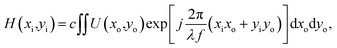 | (1) |
where c is a constant, j is complex unit, H(xi,yi) is the optical field reflected at the input plane, and U(xo,yo) is the desired optical field at the output plane. These optical fields are expressed as,| | U(xo,yo) = au(xo,yo)![[thin space (1/6-em)]](https://www.rsc.org/images/entities/char_2009.gif) exp[jφu(xo,yo)], exp[jφu(xo,yo)], | (2) |
| | | H(xi,yi) = ah(xi,yi)exp[jφh(xi,yi)], | (3) |
Obviously, there exists an inverse Fourier transform relationship between H(xi,yi) and U(xo,yo), as shown in eqn (1). Theoretically, H(xi,yi) can be easily obtained by using a fast inverse Fourier transform (IFFT) if the SLM can modulate both the amplitude and phase. However, commercial SLMs are either amplitude-only or phase-only devices. For example, if the calculated optical field H(xi,yi) is projected on a phase-only SLM, all amplitude information of ah(xi,yi) will be lost, leading to a large discrepancy between the generated optical field U′(xo,yo) and the desired optical field U(xo,yo). Usually, the discrepancy will further increase as the uniformity of ah(xi,yi) gets worse.
From a different standpoint, the optical field H(xi,yi) can be viewed as the superposition of individual plane waves with a weight factor, U(xo,yo). Hence, the eqn (1) can be given using discrete expression,
| |  | (4) |
where Δ
xo and Δ
yo are the single pixel size in the
x and
y direction at the output plane; Δ
xi and Δ
yi are the single pixel size in the
x and
y direction at the input plane;
c′ =
cΔ
xoΔ
yo;
k ∈ [−
K/2,
K/2],
s ∈ [−
S/2,
S/2],
m ∈ [−
M/2,
M/2],
n ∈ [−
N/2,
N/2], in which
K and
S stand for the maximum number of sampling pixels in the
x and
y axis at the output plane, respectively, and
M,
N denote the maximum number of sampling pixels in the
x and
y axis at the input plane, respectively;
U(
k,
s) stands for
U(
kΔ
xo,
sΔ
yo), and
H(
m,
n) denotes
H(
mΔ
xi,
nΔ
yi). Unfortunately, we cannot directly use
eqn (4) to calculate the CGH, as
eqn (4) is mathematically equivalent to
eqn (1). To address this issue, we innovatively modify
eqn (4) by introducing a random phase factor exp
(
jϕ), in which
ϕ =
dm ×
rand,
dm is the modulation depth with a maximum of 2π, and
rand is a function that creates a random number in the interval (0, 1) in each step of calculation. Hence, the
eqn (4) can be written as the following equation:
| |  | (5) |
In this case, a random phase generated by Matlab library function is directly added into each plane wave used as an eigenfunction in the superposition process; therefore eqn (5) is substantially different from eqn (4). Usually, the superposition among different plane waves at the input plane leads to the degradation of uniformity of ah(xi,yi). The random phase is employed to minimize their interference, and reshape the profiles of amplitude ah(xi,yi), so the uniformity of amplitude ah(xi,yi) can be effectively improved, which upgrades the accuracy of intensity and phase profiles at output plane (see Note 1 in ESI†). Accordingly, the phase profiles of holograms can be obtained by,
| | | P(m,n) = arg[H(m,n)], | (6) |
where symbol arg stands for phase angle of
H(
m,
n).
It is worth noting that the holograms in our proposed method are directly calculated in single step, which are different from the conventional iterative methods. The Gerchburg–Saxton algorithm may also use random phases to preset the initial phase of a hologram in the first step of the search process, but the purpose is only to converge to the solution faster.21 Random superposition algorithm is an iterative algorithm, in which random values uniformly distributed in [0, 2π] are added while calculating the phase of linear superposition of single trap hologram. It is helpful for improving its efficiency and reducing its computation cost, which is preferred when requiring frequent calculation of large dynamical optical spot arrays with low symmetry geometries.39 Additionally, a recent report adopted a similar concept of the random phase factor.40 The report shows that Fresnel holograms can produce large volume, high-density, dynamic 3D images for display at different depths by adding random phases into each desired 3-D image, to decrease crosstalk among these different images at output plane. However, the iterative Fourier transform algorithm has been used for generating a set of kinoforms, and phase profiles of each image at different output positions cannot be fully controlled. In our method, the random phase factor is directly introduced in each plane wave of eqn (5) to largely weaken their interference among different plane waves at input plane. The related results reveal that it is very helpful for generating the desired optical traps with accurate control of intensity and phase profiles, which is highly preferred in the optical manipulation of nanoparticles.
3. Results
Our proposed method is employed to generate CGH at the input plane and reconstruct the image at the output plane to test its validation. Our target patterns include point spot arrays, peanut-shaped spot arrays, straight-lines, and rings. In the simulation process, each simulated area has 1024 × 1272 pixels, and its pixel size is 0.139 μm × 0.139 μm at the output plane, and the target optical pattern is located in the simulated area. Similarly, the phase-only SLM has 1024 × 1272 pixels with a pixel size of 12.5 μm × 12.5 μm. The focus length of the objective lens is 3 mm. The related experimental investigations are carried out to further evaluate the proposed method. These experiments were performed in our optical trapping system,41 which includes a CW tunable Ti:Sapphire laser (Spectra-Physics 3900s) operating at a wavelength of 800 nm and producing a TEM00 Gaussian mode. A phase-only SLM (Hamamatsu X13138) is used to modulate the phase of the calculated hologram. A beam profiler (Edmund Optics) is employed for capturing the optical intensity of the reconstructed image, and a Shack-Hartmann wavefront sensor (Thorlabs WFS20-7AR) is used to measure the phase, which has resolution of 1440 × 1080 pixels and arrays of 47 × 35 active lenslets. In addition, a grating phase is added to the calculated hologram to shift the reconstructed image, which can effectively reduce the negative influence from the zero-order optical diffractive spot of SLM.
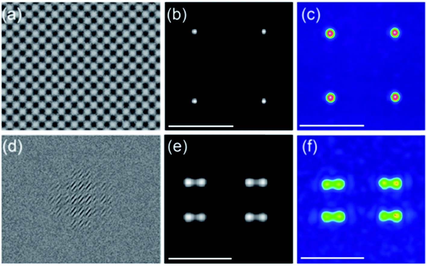
Point spot arrays
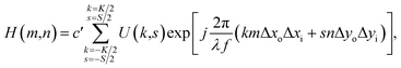
The point spot arrays are conventional optical tweezers, which are widely applied in optical trapping, ranging from atoms to microparticles. Fig. 1(a and b) shows the calculated hologram and reconstructed image of a point optical trap array. The nonuniformity of spot arrays is less than 0.0017. The experimentally measured optical pattern is presented in Fig. 1(c), which agrees well with the reconstructed image and demonstrates that the calculated hologram has high accuracy. The intensity distribution among the optical traps is very identical, which is highly desired for optical trapping. Additionally, the other spot arrays structures including circle spot arrays and 5 × 5 spot arrays are numerically investigated, which reveals that their nonuniformity are also low (see Note 2 in ESI†).
 |
| | Fig. 1 Point and peanut-shaped spot arrays. (a and d) Calculated holograms, (b and e) reconstructed intensity profiles, and (c and f) measured intensity profiles. Note that scale bar is 5 μm. | |
Peanut-shaped spot arrays
The peanut-shaped spot arrays are novel optical traps, which have potential for achieving new functions in optical manipulation.42 Similarly, the computed hologram, reconstructed intensity, and measured intensity are given in Fig. 1(d)–(f), respectively. Again, the intensity distributions among all peanut-shaped spots are nearly identical. In addition, the difference between the simulated results and the experimental results is very small, which further demonstrates that our method can generate high-quality holograms.
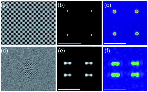
Optical line traps
The optical line traps generated by cylindrical lens holograms have non-uniform intensity and phase distributions,13,15 which limits their application in optical manipulation. Flat-top line traps with specified phase profiles can be produced by a shape-phase modulation approach,43 but the light utilization efficiency is low. Here, we design an optical line pattern, which has uniform optical intensity and phase distribution with a sinusoidal function. The calculated hologram, reconstructed optical intensity, and measured optical intensity are presented in Fig. 2(a)–(c), respectively. Evidently, both the reconstructed optical intensity and measured optical intensity from the hologram have uniform distributions, and the former is consistent with the latter. Particularly, the phase distribution with a sinusoidal function in an optical line trap is realized for the first time. The phase distribution is measured at the output plane of a lens with a focus length of 75 cm.44 In this work, we only measure the phase distribution of the optical line trap due to the limited resolution of the wave-front sensor, which could be inaccurate when measuring the complex wave-fronts of 2D patterns. The designed phase, reconstructed phase, and measured phase of the optical line trap are given in Fig. 2(d)–(f), respectively. The measured phase distribution is in good agreement with the designed and reconstructed phase distributions. The results demonstrate that our method is very helpful for realizing new functions in optical manipulation of nanoparticles by designing different phase distributions.
 |
| | Fig. 2 Optical line trap. (a) Calculated hologram, (b) reconstructed intensity, (c) measured intensity, (d) designed phase, (e) reconstructed phase, and (f) measured phase. Note that the phase profiles are measured by using wavefront sensor at the Fourier plane of SLM, in which lens with focal length of 75 cm is used, and its size is enlarged by about 90 times, and scale bar is 10 μm. | |
2D and 3D optical patterns
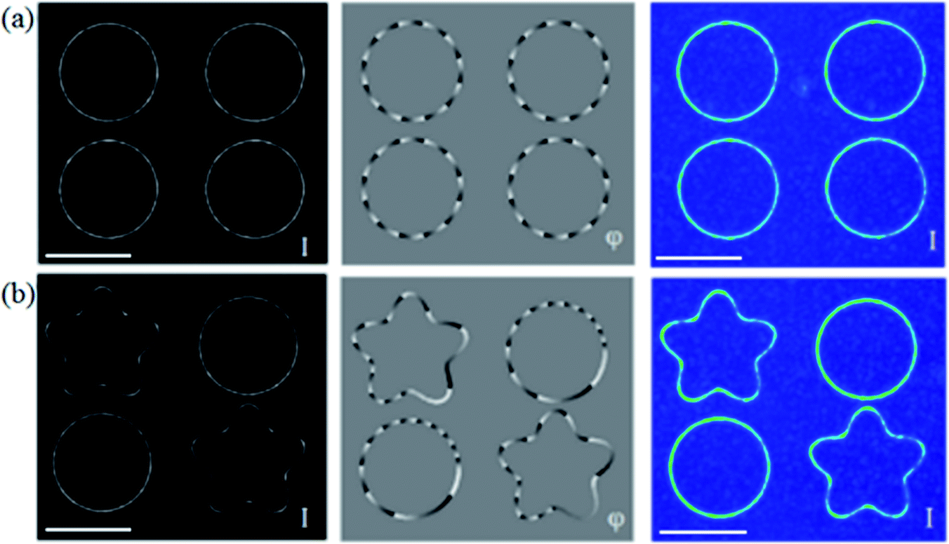
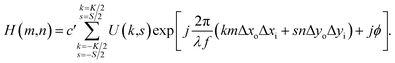
The optical trap arrays with closed curves have attracted increasing attention in recent years.45 For our proposed method, more interestingly, the optical trap arrays can be easily realized by utilizing the convolution theorem from Fourier optics.38 For simplicity, we present two types of optical traps. The first pattern is four identical rings, whose phase profiles are linear. The reconstructed intensity, reconstructed phase, and measured intensity are presented, as shown in the left, middle, and right subfigures of Fig. 3(a), respectively. The second pattern includes two identical rings and two identical stars, whose phase profiles are nonlinear. Similarly, its reconstructed intensity, phase and measured intensity are shown in the left, middle, and right subfigures of Fig. 3(b), respectively. Obviously, the difference between reconstructed and measured intensity in each pattern is very small, which indicates that different array patterns can be easily achieved by using our proposed method. More importantly, the desired phase distribution would not be affected by the desired intensity distribution in our method, which is highly preferred in optical manipulation of particles using phase gradient force. Therefore, arbitrary phase distribution can be accurately achieved by using our method. For the iterative algorithms, however, it remains very difficult to precisely generate the desired phase gradient distribution.
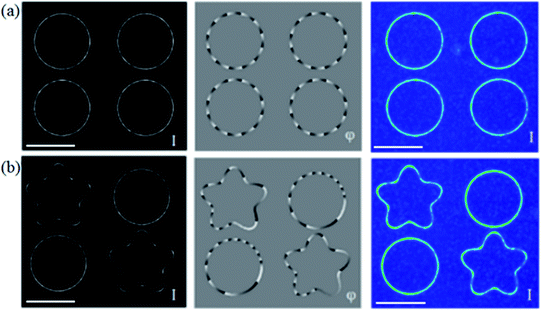 |
| | Fig. 3 Optical trap array of rings and stars. (a and b) Reconstructed intensity (I), reconstructed phase (φ), and measured intensity of ring trap arrays and mixed ring and star traps. Note that in the middle panel of (b), the phase profiles of the rings and stars are nonlinear, and scale bar is 10 μm. | |
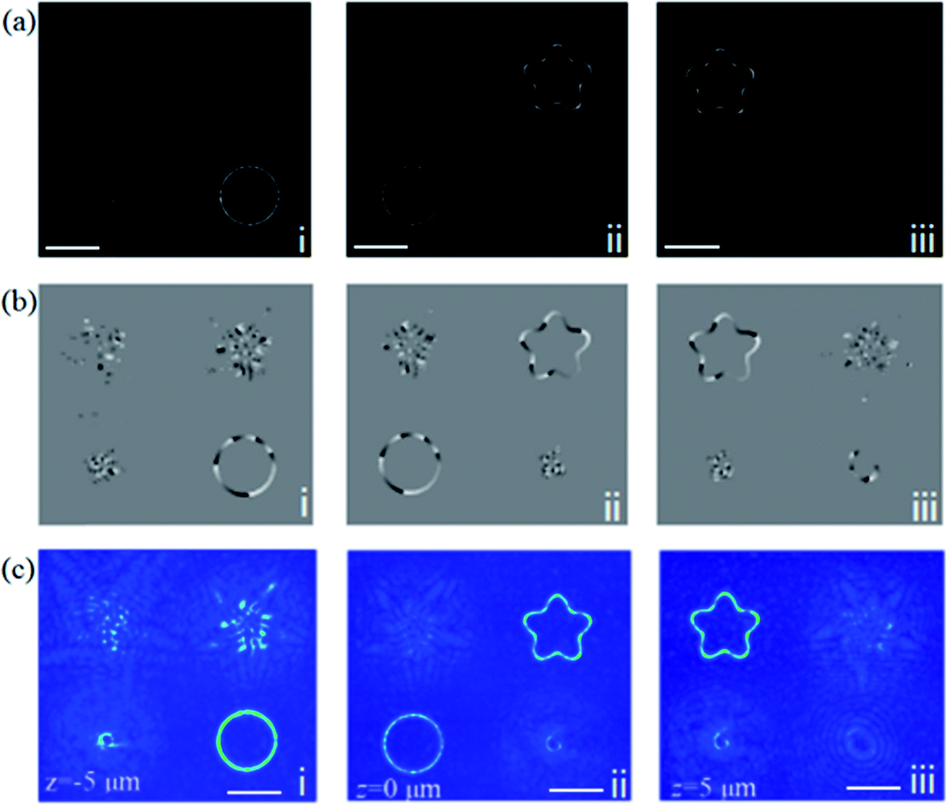
Particularly, 3D optical traps with various closed curves at different regions along light propagation direction can also be easily realized by using our method. The position of each trap can be conveniently controlled by adding a spherical wave phase with πz(xo2 + yo2)/(λf2) in the desired hologram, according to on-demand shifting distance z along optical axis direction. The reconstructed intensity distributions, reconstructed phase profiles and measured intensity distributions at different positions are shown in Fig. 4. The ring and star traps are focused on the focal plane (z = 0), as presented in Fig. 4(b), while the other ring and star traps are axially shifted to the plane of z = −5 μm and z = 5 μm, as shown in Fig. 4(a) and (c), respectively. It finds that the measured intensity distributions are highly consistent with the reconstructed ones. These multiple traps at different axial positions have important applications for simultaneously implementing multitask optical manipulation. Particularly, it needs to note that variation range of grayscale in reconstructed phase is from 0 to 2π, and reconstructed intensity distribution is normalized, whose grayscale range is from 0 to 1.
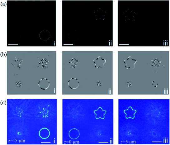 |
| | Fig. 4 3D optical traps at different positions. (a) Reconstructed intensity. (b) Reconstructed phase. (c) Measured intensity. Note that panels i-iii correspond to intensity and phase profiles at position of z = −5 μm, z = 0 μm, and z = 5 μm, respectively. Note that scale bar is 10 μm. | |
Optical manipulation of nanoparticles
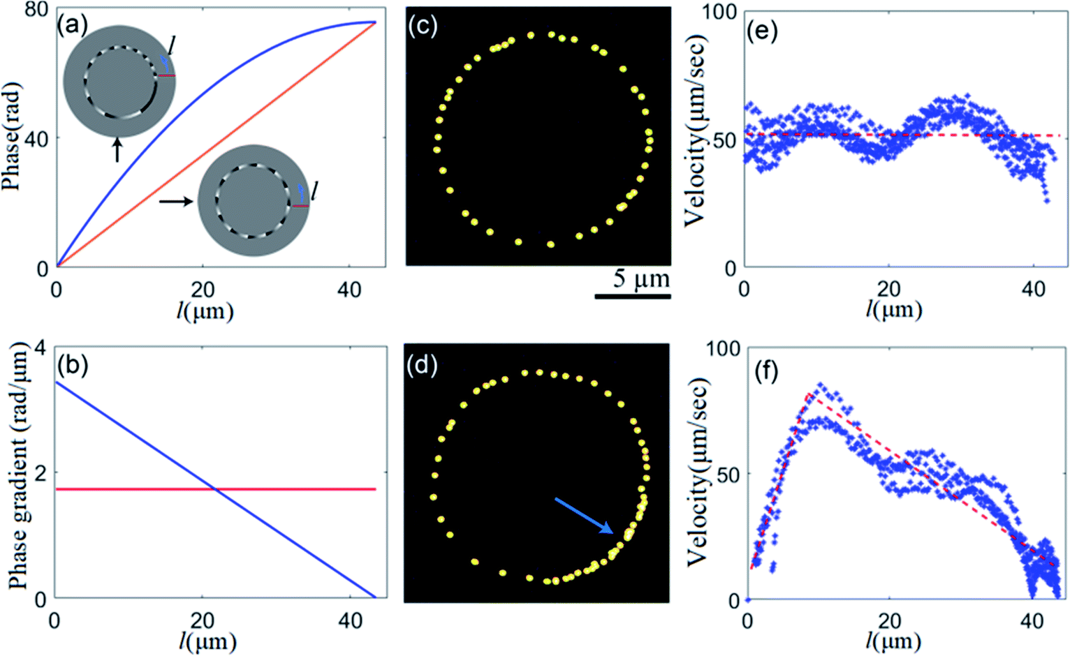
We performed experiments with Au nanoparticles (200 nm in diameter) to evaluate the performance of optical manipulation in ring traps with different phase distributions. The phase distribution and phase gradient along a circle orbit in the counterclockwise direction are presented in Fig. 5(a) and (b), respectively, in which linear and nonlinear phase distributions are denoted by red and blue solid lines, respectively, and the starting points are marked on the reconstructed phase images in the insets of Fig. 5(a). A single Au nanoparticle is driven by the phase gradient force along each circle orbit, as shown in the superimposed dark-field optical images in Fig. 5(c) and (d), and its speed along the circle orbit is closely related to its phase gradient. The small distance between the two adjacent positions indicates lower velocity (e.g., in the portion marked by the arrow in Fig. 5(d), where the phase gradient is small). The measured velocities around the circle orbits are shown in Fig. 5(e) and (f), respectively. For the ring optical trap with linear phase variation, its velocity fluctuates moderately around 51 μm s−1, as marked by a dashed red line in Fig. 5(e). The variation of velocity is due to the anisotropy of optical force in the ring trap created by polarization-dependent focusing of a linearly polarized beam.46 If a radially polarized or azimuthally polarized beam is employed in the ring trap, the anisotropy effect could be largely eliminated. For the ring optical trap with nonlinear phase variation, its velocity rapidly increases in a short distance and then decreases slowly in a long distance. In the beginning, the velocity is very low, but its phase gradient force is large, so its driving force is much larger than its drag force, which leads to rapid increase in velocity. After a short distance, its phase gradient force quickly decreases, so it is smaller than its drag force, causing a decrease in velocity. Its tendency of velocity variation is marked by the dashed red line in Fig. 5(f). Consequently, it reveals that our designed ring trap has high accuracy, which reveals excellent capability of trapping and steering metal nanoparticles in the circle orbit.
 |
| | Fig. 5 Optical manipulation of nanoparticles in ring traps with linear and nonlinear phase profiles. (a) Phase variation along circle orbit, (b) phase gradient along circle orbit, (c) superimpositions of dark-field optical images of the trapped nanoparticles moving in a ring trap for one circle with linear phase variation, (d) superimpositions of dark-field optical images of the trapped nanoparticles moving in a ring trap for one circle with nonlinear phase variation, (e) velocity at different positions of a ring trap with linear phase variation, and (f) velocity at different positions of a ring trap with nonlinear phase variation. Note that the insets in (a) are reconstructed phase images, and in (c and d), the time interval from one position of the nanoparticle to its next position is 20 ms, and optical power is 105 mW. | |
4. Further discussion
Although the generated holograms by our method generally have slight phase noise caused by the introduction of a random phase factor, the reconstructed intensity and phase profiles are not substantially affected by the phase noise (see Note 3 in ESI†). However, a relatively large difference between the obtained pattern and target pattern still exists if its uniformity of amplitude ah(xi,yi) remains poor. To address this issue, pre-compensation can be employed to amend the intensity distribution of the target pattern in advance, which can effectively improve the quality of the obtained pattern (see Note 4 in ESI†). Additionally, it is worth noting that the modulation depth, dm, of the random phase factor should be reasonably chosen. If the modulation depth is too small, the crosstalk between different plane waves at the input plane will not be effectively eliminated. However, if it is too large, the noise in the hologram will have a considerable negative effect on the optical pattern at the output plane. An example of line patterns under different modulation depths is demonstrated (see Note 4 in ESI†). It appears that when the random phase factor is π, its intensity and phase profiles are the most acceptable. Particularly, the comparison of reconstructed intensity and phase profiles generated by different methods, are performed, which further shows that holograms designed by our method can create optical intensity and phase profiles with high quality (see Note 5 in ESI†).
The computation cost is low in our method, which is very helpful for dynamical optical manipulation. As a comparison, we also calculate the hologram of a typical ring trap by using the integral method,33 ant it reveals that the reconstructed intensity and phase are nearly identical to those obtained by our method. Its computation time in integral method is about 90 second, but it is about 13 second in our method.
5. Conclusions
In this work, we have proposed a novel approach for realizing phase-only holograms. The approach is a direct method that uses a discrete inverse Fourier transform formula, in which a random phase factor is introduced. The numerical simulation and experimental work show that high-quality holograms can be achieved using our method. In particular, the desired phase distribution is not affected by the desired intensity distribution, which is useful to accurately obtain a preferred phase distribution. In addition, our optical trapping experiments indicate that the holograms generated by our method are suitable for optical manipulation of nanoparticles. Our approach has several advantages, including simple calculation, low computation cost, high accuracy, and high flexibility for generating different types of optical patterns, which offers great potential in applications including optical trapping, 3D microfabrication, and laser beam shaping.
Conflicts of interest
There are no conflicts to declare.
Acknowledgements
The work is supported by the W. M. Keck Foundation and the Foundation of China Scholarship Council for a visiting scholar fellowship.
References
- A. Ashkin, J. M. Dziedzic, J. E. Bjorkholm and S. Chu, Opt. Lett., 1986, 11, 288–290 CrossRef CAS PubMed.
- M. Woerdemann, C. Alpmann, M. Esseling and C. Denz, Laser Photonics Rev., 2013, 7, 839–854 CrossRef CAS.
- D. Gao, W. Ding, M. Nieto-Vesperinas, X. Ding, M. Rahman, T. Zhang, C. Lim and C. W. Qiu, Light: Sci. Appl., 2017, 6, e17039 CrossRef CAS PubMed.
- D. G. Grier, Nature, 2003, 424, 810–816 CrossRef CAS PubMed.
- A. Jonáš and P. Zemanek, Electrophoresis, 2008, 29, 4813–4851 CrossRef PubMed.
- X. Zhang, J. Jin, M. Pu, X. Li, X. Ma, P. Gao, Z. Zhao, Y. Wang, C. Wang and X. Luo, Nanoscale, 2017, 9, 1409–1415 RSC.
- G.-Y. Lee, G. Yoon, S.-Y. Lee, H. Yun, J. Cho, K. Lee, H. Kim, J. Rho and B. Lee, Nanoscale, 2018, 10, 4237–4245 RSC.
- Y. Zhang, W. Liu, J. Gao and X. Yang, Adv. Opt. Mater., 2018, 6, 1701228 CrossRef.
- S. Jia, J. C. Vaughan and X. Zhuang, Nat. Photonics, 2014, 8, 302–306 CrossRef CAS.
- H. Wang, Y. Liu, Q. Ruan, H. Liu, R. J. H. Ng, Y. S. Tan, H. Wang, Y. Li, C. W. Qiu and J. K. W. Yang, Adv. Opt. Mater., 2019, 7, 1900068 CrossRef.
- I. T. Leite, S. Turtaev, X. Jiang, M. Šiler, A. Cuschieri, P. S. J. Russell and T. Čižmár, Nat. Photonics, 2018, 12, 33–39 CrossRef CAS.
- L. Wang, W. Zhang, H. Yin and X. Zhang, Adv. Opt. Mater., 2019, 7, 1900263 CrossRef.
- F. Nan and Z. Yan, Nano Lett., 2018, 18, 7400–7406 CrossRef CAS PubMed.
- M. Padgett and R. Di Leonardo, Lab Chip, 2011, 11, 1196–1205 RSC.
- F. Nan and Z. Yan, Nano Lett., 2018, 18, 4500–4505 CrossRef CAS PubMed.
- D. Barredo, V. Lienhard, S. de Léséleuc, T. Lahaye and A. Browaeys, Nature, 2018, 561, 79–82 CrossRef CAS.
- Z. Yan, J. E. Jureller, J. Sweet, M. J. Guffey, M. Pelton and N. F. Scherer, Nano Lett., 2012, 12, 5155–5161 CrossRef CAS PubMed.
- O. M. Marago, P. H. Jones, P. G. Gucciardi, G. Volpe and A. C. Ferrari, Nat. Nanotechnol., 2013, 8, 807–819 CrossRef CAS.
- C. Hesseling, M. Woerdemann, A. Hermerschmidt and C. Denz, Opt. Lett., 2011, 36, 3657–3659 CrossRef.
- X. Zhao, J. Li, T. Tao, Q. Long and X. Wu, Opt. Eng., 2012, 51, 015801 CrossRef.
- H. Kim, M. Kim, W. Lee and J. Ahn, Opt. Express, 2019, 27, 2184–2196 CrossRef CAS PubMed.
- S. Tao and W. Yu, Opt. Express, 2015, 23, 1052–1062 CrossRef CAS PubMed.
- Z. Yuan and S. Tao, J. Opt., 2014, 16, 105701 CrossRef.
- L. Wu, S. Cheng and S. Tao, Sci. Rep., 2015, 5, 15426 CrossRef CAS PubMed.
- D. Wang, Y. L. Wu, B. Q. Jin, P. Jia and D. M. Cai, IEEE Photonics J., 2014, 6, 6802111 Search PubMed.
- Y. Roichman, B. Sun, Y. Roichman, J. Amato-Grill and D. G. Grier, Phys. Rev. Lett., 2008, 100, 013602 CrossRef PubMed.
- D. Mengu, E. Ulusoy and H. Urey, Opt. Express, 2016, 24, 4462–4476 CrossRef PubMed.
- H. Pang, J. Wang, M. Zhang, A. Cao, L. Shi and Q. Deng, Opt. Express, 2017, 25, 14323–14333 CrossRef PubMed.
- A. Jesacher, C. Maurer, A. Schwaighofer, S. Bernet and M. Ritsch-Marte, Opt. Express, 2008, 16, 4479–4486 CrossRef PubMed.
- E. Bolduc, N. Bent, E. Santamato, E. Karimi and R. W. Boyd, Opt. Lett., 2013, 38, 3546–3549 CrossRef PubMed.
- E. R. Shanblatt and D. G. Grier, Opt. Express, 2011, 19, 5833–5838 CrossRef CAS PubMed.
- J. A. Rodrigo, M. Angulo and T. Alieva, Opt. Express, 2018, 26, 18608–18620 CrossRef PubMed.
- J. A. Rodrigo and T. Alieva, Optica, 2015, 2, 812–815 CrossRef.
- J. A. Rodrigo and T. Alieva, Sci. Rep., 2016, 6, 33729 CrossRef CAS PubMed.
- J. A. Rodrigo, M. Angulo and T. Alieva, Opt. Lett., 2018, 43, 4244–4247 CrossRef PubMed.
- J. A. Rodrigo, T. Alieva, E. Abramochkin and I. Castro, Opt. Express, 2013, 21, 20544–20555 CrossRef PubMed.
- J. A. Rodrigo and T. Alieva, Sci. Rep., 2016, 6, 35341 CrossRef CAS PubMed.
-
J. W. Goodman, Introduction to Fourier Optics, The McGraw-Hill Companies, Inc., New York, 2005 Search PubMed.
- R. Di Leonardo, F. Ianni and G. Ruocco, Opt. Express, 2007, 15, 1913–1922 CrossRef.
- G. Makey, Ö. Yavuz, D. K. Kesim, A. Turnal, P. Elahi, S. Ilday, O. Tokel and F. Ö. Ilday, Nat. Photonics, 2019, 13, 251–256 CrossRef CAS PubMed.
- F. Han, J. A. Parker, Y. Yifat, C. Peterson, S. K. Gray, N. F. Scherer and Z. Yan, Nat. Commun., 2018, 9, 4897 CrossRef PubMed.
- G. David, K. Esat, I. Thanopulos and R. Signorell, Commun. Chem., 2018, 1, 46 CrossRef.
- Y. Roichman and D. G. Grier, Opt. Lett., 2006, 31, 1675–1677 CrossRef PubMed.
- Z. Yan, M. Sajjan and N. F. Scherer, Phys. Rev. Lett., 2015, 114, 143901 CrossRef PubMed.
- P. Figliozzi, C. W. Peterson, S. A. Rice and N. F. Scherer, ACS Nano, 2018, 12, 5168–5175 CrossRef CAS PubMed.
- P. Figliozzi, N. Sule, Z. Yan, Y. Bao, S. Burov, S. K. Gray, S. A. Rice, S. Vaikuntanathan and N. F. Scherer, Phys. Rev. E, 2017, 95, 022604 CrossRef PubMed.
Footnote |
| † Electronic supplementary information (ESI) available. See DOI: 10.1039/d0na00167h |
|
| This journal is © The Royal Society of Chemistry 2020 |
Click here to see how this site uses Cookies. View our privacy policy here. 
 Open Access Article
 This Open Access Article is licensed under a Creative Commons Attribution-Non Commercial 3.0 Unported Licence
 *ac,
Fan
Nan
b and
Zijie
Yan
*ac,
Fan
Nan
b and
Zijie
Yan