Complex diffusion-based kinetics of photoluminescence in semiconductor nanoplatelets
Received
13th July 2020
, Accepted 2nd October 2020
First published on 19th October 2020
Abstract
We present a diffusion-based simulation and theoretical models for explanation of the photoluminescence (PL) emission intensity in semiconductor nanoplatelets. It is shown that the shape of the PL intensity curves can be reproduced by the interplay of recombination, diffusion and trapping of excitons. The emission intensity at short times is purely exponential and is defined by recombination. At long times, it is governed by the release of excitons from surface traps and is characterized by a power-law tail. We show that the crossover from one limit to another is controlled by diffusion properties. This intermediate region exhibits a rich behaviour depending on the value of diffusivity. The proposed approach reproduces all the features of experimental curves measured for different nanoplatelet systems.
1 Introduction
The hunt for materials and systems with better optical properties has always been one of the focal points of semiconductor research.1 The first classical optoelectronic applications were based mostly on the bulk properties of semiconductors. Recent progress in material synthesis2–4 led to wider research efforts concentrated on low-dimensional structures. In particular, significant attention has been drawn toward the semiconductor nanocrystals, such as quantum dots (QDs) and nanoplatelets (NPLs).5,6 QDs and NPLs show large exciton binding energies7–9 and possess such remarkable properties as narrow emission lines even at room temperature, tunable emission wavelengths, short radiative lifetimes, giant oscillator strengths, high quantum yields and vanishing inhomogeneous broadening.10–14 These properties make them excellent prospective building blocks for future optoelectronic devices such as bright and flexible light emitters,15 or colloidal lasers,8,16 or for biomedical labeling applications.17
Modern techniques of precise colloidal synthesis allow control of the shape,18 size19 and crystal structure of the nanocrystals.20 Among these, there is a growing popularity of colloidal QDs and NPLs of CdSe with atomically defined thickness5,21,22 and various shapes such as pure QDs and NPLs (core) as well as composite core–shell QDs and NPLs or core–crown NPLs. The composites are made of two different semiconductor materials, for instance, CdSe and CdS.
The low-dimensionality of all these structures effects in a decisive way the crystal surface that controls the optical and electronic properties.23 Specifically, the nanocrystal surfaces contain numerous dangling bonds. The dangling bonds that correspond to the undercoordinated surface atoms rearrange themselves by surface reconstruction or adsorb surfactant ligands.24 The latter are utilised during colloidal synthesis as they increase the stability of nanocrystals, prevent crystal stacking and screen them from the environment as well as, most importantly, stabilising the surface by saturating dangling bonds.25 As a result, ligands influence surface trap states and, consequently, control photoluminescence (PL) properties.26,27 Since the PL signal occurs due to electron–hole recombination, the optical properties of colloidal nanocrystals are directly controlled by different kinds of surface traps (reversible and irreversible).
An example of a direct experimental manifestation of the surface trap role in PL signals is the phenomenon of QD blinking.28,29 Most probable mechanisms of this phenomenon were discussed in detail in ref. 30 and 31 with time scale-free properties of the blinking process shown to be a signature of the complex surface-dependent behaviour of the system.
The NPLs represent a quasi-2D-system with a large surface to volume ratio and thicknesses down to a few atomic layers.27,32,33 In ref. 32, the authors experimentally demonstrate a major effect of temporary charge carrier trapping on the decay dynamics of pure, core–shell and core–crown CdSe NPLs with results matching the previous measurements for NPLs.34,35 The power-law decay of PL intensity is observed at long times and the authors even discerned transitional power laws in some of the cases (for the description of this observation in ref. 32, the term multiexponential was used). This type of decay was associated with reversible trapping without non-radiative losses. The power laws changed with temperature rather weakly (the authors drew parallel lines on a log–log plot, i.e. they stated that the effect is temperature independent, however, looking carefully, one is able to identify some variation with temperature). For blinking from single CdSe QDs, the power-law statistics has been found to be independent of temperature,30,31 which points out that blinking and delayed emission may share the same physical origin. Moreover, the model of irreversible charge trapping that leads to the nonradiative recombination was proposed in ref. 36 to explain the discrepancy between PL and transient absorption measurements on NPLs. Among other structures with the nontrivial power-law behavior of PL, two-dimensional films of GaTe or GaSe are worth mentioning.37
Currently, for the description of PL intensity curves, most of the theoretical/simulation approaches use kinetic rate equations.27,32,35,37 The difficulty of this paradigm applied for spatially distributed systems lies in a challenge of interpreting the meaning of the rates from a physical point of view. This makes the experimental estimation and verification of the parameters often impossible. Also, simple kinetic rate equations cannot produce an explanation for power-law statistics observed in experiments.32 In the latter reference, an ad hoc term in their kinetic explanation is used to obtain the power-law. However, the origin or meaning of this term is not elucidated. A few attempts were made to include diffusion of excitons explicitly. For instance, in ref. 38 and 39, CdSe/CdS core/crown nanoplatelets were analysed and it was experimentally demonstrated that exciton localisation efficiency is independent of crown size and increases with photon energy above the band edge, while the localisation time increases with the crown size. To analyse their experimental results, the authors of ref. 38 and 39 also proposed a theoretical 2D model that considers the competition of in-plane exciton diffusion and selective hole trapping at the core/crown interface. In practice, that theoretical approach aimed to reduce the description to a system of kinetic equations and was not capable of predicting any non-trivial power-law kinetics. The complexity of exciton dynamics was also found for colloidal halide perovskite nanoplateletes,40 where the presence of both dark and bright exciton populations was responsible for the complex excitons dynamics.
The experimental observation of exciton diffusion was found in both freestanding and SiO2 supported WS2 monolayer semiconductors.41,42 The supporting theoretical work considered non-equilibrium exciton transport in monolayer transition metal dichalcogenides where the interactions between excitons and non-equilibrium phonons were taken into account.43 In ref. 34, the influence of defects on the spontaneous and stimulated emission performances of solution-processed atomically flat quasi-2D nanoplatelets (NPLs) as a function of their lateral size using colloidal CdSe core NPLs was systematically investigated. It was revealed that the photoluminescence quantum efficiency of these NPLs decreases with increasing lateral size of the colloidal particles while their photoluminescence decay rate accelerates. This strongly suggests that nonradiative channels prevail in the NPL ensembles with platelets of extended lateral size. The effect clearly arises due to the bigger defected NPL subpopulations in NPLs with larger surfaces. Exciton diffusion in 2D metal-halide perovskites was studied in ref. 44. In this experiment, the transition from a diffusive to a subdiffusive regime is clear, which points to the existence of traps with a power-law distribution of trapping times.45
In this paper, we draw attention to the important role of the diffusive nature of excitons in their free state and a power-law statistics of escape from the traps. Our diffusion-based simulations and theoretical analytically solvable model with rates connected to diffusion/trapping properties explain the non-trivial kinetics of carriers in the semiconductor nanoplatelets observed in experiments32 and allow a clear physical interpretation of the rates.
In the following sections, we present our simulation and theoretical models and compare the results with experimental data.
2 Simulation model and comparison to experiments
Our simulation model assumes that after the laser beam produces excitons, the latter start diffusing on the crystal lattice of a nanoplatelet. During this diffusion process, a recombination with spontaneous photoluminescence or trapping on a surface defect (trap) can happen. We assume that the recombination of excitons happens only in the free state. Once the particle hits a trap, it is considered to be bound (trapped). Eventually, excitons leave the traps and again could undergo diffusion, trapping or recombination.
In the model, we neglect the possibility of recombination for the trapped excitons. Usually, the trapped PL is well pronounced only for thin nanoplatelets with the width of 1 or 2 monolayers. Its intensity decreases with the growing number of monolayers. We simulated 5 layers that typically corresponds to experiments. Hence, this effect should not be critical for the predictions. Moreover, it is rather weak for the core–shell and core–crown nanoplatelets.34,46 We also neglect such effects as nonradiative recombination or exciton dissociation. The role of these effects can be controlled experimentally by measuring the quantum yield of the nanoplatelet. The state-of-the-art nanoplatelet synthesis allows samples to be obtained with quantum yield varying in a wide range from 10 percent to nearly 100 percent.47 The role of nonradiative recombination processes and exciton dissociation processes decreases with the growth of the quantum yield. Samples with a quantum yield around 95 percent were synthesised and studied, for example, in ref. 48–50.
One can estimate the concentration of empty dangling bonds on the nanocrystal surface, which are considered to be effective traps, by using the parameters obtained in ref. 27. For CdSe nanoplatelets without shells with a typical largest area size of about 100 nm2, there exists one paramagnetic center associated with the dangling bond state per 50 Cd surface atoms. In our simulations, we choose values close to that estimate.
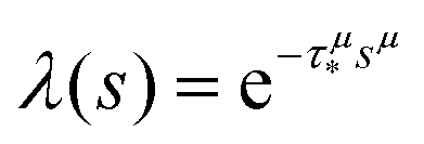
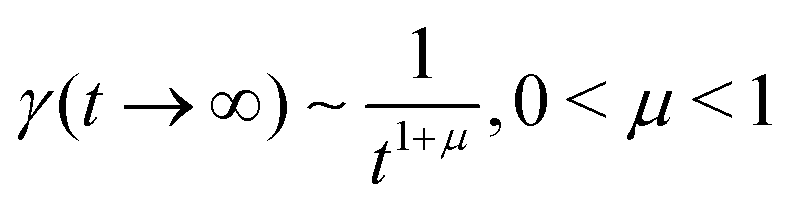
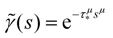
In order to simulate the exciton diffusion, we used a discrete random walk on the 2D square lattice. The finite N × N lattice with periodic boundary conditions was used. At every step, the simulated particle performs jumps to the nearest neighbours (see Fig. 1) with equal probability 1/4. The surface defects (traps) were fixed at the left-down corner of the lattice while the initial exciton position was sampled from a discrete uniform random distribution. The time Δt of the jump along the lattice was modelled by a constant value much smaller than the time scale of photoluminescence and trapping processes. The exciton in a free state can recombine with a probability p at each jump, i.e. we neglect any interactions between the excitons, which is perfectly justified for low-to-moderate intensities of an initial laser pulse.51 The trapping occurs with the unit probability when the exciton reaches the trap position. Importantly, in our model, the probability distribution of trapping times is non-exponential, having a power-law tail such that the mean trapping time is infinite. Such trapping or waiting time distributions appear in the theory of transport in disordered media called the Continuous Time Random Walk model,45,52,53 other literature54–56 and references therein. This distribution of trapping times occurs, for instance, in systems with an exponential distribution of depths of potential wells.57 We sample the trapping times from the one-sided α-stable distribution with the Lévy index μ, 0 < μ < 1.58 Such a distribution possesses long time asymptotics γ(t) ∼ t−1−μ. The Laplace transform of the distribution reads  . In simulations, we use τ* = 1 ns, and to gain more information about α-stable distributions, see Appendix A. After a particle escapes from the trap, it can be trapped again, i.e. the multiple trapping of excitons is taken into account by the model.
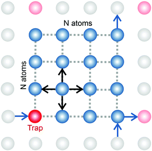 |
| | Fig. 1 In our simulations, we used a model of a random walk on a 2D square lattice modelled as an N × N set of vertices (atoms) with periodic boundary conditions. The jump probabilities are equal in four directions. Some of the vertices are capable of trapping an exciton with a heavy-tail distribution of trapping times,  . If an exciton jumps on the trap position, it gets bound to the site until it escapes. The recombination is modelled by decay probability p per step. . If an exciton jumps on the trap position, it gets bound to the site until it escapes. The recombination is modelled by decay probability p per step. | |
As a result, the motion of an exciton in our model is characterised by a normal diffusive (Brownian) motion at short times and a subdiffusion with a characteristic power-law exponent μ at long times. Fig. 2 shows the dependence of an exciton mean-squared displacement as a function of time in the absence of decay. Indeed, at first, the particles diffuse freely, but then the trapping and a subsequent release become important and the effective motion becomes subdiffusive.
 |
| | Fig. 2 Mean-squared displacement for exciton diffusion as a function of time on a double logarithmic scale in the absence of decay. The transition from a normal diffusive regime to subdiffusion is observed. The red curve corresponds to the parameters we use for core structures, i.e. the simulations were performed on a 15 × 15 periodic lattice (i.e. 1 defect per 225 sites), the exponent for trapping times was μ = 0.8 and the step duration Δt = 1 ps. The green curve stands for core–shell NPLs and we used the 10 × 10 periodic lattice (i.e. 1 defect per 100 sites), the exponent for trapping times was μ = 0.8 and the step duration Δt = 1 ps. The curves were obtained by ensemble averaging over 1000 trajectories. The numbers 1.0 and 0.8 show the corresponding slopes. | |
The photoluminescence intensity is defined by the number of exciton recombinations per second, i.e. by the distribution of recombination times. In simulations, we obtained this distribution from the set of Nsim independent runs, i.e. we again used a low exciton density assumption. The normalised emission intensity was calculated by aggregation of the single recombination (photoluminescence) events in the bins of size tbin (corresponding to the time resolution in the experiment32) and further normalisation by the number of events in the first bin in the spirit of experimental work.32 The middle of the corresponding bin was used as a time coordinate for the normalised emission intensity. Thus, our tbin corresponds to the exposition time in the experiment.32 An increase of tbin leads to noise reduction on the one hand and to smoothing of the curve and possible loss of fine effects on the other hand. Another important fact is that the highest intensity of PL occurs at short times. Hence, by enlarging the bin, one gets disproportionately high counts for the first bin. In the latter case, we effectively decrease the rest of the values.
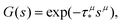
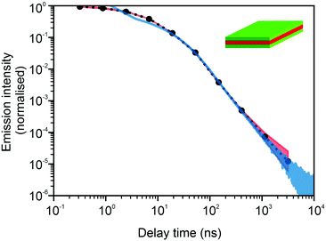
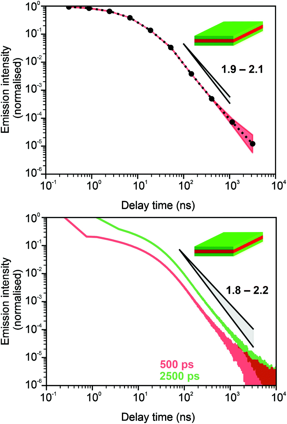
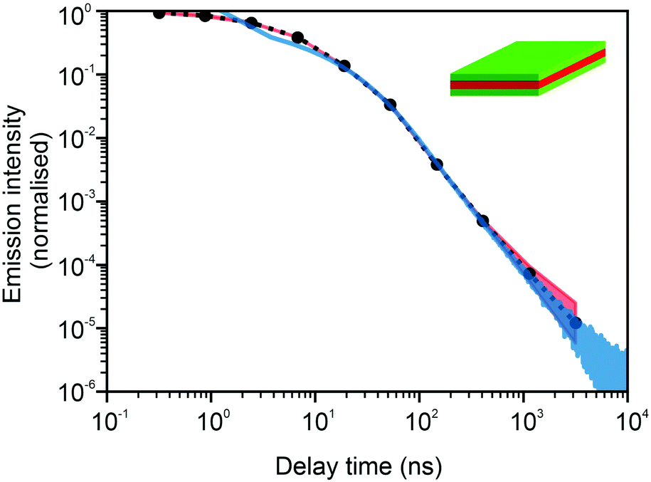
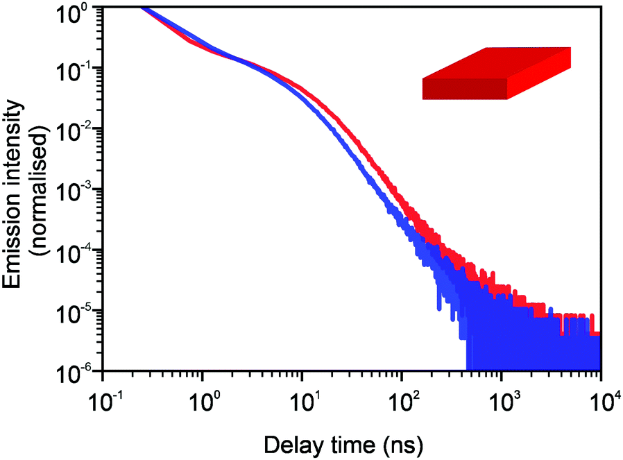
In Fig. 3 and 4, we show the comparison of our simulation model with fitted parameters (bottom plots) with experimental data for the photoluminescence intensity reported in ref. 32 (upper plots). Fig. 3 shows the PL intensity for core CdSe NPLs and Fig. 4 shows the PL intensity for core–shell CdSe–CdS nanoplatelets with CdS forming the outer layers. In order to plot and analyse the experimental data, we have used the plots from the ESI of ref. 32 and digitised the data with the help of the GetData Graph Digitizer program.59 Black dots in the upper plots of Fig. 3 and 4 are the averages of the digitised data with the red region representing the statistical error of measurements. One can see that the power laws including the intermediate ones nicely match between the simulations and experiments. For both the simulation results and the experimental results of ref. 32, we show the range in exponents in order to show how sensitive they are to the size of the interval that visually looks “straight”. By showing the results for two different bin sizes in the simulations, we illustrate that while the long time power-law asymptotics stays the same, the intermediate one is affected by renormalisation. This pushes us to the conclusion that the intermediate power laws are transitive phenomena rather than true power laws. Moreover, the adjustment of the bin in simulations could produce a very good quantitative match with experimental data (see Appendix B). However, we discovered that the experimental data consist of two differently normalised parts (see the ESI of ref. 32) and also reveal a range of values for power law asymptotics depending on the time interval chosen for averaging. Hence, we focus here on the explanation of the power laws rather than on an attempt to match the data quantitatively.
 |
| | Fig. 3 Comparison of digitised experimental data taken from the ESI of ref. 32 (corresponding to Fig. 1c in the main text of the reference) (above) with the simulation curves (below) for the case of core CdSe NPLs. The simulations were performed on the 15 × 15 periodic lattice (i.e. 1 defect per 225 sites), the exponent for trapping times was μ = 0.8, the step duration Δt = 1 ps and the probability of recombination per step p = 10−3. Nsim = 107. Two different binnings are shown in the plot with simulation data. The green curve corresponds to tbin = 2500 ps while the red curve is for tbin = 500 ps. We have recalculated the slopes from Fig. 1c in ref. 32. For both experiments and simulations, we show the range of slopes obtained with the least mean squares method applied to different subintervals of a seemingly straight part of the dependence. | |
 |
| | Fig. 4 Comparison of digitised experimental data taken from the ESI of ref. 32 (corresponding to Fig. 2g in the main text) (above) with the simulation curves (below) for the case of core–shell CdSe–CdS NPLs with CdS forming the outer layers. The simulations were performed on a 10 × 10 periodic lattice (i.e. 1 defect per 100 sites), the exponent for trapping times was μ = 0.8, the step duration Δt = 1 ps and the probability of recombination per step p = 10−3. Nsim = 107. The green curve in the bottom plot corresponds to tbin = 2500 ps while the red curve is for tbin = 500 ps. We assume that defects are concentrated on the outer surface of CdS. This explains a different selection of trap density in our simulation model for this case (cf.Fig. 3). We have recalculated the slopes from Fig. 2g in ref. 32 and for both experiments and simulations, we show the range of slopes obtained with the least mean squares method applied to different subintervals of a seemingly straight part of the dependence. | |
Note that we were not able to get a good match of the overall curve shapes with experiments for the core–crown case from ref. 32 (still, the long time power-law tail can be easily reproduced). We believe that the reason for this is that this case is markedly different. In comparison to the pure core or core–shell cases, it stands out as a system with a surface divided into two chemically distinctive areas with different properties. This obviously strongly affects the intermediate time scales. Hence, this case would require a more complex modelling approach.
The NPLs studied in experiments normally have a thickness of a few atomic layers. Hence, diffusion into inner layers is also possible. If one takes into account these bulk layers, the results stay qualitatively the same, as shown in Appendix C.
3 Theoretical model. Non-Markovian kinetic rate equations
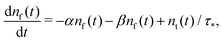
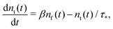
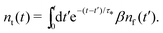
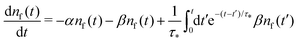
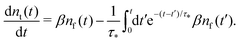
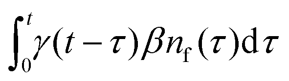
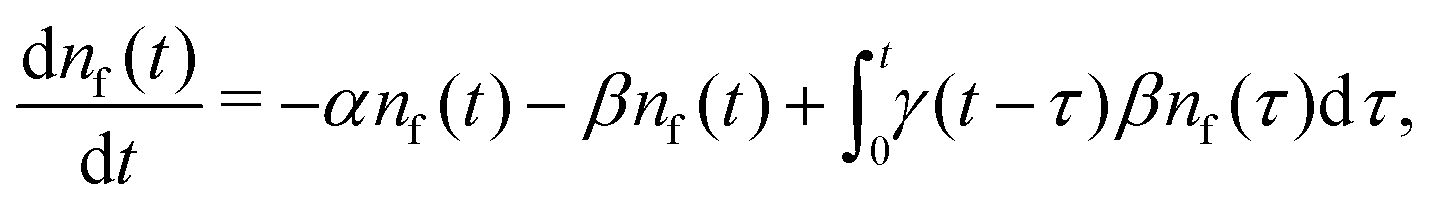
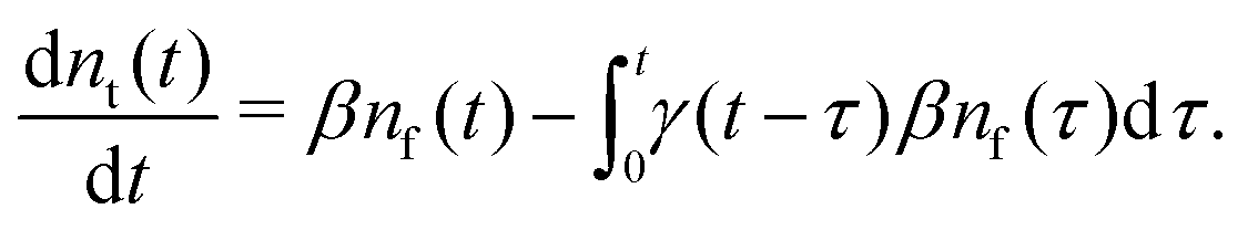
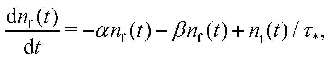
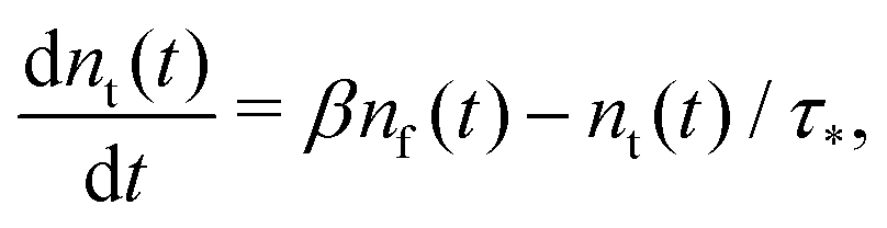
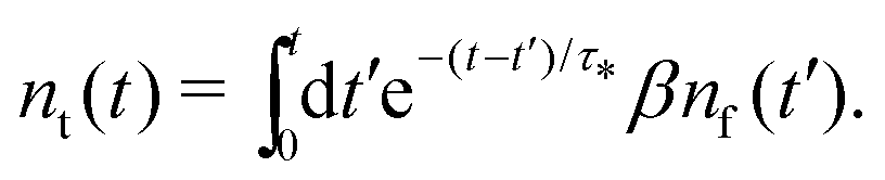
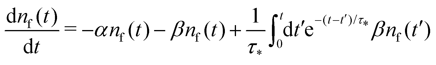
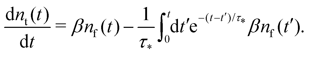
Our theoretical model corresponds to the simulation setup with one simplification. We additionally assume that at every step, the trapping happens at a constant rate β and is proportional to the number of particles in the free state βnf(t), with nf(t) being the number of excitons in the free state as a function of time t. This coefficient β effectively describes the diffusion of excitons and can be connected to properties of the simulation model (see below). The decay (recombination) is assumed to be proportional to the concentration nf(t) as αnf(t), where α is the rate of the recombination process. Eventually, an exciton escapes the trapped state and switches back to the diffusion-decay mode. For the population of excitons in the diffusive state, the trapping process presents a temporary loss with a delayed return. This return can be described by a term with the kernel γ(t − τ),  , where t is a release time moment as compared to τ, the time of the trapping event. The kernel has an explicit meaning of trapping probability density as a function of time, i.e. it abides a normalisation property,
  . Hence, our theoretical model describes the recombination-caused photoluminiscence process as a two-state system model with only one of the states allowing the recombination.
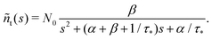
Summarising the above model in terms of kinetic rate equations for concentrations of free excitons nf(t) and the trapped excitons nt(t), one gets
| |  | (1) |
| | 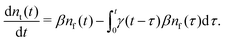 | (2) |
The initial conditions are
nf(0) =
N0,
nt(0) = 0,
i.e. the laser excitation produces
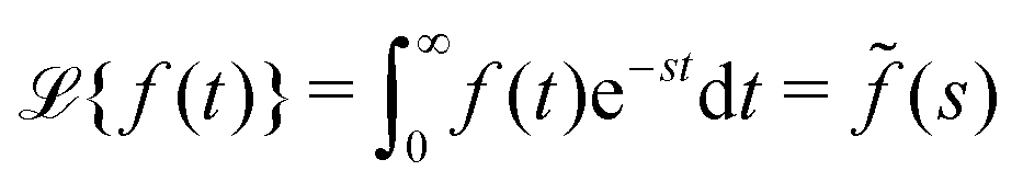
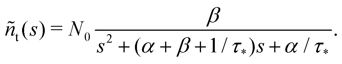
N0 particles in the free state, but no trapped ones. Applying the Laplace transform
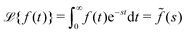
turns the equations into algebraic ones. The solution for
ñf(
s) reads
| | 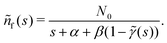 | (3) |
Since
γ(
t) is normalised, 1 −
![[small gamma, Greek, tilde]](https://www.rsc.org/images/entities/i_char_e0dd.gif)
(
s) never becomes negative and any possible divergencies are avoided. Also, it can be proven that the solution
nf(
t) is non-negative at all times (Appendix D). Clearly, in a general case, the system of
eqn (1) and (2) describes a non-Markovian process due to the memory kernel. The Markovian case can be obtained for the particular case of an exponential distribution of trapping times (for more details and the exact solution of that case, see Appendices E and F). We assume that the power law tails observed in experiments appear due to the power law asymptotics of trapping times,
i.e. one can use an α-stable law for the kernel,

, 0 <
μ < 1. In the limit of long times
t → ∞ (which corresponds to
s → 0), the function

. Thus, in this limit, the concentration of freely diffusing excitons is
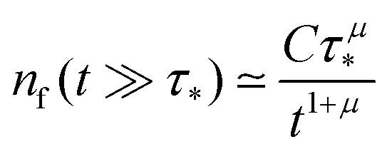
| | 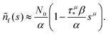 | (4) |
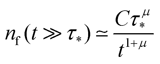
This expression produces a long-time power-law asymptotics,
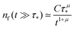
, with
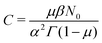
(see the derivation in Appendix G). Then, the limit expression for the emission intensity is
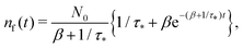
| |  | (5) |
In order to compare the theoretical model with the simulations, we need to find the correspondence between the simulation parameters and the constants used in the theory. As a test example, we use the simulation results from Fig. 3 with the following parameters: the simulation step Δt is 1 ps, the bin size is 500 ps, the time limit of the simulation is 10![[thin space (1/6-em)]](https://www.rsc.org/images/entities/char_2009.gif) 000 ns, a 2D square lattice with 1 defect per 15 × 15 = 225 points, μ = 0.8, and the probability of recombination per step is 10−3. Hence, the parameters to be put in eqn (3) can be estimated as follows. For
000 ns, a 2D square lattice with 1 defect per 15 × 15 = 225 points, μ = 0.8, and the probability of recombination per step is 10−3. Hence, the parameters to be put in eqn (3) can be estimated as follows. For  , the coefficients are μ = 0.8 and τ* = 1 ns. The rate of recombination α can be determined as a probability of recombination per step divided by the step's duration, i.e. α = 1 ns−1. The rate of exciton capture by defects (traps) β is roughly the probability of finding a defect per step. This probability equals 1/225 if one neglects the effect of secondary trapping in which case the probability of being caught by the defect is higher after escape from a defect. For the case of the first trapping event, the value of the probability is based on the fact that original excitations occur homogeneously in the sample. For the first trapping case, βfirsttrap can be then estimated as
 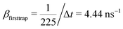 (the trapping rate is almost constant at short times). In order to account for the undercounting of trapping events at long times in our theoretical model, we slightly increase the trapping rate and set β = 7.5 ns−1. At long times, secondary trapping is quite likely since right after escape from a trap, a particle is more likely to come back than at earlier times.
Fig. 5 shows the excellent correspondence between the theoretical and simulation results obtained for these parameters. Since the simulation results are normalised on the first bin, the theoretical curve was scaled such that the first points roughly coincide.
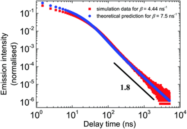 |
| | Fig. 5 The outcome of the theoretical model vs. the simulation results in the double log scale for all relevant time scales. The parameters of the theory are β = 7.5 ns−1, α = 1 ns−1, and μ = 0.8. In simulations, β = 4.44. Red dots correspond to the simulation data. Blue points are the numerical inverse Laplace transform of eqn (3). tbin = 500 ps. | |
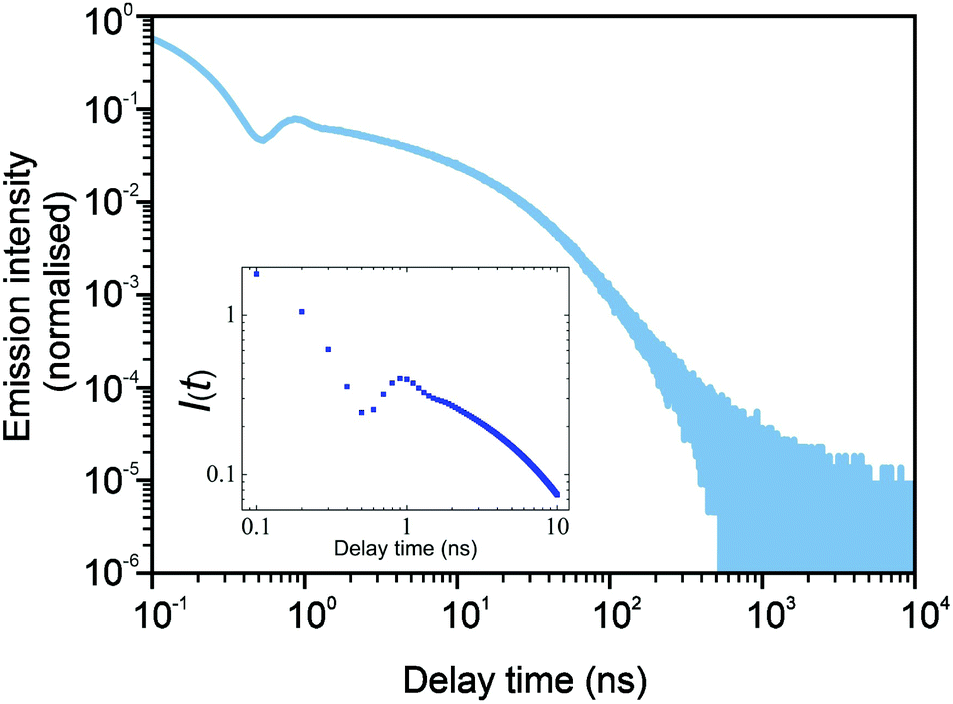
The study of parameter space both in simulation and theoretical models shows that at intermediate times, a rich behaviour can be observed. In Fig. 6, for the chosen parameters, the curve weekly oscillates, which is a result of an interplay of trapping, release and recombination terms both in simulations (the main plot) and in theory (the inset).
 |
| | Fig. 6 The simulation results (the main plot) with fine binning showing the same intermediate fluctuating behaviour as in the theoretical model (shown in the inset). Here, the bin size was chosen to be tbin = 25 ps, μ = 0.8, p = 10−3, and Nsim = 107, and one trap was put per 100 lattice sites. | |
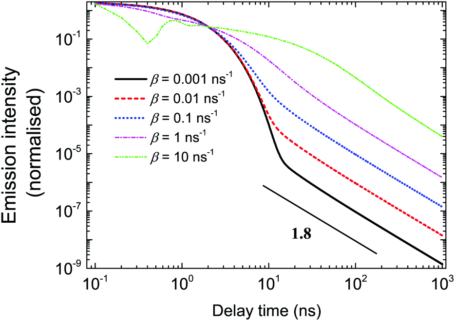
The shapes of the emission intensity curves are defined by the interplay between free diffusion, trapping and recombination of excitons. One can see from Fig. 7 that the overall shape is controlled by diffusion properties. For any set of parameters at short times, emission is defined by recombination only and the intensity decays exponentially. The latter observation was made experimentally, e.g. see ref. 27. Exponential decay at short times also follows from eqn (3). At large s, which corresponds to the short time domain, ñf(s) ∼ N0/(s + α + β), that is, nf(t) ∼ N0exp(−(α + β)t). At short times, most of the excitons are free. In the course of time, they get trapped, and they escape the traps later. Since the trapping times are described by a power-law with exponent μ + 1 at long times, the emission is defined by the release of excitons and characterised by the same power-law. The parameter β defines both the duration of the short time limit and the properties of the transition region. At small β (slow diffusion), the transition from exponential to power-law decay happens without a noticeable transition region (see the black solid curve in Fig. 7). Then, with a growth of β, the intermediate region appears, which is well illustrated by the pink dash-dotted curve in Fig. 7. This is a regime where intermediate power laws were suggested in ref. 32. Finally, for fast diffusion (green dash dot-dotted curve in Fig. 7), one can observe a wide transition region with oscillations of emission intensity. These oscillations could be associated with multiple trapping and release events.
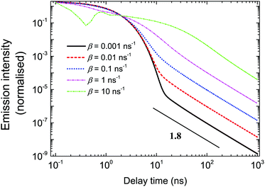 |
| | Fig. 7 Dependence of logarithm of emission intensity as a function of logarithm of time for different β. The parameter β is defined by the free diffusion coefficient of excitons. The variation of β leads to a change in the characteristic shape of the emission intensity curves. | |
4 Summary
We proposed a diffusion-based simulation model and non-Markovian kinetic rate equations with a delay function, which describe the interplay between free diffusion, trapping and recombination of excitons in 2D semiconductor nanostructures. The parameters of both models have a clear physical interpretation. The models were applied for the interpretation of experimental data on photoluminescence kinetics in CdSe/CdS core and core–shell nanoplatelets. The characteristic power-law tails are the result of exciton escape properties from surface defect traps. We show that the intermediate power laws found in ref. 32 are transitional effects rather than true power-law dependencies. Moreover, we see that diffusion properties control the emission intensity in the intermediate region between the simple exponential decay at short times and a power-law at long times. The duration and the features of this intermediate region vary substantially with the value of diffusivity. In particular, in the case of a fast diffusion complex, oscillating dependencies are demonstrated. The proposed model can be applied for the analysis of exciton kinetics in semiconductor nanoplatelets (core, core–shell, core–crown) and for the estimation of microscopic exciton parameters. In Appendix C, we show a possible pathway for the model generalisation for the 3D case. Further generalisations of the proposed model and additional assumptions may be necessary to use the model for other low-dimensional semiconductor structures.
Conflicts of interest
There are no conflicts to declare.
Appendix A: α-stable Lévy laws
In our model, we choose a one-sided (completely asymmetric) α-stable Lévy distribution as a model distribution for the statistics of trapping times. The reasons for that are both mathematical and practical.
Mathematically, according to the generalised central limit theorem, the distribution of the properly normalised sum of independent identically distributed variables converges to an α-stable Lévy law if the variables are drawn from a distribution with a divergent second moment.60 The α-stable distributions can only be written analytically in terms of often hard-to-grasp Fox H-functions with three exceptions (Gaussian, Cauchy and Lévy-Smirnov distributions). However, their Fourier/Laplace transforms adopt a simpler stretched Gaussian/exponential form, as reported in ref. 61. In the case of trapping time distributions, the quantities adopt positive values only, i.e. one needs to consider a particular case of one-sided alpha-stable distributions. For the latter, the Laplace transform reads
| |  | (6) |
where 0 <
μ ≤ 1,
s ∈ [0,∞). At long times, this distribution exhibits a power-law asymptotics that decays (up to a numerical prefactor) as

.
The practical reason for our choice is a convenience of working with exponential dependencies both in terms of expansions and numerical calculations. In simulations, the distribution was sampled according to ref. 58.
Appendix B: match between theory and experiment for the binning value tbin = 2.5 ns
If one plots the simulation and experimental results from Fig. 4 for the binning 2.5 ns = 2500 ps, one finds a very good quantitative match (Fig. 8). However, one has to keep in mind that the values depend on the normalisation that was not always known from experimental data in ref. 32.
 |
| | Fig. 8 Quantitative match for photoluminescence intensities between the simulations and experiments as reported in ref. 32 for the binning tbin = 2.5 ns for the case of core–shell CdSe–CdS NPLs with CdS forming the outer layers. | |
Appendix C: modelling the process in a few atomistic layers
For the 3D model, half of the NPL vs. the symmetry plane parallel to the surface was simulated with Nl layers (N × N × Nl). The traps are located only in the surface layer. Periodic boundary conditions are applied to in-plane coordinates. The initial exciton positions are generated from discrete uniform distributions along all three coordinates. The exciton cannot escape to the solution, so the possible jumps on the surface layer (N, N, 0) are [(+1, 0, 0), (−1, 0, 0), (0, +1, 0), (0, −1, 0), (0, 0, +1)] with equal probabilities of 1/5. In the internal layer, the possible jumps are [(+1, 0, 0), (−1, 0, 0), (0, +1, 0), (0, −1, 0), (0, 0, +1), (0, 0, −1)] with equal probabilities of 1/6. In order to account for the symmetry of the NPL, the crossing of the symmetry plane (0, 0, +1) is replaced by (0, 0, 0) for even Nl (2Nl layers in NPL) or by (0, 0, −1) for the odd Nl (2(Nl − 1) + 1 layers in NPL).
In Fig. 9, we see that for core NPLs, the 2D model and the model of diffusion in a few parallel atomistic layers give the same results. In this case, we assume the density of surface defects to be the same as it was in Fig. 3, i.e. 1 defect per 225 surface lattice sites. Fig. 10 shows the comparison of the three different models. Namely, the 2D model, the 3D model that assumes the same properties and jump probabilities in all 5 layers and the 3D model where jump probabilities differ when the jumps occur from the surface layers into the bulk. The latter case is the easiest generalisation of a 3D model. It assumes that the jumps into the bulk and back to the surface are 5 times less likely than the jumps within the same layer. The density of defects corresponds to Fig. 4, i.e. 1 per 100 surface lattice sites. All three curves show the same tail behaviour as one would expect. The transitional region changes its shape and shifts, i.e. more complex models allow for a finer description. We see that the available experimental data can be fitted well with a relatively simple 2D approach, which tells us that the 2D model is sufficient as a minimal model.
 |
| | Fig. 9 Comparison of curves for photoluminescence intensities for 2D (red) and 3D (blue) models. The core case is shown with a density of defects 1 per 225 surface lattice sites. μ = 0.8, Nsim = 106, and tbin = 500 ps. | |
 |
| | Fig. 10 Comparison of curves for photoluminescence intensities for 2D (red), 3D homogeneous (blue) and 3D distinct domain (cyan) models. The core–shell case is shown with a density of defects of 1 per 100 surface lattice sites. μ = 0.8, Nsim = 106, and tbin = 500 ps. The kink at short times occurs due to binning. In the first two cases, the jumps are considered to be equally likely for all directions. For the last case (cyan data), the layers are split between two regions. The outer region represents one material and the inner region represents another one. Thus, it corresponds to the core–shell structure more realistically. The jumps from the surface layer into the bulk layers and back are 5 times less likely than the probabilities of jumps within the same region. | |
Appendix D: proof of the non-negativity of eqn (1) solutions
The concentration of excitons must be non-negative. Hence, according to the Bernstein theorem,62 its Laplace transform ñf(s) should be completely monotonic (c.m.). The function ![[g with combining tilde]](https://www.rsc.org/images/entities/i_char_0067_0303.gif) (s) is called c.m. if (−1)n(n)(s) ≥ 1 for s > 0 and n = 0, 1, 2,…. If m1(s) and m2(s) are completely monotonic, then their product m1(s)m2(s) is also c.m. Also, if
(s) is called c.m. if (−1)n(n)(s) ≥ 1 for s > 0 and n = 0, 1, 2,…. If m1(s) and m2(s) are completely monotonic, then their product m1(s)m2(s) is also c.m. Also, if ![[f with combining tilde]](https://www.rsc.org/images/entities/i_char_0066_0303.gif) (s) is c.m. and
(s) is c.m. and ![[h with combining tilde]](https://www.rsc.org/images/entities/i_char_0068_0303.gif) (s) is the Bernstein function (i.e. ≥ 0 for positive s and ′(s) is c.m.), then ((s)) is c.m.62
(s) is the Bernstein function (i.e. ≥ 0 for positive s and ′(s) is c.m.), then ((s)) is c.m.62
In order to show the complete monotonicity of ñf(s), we present it as ñf(s) = ((s)), where = 1/s and (s) = s + α + β(1 − (s)). The function (s) is positive since (s) is the Laplace transform of the probability distribution function and, therefore, (s) ≤ 1. The function (s) is c.m. as the Laplace transform of the PDF, i.e. (−1)n(n)(s), ≥ 0. The derivative ′(s) = 1 − β′(s) is c.m. since (s) is c.m. Thus, due to the property mentioned above, ñf(s) = ((s)) is c.m. as well and nf(t) is non-negative due to the Bernstein theorem.62
Appendix E: the derivation of the limit result for the two state Markovian limit
We show here how one can recover the limit of a two state Markovian system with constant rates of exchange and a decay in one of the states (considered, for instance, in Van Kampen's book,63 Chapter VII, Section 5, exercise (5.8)). This corresponds to the Markovian limit of eqn (1) and (2).
The case of two states with exchange can be written as
| |  | (7) |
| |  | (8) |
where
nf(
t) and
nt(
t) correspond to the free and trapped states in our model and
α,
β and
τ* are positive constants.
Let us treat eqn (8) formally as a non-homogeneous ordinary differential equation of the first order. Then, its formal solution reads
| |  | (9) |
By substituting the last equation into (7), we get
| |  | (10) |
and, respectively,
| |  | (11) |
We see that the system of eqn (10) and (11) is a particular case of our model eqn (1) and (2) with the exponential trapping PDF 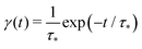 . Thus, we have established a link of the non-Markovian model (1)–(2) and the classical Markovian two-state equations.63
Appendix F: solution of Markovian kinetic rate equations
We consider eqn (7) and (8) with initial conditions nf(t = 0) = N0 and nt(t = 0) = 0. In the Laplace space,| | | sñf − N0 = −αñf − βñf + ñt/τ*, | (12) |
or| | | (s + α + β)ñf − ñt/τ* = N0, | (14) |
| | | −βñf + (s + 1/τ*)ñt = 0. | (15) |
Determinant| | | Det = s2 + (α + β + 1/τ*)s + α/τ*. | (16) |
The solution reads| |  | (17) |
| |  | (18) |
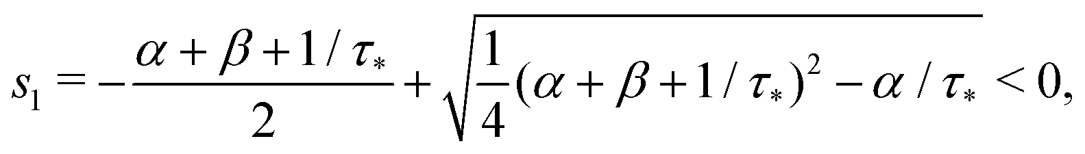
The denominator can be written as| | | s2 + (α + β + 1/τ*)s + α/τ* = (s + |s1|)(s + |s2|), | (19) |
where s1 and s2 are the roots of the quadratic equation| | | s2 + (α + β + 1/τ*)s + α/τ* = 0, | (20) |
that is
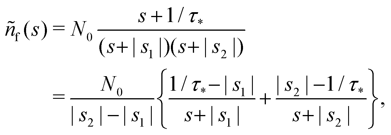
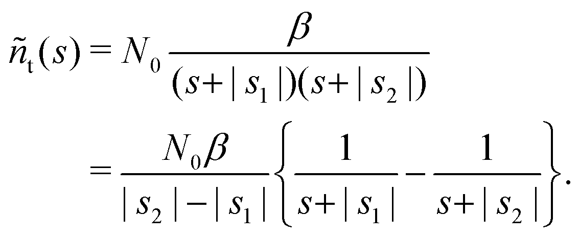
After plugging (19) into (17) and (18), we get
| |  | (21) |
| | 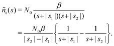 | (22) |
Taking the inverse Laplace transform
| | 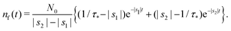 | (23) |
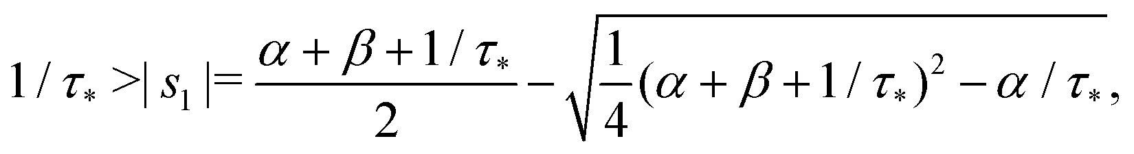
| |  | (24) |
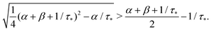
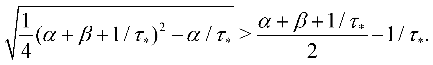
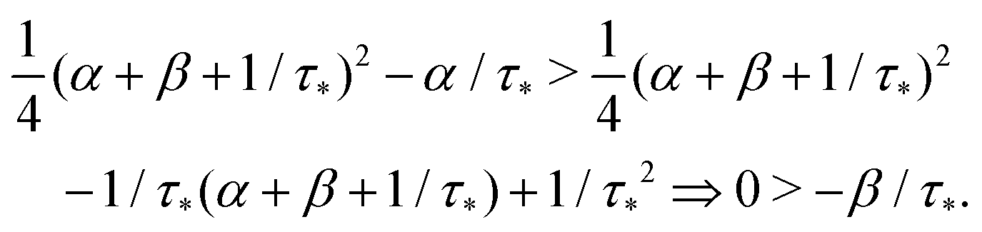
Remark 1. It is possible to prove that |s1| < 1/τ* < |s2|, thus both terms in the brackets of (23) are positive and, automatically, the term in the brackets of (24) are also positive. For example,
| |  | (25) |
| |  | (26) |
If α + β < 1/τ*, then the left side >0, and the right side <0. If α + β > 1/τ*, then taking square of both sides,
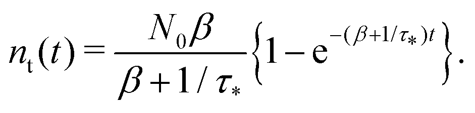
In the same way, the inequality 1/τ* < |s2| is proved.
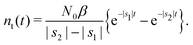
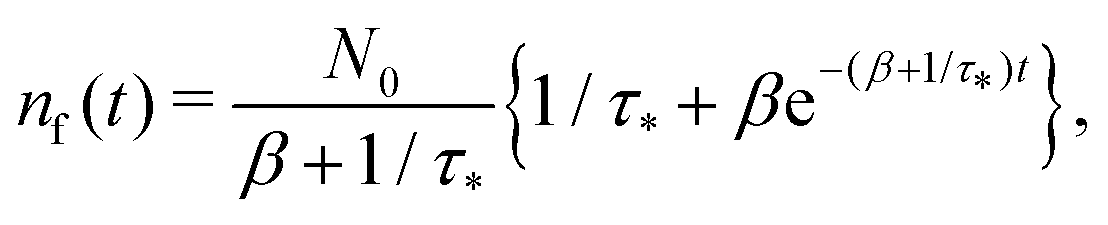
Remark 2. If α = 0, then s1 = 0, s2 = −(β + 1/τ*), and then nf(t) and nt(t) reduce to
| |  | (27) |
| |  | (28) |
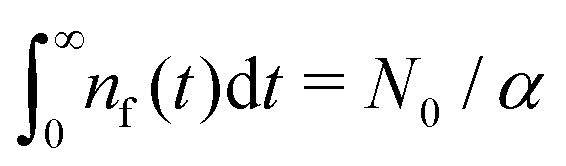
Remark 3. Normalisation. ñf(s = 0) = N0/α = const. This implies normalisation 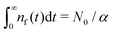 that follows directly from eqn (3).
Appendix F: derivation of the asymptotic power-law for nf(t)
In order to derive eqn (5) for the emission intensity in the long-time limit, we follow the reasoning from ref. 64 and use an identity| | 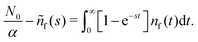 | (29) |
From the expansion of ñf(s) at small s, in eqn (4), we infer that nf(t) decays at long times as  . We put the latter expression in the identity and get
| | 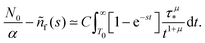 | (30) |
Now, we take derivatives from both sides with respect to s and using the Tauberian theorem for Laplace transforms,62 we get| | 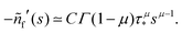 | (31) |
After differentiating eqn (4), one obtains the expression for C,| | 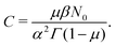 | (32) |
Acknowledgements
The authors would like to acknowledge the support of the Russian Science Foundation project no. 18-72-10002 as well as fruitful discussions with Igor M. Sokolov.
Notes and references
-
E. L. Ivchenko, Optical Spectroscopy of Semiconductor Nanostructures, Alpha Science Int., Harrow, UK, 2005 Search PubMed.
- V. L. Colvin, M. C. Schlamp and A. P. Alivisatos, Nature, 1994, 370, 354–357 CrossRef CAS.
- V. I. Klimov, A. A. Mikhailovsky, S. Xu, A. Malko, J. A. Hollingsworth, C. A. Leatherdale, H. J. Eisler and M. G. Bawendi, Science, 2000, 290, 314–317 CrossRef CAS.
- A. Y. Nazzal, L. Qu, X. Peng and M. Xiao, Nano Lett., 2003, 3, 819–822 CrossRef CAS.
- S. Ithurria and B. Dubertret, J. Am. Chem. Soc., 2008, 130, 16504–16505 CrossRef CAS.
- M. Xu, T. Liang, M. Shi and H. Chen, Chem. Rev., 2013, 113, 3766–3798 CrossRef CAS.
- R. Benchamekh, N. A. Gippius, J. Even, M. O. Nestoklon, J.-M. Jancu, S. Ithurria, B. Dubertret, A. L. Efros and P. Voisin, Phys. Rev. B: Condens. Matter Mater. Phys., 2014, 89, 035307 CrossRef.
- J. Q. Grim, S. Christodoulou, F. D. Stasio, R. Krahne, R. Cingolani, L. Manna and I. Moreels, Nat. Nanotechnol., 2014, 9, 891–895 CrossRef CAS.
- A. W. Achtstein, A. Schliwa, A. Prudnikau, M. Hardzei, M. V. Artemyev, C. Thomsen and U. Woggon, Nano Lett., 2012, 12, 3151–3157 CrossRef CAS.
- S. Ithurria, M. D. Tessier, B. Mahler, R. P. Lobo, B. Dubertret and A. L. Efros, Nat. Mater., 2011, 10, 936–941 CrossRef CAS.
- B. Mahler, B. Nadal, C. Bouet, G. Patriarche and B. Dubertret, J. Am. Chem. Soc., 2012, 134, 18591–18598 CrossRef CAS.
- M. D. Tessier, P. Spinicelli, D. Dupont, G. Patriarche, S. Ithurria and B. Dubertret, Nano Lett., 2014, 14, 207–213 CrossRef CAS.
- L. Biadala, F. Liu, M. D. Tessier, D. R. Yakovlev, B. Dubertret and M. Bayer, Nano Lett., 2014, 14, 1134–1139 CrossRef CAS.
- M. Pelton, S. Ithurria, R. Schaller, D. Dolzhnikov and D. V. Talapin, Nano Lett., 2012, 12, 6158–6163 CrossRef CAS.
- C. She, I. Fedin, D. S. Dolzhnikov, A. Demortiere, R. D. Schaller, M. Pelton and D. V. Talapin, Nano Lett., 2014, 14, 2772–2777 CrossRef CAS.
- B. Guzelturk, Y. Kelestemur, M. Olutas, S. Delikanli, H. V. Schaller and A. Demir, ACS Nano, 2014, 8, 6599–6605 CrossRef CAS.
- M. J. Bruchez, M. Moronne, P. Gin, S. Weiss and A. P. Alivisatos, Science, 1998, 281, 2013–2016 CrossRef CAS.
- L. Manna, D. J. Milliron, A. Meisel, E. C. Scher and A. P. Alivisatos, Nat. Mater., 2003, 2, 382–385 CrossRef CAS.
- C. B. Murray, D. J. Norris and M. G. Bawendi, J. Am. Chem. Soc., 1993, 115, 8706–8715 CrossRef CAS.
- X. Michalet, F. F. Pinaud, L. A. Bentolila, J. M. Tsay, S. Doose, J. J. Li, G. Sundaresan, A. M. Wu, S. S. Gambhir and S. Weiss, Science, 2005, 307, 538–544 CrossRef CAS.
- A. M. Smirnov, A. D. Golinskaya, P. A. Kotin, S. G. Dorofeev, V. V. Palyulin, V. N. Mantsevich and V. S. Dneprovskii, J. Lumin., 2019, 213, 29–35 CrossRef CAS.
- A. M. Smirnov, A. D. Golinskaya, P. A. Kotin, S. G. Dorofeev, E. V. Zharkova, V. V. Palyulin, V. N. Mantsevich and V. S. Dneprovskii, J. Phys. Chem. C, 2019, 123, 27986–27992 CrossRef CAS.
- M. Nasilowski, B. Mahler, E. Lhuillier, S. Ithurria and B. Dubertret, Chem. Rev., 2016, 116, 10934–10982 CrossRef CAS.
- J. Owen, Science, 2015, 347, 615–616 CrossRef CAS.
- M. A. Boles, D. Ling, T. Hyeon and D. V. Talapin, Nat. Mater., 2016, 15, 141–153 CrossRef CAS.
- J. Owen and L. Brus, J. Am. Chem. Soc., 2017, 139, 10939–10943 CrossRef CAS.
- L. Biadala, E. V. Shornikova, A. V. Rodina, D. R. Yakovlev, B. Siebers, T. Aubert, M. Nasilowski, Z. Hens, B. Dubertret, A. L. Efros and M. Bayer, Nat. Nanotechnol., 2017, 12, 569–574 CrossRef CAS.
- M. Nirmal, B. O. Dabbousi, M. G. Bawendi, J. J. Macklin, J. K. Trautman, T. D. Harris and L. E. Brus, Nature, 1996, 383, 802 CrossRef CAS.
- U. Banin, M. Bruchez, A. P. Alivisatos, T. Ha, S. Weiss and D. S. Chemla, J. Chem. Phys., 1999, 110, 1195–1201 CrossRef CAS.
- M. Kuno, D. P. Fromm, H. F. Hamann, A. Gallagher and D. J. Nesbitt, J. Chem. Phys., 2001, 115, 1028–1040 CrossRef CAS.
- F. D. Stefani, J. P. Hoogenboom and E. Barkai, Phys. Today, 2009, 62, 34 CrossRef CAS.
- F. T. Rabouw, J. C. van der Bok, P. Spinicelli, B. Mahler, M. Nasilowski, S. Pedetti, B. Dubertret and A. Vanmaekelbergh, Nano Lett., 2016, 16, 2047–2053 CrossRef CAS.
- E. V. Shornikova, L. Biadala, D. R. Yakovlev, V. F. Sapega, Y. G. Kusrayev, A. A. Mitioglu, M. V. Ballottin, P. C. M. Christianen, V. V. Belykh, M. V. Kochiev, N. N. Sibeldin, A. A. Golovatenko, A. V. Rodina, N. A. Gippius, A. Kuntzmann, Y. Jiang, M. Nasilowski, B. Dubertret and M. Bayer, Nanoscale, 2018, 10, 646–656 RSC.
- M. Olutas, B. Guzelturk, Y. Kelestemur, A. Yeltik, S. Delikanli and H. V. Demir, ACS Nano, 2015, 9, 5041–5050 CrossRef CAS.
- F. T. Rabouw, M. Kamp, R. J. A. van Dijk-Moes, D. R. Gamelin, A. F. Koenderink, A. Meijerink and D. Vanmaekelbergh, Nano Lett., 2015, 15, 7718–7725 CrossRef CAS.
- L. T. Kunneman, J. M. Schins, S. Pedetti, H. Heuclin, F. C. Grozema, A. J. Houtepen and B. Dubertret, Nano Lett., 2014, 14, 7039–7045 CrossRef CAS.
- O. Del Pozo-Zamudio, S. Schwarz, M. Sich, I. A. Akimov, M. Bayer, R. C. Schofield, E. A. Chekhovich, B. J. Robinson, N. D. Kay, O. Kolosov, A. I. Dmitriev, G. V. Lashkarev, D. N. Borisenko, N. N. Kolesnikov and A. I. Tartakovskii, 2D Mater., 2015, 2, 035010 CrossRef.
- Q. Li and T. Lian, Nano Lett., 2017, 17, 3152–3158 CrossRef CAS.
- Q. Li, K. Wu, J. Chen, Z. Chen, J. R. McBride and T. Lian, ACS Nano, 2016, 10, 3843–3851 CrossRef CAS.
- M. C. Weidman, A. J. Goodman and W. A. Tisdale, Chem. Mater., 2017, 29, 5019–5030 CrossRef CAS.
- M. Kulig, J. Zipfel, P. Nagler, S. Blanter, C. Schüller, T. Korn, N. Paradiso, M. M. Glazov and A. Chernikov, Phys. Rev. Lett., 2018, 120, 207401 CrossRef CAS.
- J. Zipfel, M. Kulig, R. Perea-Causín, S. Brem, J. D. Ziegler, R. Rosati, T. Taniguchi, K. Watanabe, M. M. Glazov, E. Malic and A. Chernikov, Phys. Rev. B, 2020, 101, 115430 CrossRef CAS.
- M. M. Glazov, Phys. Rev. B, 2019, 100, 045426 CrossRef CAS.
- M. Seitz, A. J. Magdaleno, N. Alcazar-Cano, M. Melendez, T. J. Lubbers, S. W. Walraven, S. Pakdel, E. Prada, R. Delgado-Buscalioni and F. Prins, Nat. Commun., 2020, 11, 2035 CrossRef CAS.
- H. Scher and E. W. Montroll, Phys. Rev. B: Solid State, 1975, 12, 2455–2477 CrossRef CAS.
- B. Saidzhonov, V. Kozlovsky, V. Zaytsev and R. Vasiliev, J. Lumin., 2019, 209, 170 CrossRef CAS.
- T. Erdem and H. Demir, Nanophotonics, 2016, 5, 74 Search PubMed.
- B. Saidzhonov, V. Zaytsev, M. Berekchiian and R. Vasiliev, J. Lumin., 2020, 222, 117134 CrossRef CAS.
- A. Achtstein, O. Marquardt, R. Scott, M. Ibrahim, T. Riedl, A. Prudnikau, A. Antanovich, N. Owschimikow, J. Lindner, M. Artemyev and U. Woggon, ACS Nano, 2018, 12, 9476 CrossRef CAS.
- R. Scott, S. Kickhöfel, O. Schoeps, A. Antanovich, A. Prudnikau, A. Chuvilin, U. Woggon, M. Artemyev and A. Achtstein, Phys. Chem. Chem. Phys., 2016, 18, 3197 RSC.
- P. Irkhin and I. Biaggio, Phys. Rev. Lett., 2011, 107, 017402 CrossRef.
- E. W. Montroll and G. H. Weiss, J. Math. Phys., 1965, 6, 167–181 CrossRef.
- H. Scher and M. Lax, Phys. Rev. B: Solid State, 1973, 7, 4491–4502 CrossRef CAS.
-
B. D. Hughes, Random Walks and Random Environments, Clarendon Press, Oxford, UK, 1995, vol. 1 Search PubMed.
- J.-P. Bouchaud and A. Georges, Phys. Rep., 1990, 195, 127–293 CrossRef.
- R. Metzler and J. Klafter, Phys. Rep., 2000, 339, 1–77 CrossRef CAS.
- T. Tiedje and A. Rose, Solid State Commun., 1981, 37, 49–52 CrossRef CAS.
- J. M. Chambers, C. L. Mallows and B. W. Stuck, J. Am. Stat. Assoc., 1976, 71, 340–344 CrossRef.
- GetData Graph Digitizer program, http://getdata-graph-digitizer.com.
-
B. V. Gnedenko and A. N. Kolmogorov, Limit distributions for sums of independent random variables, Addison-Wesley Mathematics Series, Cambridge, UK, 1954 Search PubMed.
-
G. Samorodnitsky and M. S. Taqqu, Stable Non-Gaussian Random Processes: Stochastic Models with Infinite Variance, CRC Press, 1994 Search PubMed.
-
W. Feller, An Introduction to Probability Theory and Its Applications, Wiley, Cambridge, UK, 1991, vol. 2 Search PubMed.
-
N. G. Van Kampen, Stochastic Processes in Physics and Chemistry, Elsevier, 2007 Search PubMed.
- S. Havlin and G. H. Weiss, J. Stat. Phys., 1990, 58, 1267–1273 CrossRef.
|
| This journal is © the Owner Societies 2020 |
Click here to see how this site uses Cookies. View our privacy policy here. 
 Open Access Article
 This Open Access Article is licensed under a
  a,
V. N.
Mantsevich
b,
K. J.
Stevenson
a,
V. N.
Mantsevich
b,
K. J.
Stevenson
 . In simulations, we use τ* = 1 ns, and to gain more information about α-stable distributions, see Appendix A. After a particle escapes from the trap, it can be trapped again, i.e. the multiple trapping of excitons is taken into account by the model.
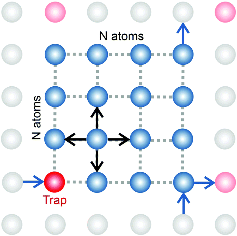
 . If an exciton jumps on the trap position, it gets bound to the site until it escapes. The recombination is modelled by decay probability p per step.
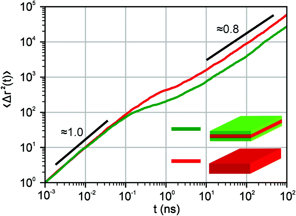

 , where t is a release time moment as compared to τ, the time of the trapping event. The kernel has an explicit meaning of trapping probability density as a function of time, i.e. it abides a normalisation property,
 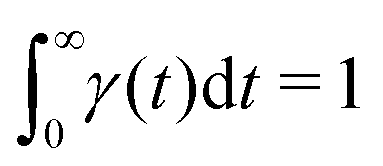 . Hence, our theoretical model describes the recombination-caused photoluminiscence process as a two-state system model with only one of the states allowing the recombination.
 turns the equations into algebraic ones. The solution for ñf(s) reads
 , 0 < μ < 1. In the limit of long times t → ∞ (which corresponds to s → 0), the function
 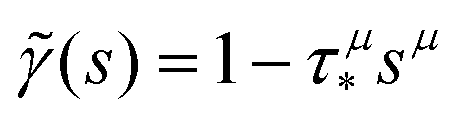 . Thus, in this limit, the concentration of freely diffusing excitons is
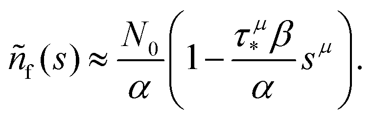
 , with
 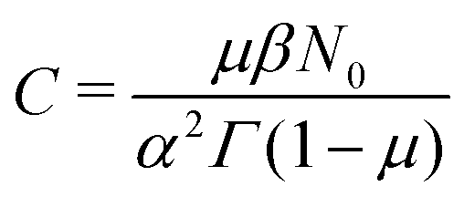 (see the derivation in Appendix G). Then, the limit expression for the emission intensity is
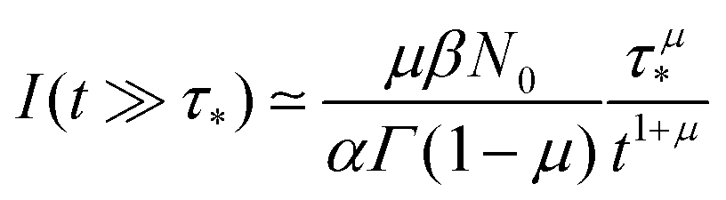
 , the coefficients are μ = 0.8 and τ* = 1 ns. The rate of recombination α can be determined as a probability of recombination per step divided by the step's duration, i.e. α = 1 ns−1. The rate of exciton capture by defects (traps) β is roughly the probability of finding a defect per step. This probability equals 1/225 if one neglects the effect of secondary trapping in which case the probability of being caught by the defect is higher after escape from a defect. For the case of the first trapping event, the value of the probability is based on the fact that original excitations occur homogeneously in the sample. For the first trapping case, βfirsttrap can be then estimated as
 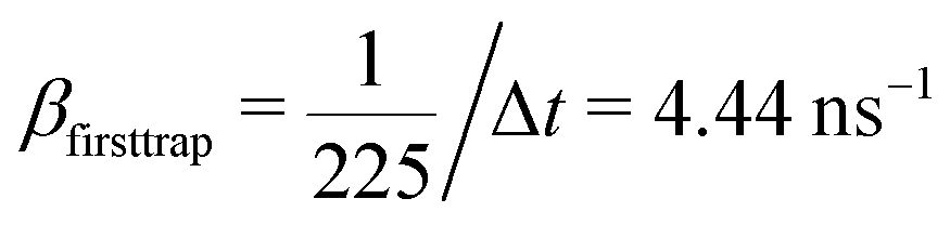 (the trapping rate is almost constant at short times). In order to account for the undercounting of trapping events at long times in our theoretical model, we slightly increase the trapping rate and set β = 7.5 ns−1. At long times, secondary trapping is quite likely since right after escape from a trap, a particle is more likely to come back than at earlier times.
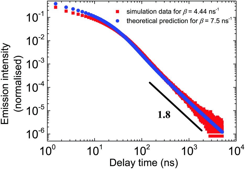
 .
.

 . Thus, we have established a link of the non-Markovian model (1)–(2) and the classical Markovian two-state equations.63
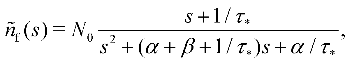


 that follows directly from eqn (3).
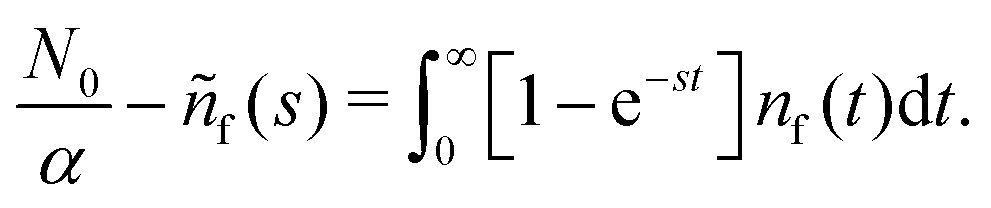
 . We put the latter expression in the identity and get