
 Open Access Article
 This Open Access Article is licensed under a
 Creative Commons Attribution 3.0 Unported Licence
Interface structures in ionic liquid crystals
Hendrik
Bartsch
 *ab,
Markus
Bier
abc and
Siegfried
Dietrich
ab
*ab,
Markus
Bier
abc and
Siegfried
Dietrich
ab
aMax Planck Institute for Intelligent Systems, Heisenbergstr. 3, 70569, Stuttgart, Germany. E-mail: hbartsch@is.mpg.de; bier@is.mpg.de
bInstitute of Theoretical Physics IV, University of Stuttgart, Pfaffenwaldring 57, 70569, Stuttgart, Germany
cUniversity of Applied Sciences Würzburg-Schweinfurt, Ignaz-Schön-Str. 11, 97421, Schweinfurt, Germany
First published on 30th April 2019
Abstract
Ionic liquid crystals (ILCs) are anisotropic mesogenic molecules which additionally carry charges. This combination gives rise to a complex interplay of the underlying (anisotropic) contributions to the pair interactions. It promises interesting and distinctive structural and orientational properties to arise in systems of ILCs, combining properties of liquid crystals and ionic liquids. While previous theoretical studies have focused on the phase behavior of ILCs and the structure of the respective bulk phases, in the present study we provide new results, obtained within density functional theory, concerning (planar) free interfaces between an isotropic liquid L and two types of smectic-A phases (SA or SAW). We discuss the structural and orientational properties of these interfaces in terms of the packing fraction profile η(r) and the orientational order parameter profile S2(r) concerning the tilt angle α between the (bulk) smectic layer normal and the interface normal. The asymptotic decay of η(r) and of S2(r) towards their values in the isotropic bulk is discussed, too.
1 Introduction
Ionic liquid crystals (ILCs) are pure ionic systems, solely composed of cations (+) and anions (−). Moreover, at least one of the ion species is characterized by a highly anisotropic molecular shape.1 This anisotropic shape is typically due to long alkyl-chains which are attached to charged moieties. Although the alkyl-chains exhibit a rather strong flexibility, due to microphase segregation of the charged parts and of the alkyl-chains, liquid-crystalline phases are indeed observable among ILCs.1–3 In the past decades various types of ILCs have been synthesized.1,3 Different combinations of, e.g., (charged) imidazolium rings and alkyl-chains allow one to tune not only the length of the ionic mesogenes but also the location of their charges, i.e., the intra-molecular charge distribution. Thereby one is able to promote distinctive properties of ILCs, for instance, a high thermal and high electrochemical stability, which might be beneficial for technological applications.1,3–6 (We note, that here the term “mesogene” refers to any kind of molecule which gives rise to the formation of mesophases, irrespective of the underlying microscopic mechanism. Accordingly, the aforementioned anisotropic molecules, which form mesophases via microphase segregation, are considered to be mesogenes.)A specific example of an ILC system, which has been studied, e.g., in ref. 7 and 8, is composed of cations with long alkyl-chains attached (1-dodecyl-3-methylimidazolium) and significantly smaller anions (iodide). For such an ILC system, one observes a liquid crystalline structure, in particular the smectic-A phase SA. (The SA phase is characterized by layers of particles which are well aligned with the layer normal and the layer spacing is of the size of the particle length.) The layer structure of the large cations leads to a locally increased concentration of anions in between the layers of cations.7 Thereby, the nanostructure of the cations gives rise to “pathways” for the anions, which increase the conductivity measurable in the direction parallel to the layers. Therefore this particular type of an ILC system is a promising candidate for technological applications, e.g., as electrolyte in dye-sensitized solar cells (DSSCs).7,9
While the complexity of the underlying interactions gives rise to these interesting properties of ILCs, it is at the same time very challenging to study these systems within theory or simulations. Previous theoretical studies10,11 of ILC systems have been able to reduce this complexity by considering a simplified description of ILC systems, which incorporates, however, the generic properties of ILCs. They rely on an effective one-species description in which one of the ion species (referred to as counterions) is not accounted for explicitly, but is incorporated as a continuous background, giving rise to the screening of the coions. On the contrary, the coions are modeled as ellipsoidal particles. Thus, the anisotropic molecular shape, which gives rise to the formation of mesophases, and the (screened) electrostatic interaction are both incorporated by this approach. Of course, this is a simplified representation of any realistic ionic liquid crystalline system. However, it allows one to study the interplay of the two key features, i.e., an anisotropic molecular shape and the presence of charges, which are omnipresent in ILC systems. Yet it should be noted, that ILC systems exhibiting a significant difference in size of the cations and of the anions (e.g., the aforementioned example of 1-dodecyl-3-methylimidazolium) might be candidates which come closest to the present theoretical representation of ILCs, as the size difference rationalizes in parts the idea of structureless point-like counterions.
As a first step, such a model allows one to study the phase behavior of ILC systems and thereby to gain insight about how molecular properties, e.g., the aspect-ratio or the charge distribution of the molecules, affect the phase behavior of such types of ILCs. A comprehensive understanding of the relation between the underlying molecular properties and the resulting phase behavior is inter alia, necessary for a systematic synthesis of ILCs, which should meet specific material properties. Furthermore, theoretical guidance is beneficial for finding and exploring novel materials properties which might occur in ILC systems. For instance, in ref. 11 a new smectic-A structure (SAW) has been observed, which exhibits an alternating layer structure. In between layers of elongated particles, which prefer to be oriented parallel to the layer normal, like in the ordinary SA phase, one observes secondary layers in which the particles prefer to be oriented perpendicular to it. Due to this alternating structure the layer spacing of this new SAW phase is significantly wider compared to the ordinary SA phase. The SAW structure is stabilized by charges which are located at the tips of the molecules. This shows in an exemplary way how the combination of liquid-crystalline behavior and electrostatics can lead to an interesting and novel phenomenology.
The aim of the present investigation is to extend the analysis by studying spatially inhomogeneous systems of ILCs. This is done by investigating how the structural and orientational properties of ILC systems are affected by the presence of a free interface between coexisting bulk states. Both smectic-A phases, SA and SAW, observed in ref. 11 can be in coexistence with the isotropic liquid phase L. This is of intrinsic interest, because it allows one to investigate interfaces which interpolate between a structured and orientationally ordered (i.e., smectic) phase and an isotropic, homogeneous, and thus structure-less, fluid phase. In particular, the transition in the structural and in the orientational order allows one to study the interplay of both properties while they build up at the interface. Although there are theoretical analyses12–18 concerning related types of free interfaces, in these studies the constituent particles are plain liquid crystals without any charges. On the other hand, there is a vast number of theoretical studies on ionic fluids. The thermodynamic behavior19–22 as well as the structure23–27 of these types of fluids, in which long-ranged Coulomb interactions are present, have been intensively studied. However, ionic systems are often analyzed assuming a simple geometry of the particles, such as a spherical shape of the particles like in the restricted primitive model.28–30 In this regard, the present study attempts to analyze the aforementioned type of interface between an isotropic and a smectic phase by accounting for an anisotropic particle shape combined with the presence of charges.
Moreover, different orientations between the interface normal and the smectic layer normal are possible. In this context, an interesting question addresses the equilibrium tilt angle between the interface and the smectic layer normal. This angle may provide insight into nucleation and growth phenomena which are affected by the dependence of the interfacial tension on the orientation of the considered structure.31,32
The present study is structured as follows: in Section 2 the model and the employed density functional theory approach are presented. Our results for the interfaces between the isotropic liquid L and the considered smectic-A phases SA or SAW are discussed in Section 3. Finally, in Section 4 we summarize the results and draw our conclusions.
2 Model and methods
This section presents in detail the molecular model of ILCs as employed here. In particular, we discuss the intermolecular pair potential, which can be applied to a wide range of ionic and liquid crystalline materials due to its flexibility provided by a large set of parameters.This model is studied by (classical) density functional theory (DFT), which will be applied to spatially inhomogeneous systems, in particular free interfaces formed between coexisting bulk phases. The methodological and technical details of the present DFT approach are described in Section 2.2.
2.1 Molecular model and pair potential
We consider a coarse-grained description of the ILC molecules as rigid prolate ellipsoids of length-to-breadth ratio L/R ≥ 1 (see Fig. 1). Thus, the orientation of a molecule is fully described by the direction ω(ϕ,ϑ) of its long axis, where ϕ and ϑ denote the azimuthal and polar angle, respectively.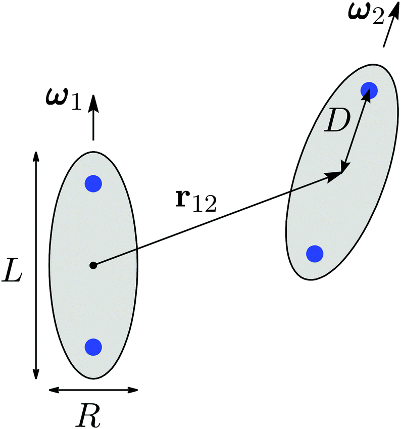 | ||
| Fig. 1 Cross-sectional view of two ILC molecules in the plane spanned by the orientations ωi, i = 1, 2, of their long axis. The particles are treated as rigid prolate ellipsoids, characterized by their length-to-breadth ratio L/R ≥ 1. Their orientations are fully described by the direction of their long axis ωi, i = 1, 2; r12 is the center-to-center distance vector. The charges of the ILC molecules (blue dots) are located on the long axis at a distance D from their geometrical center. The counterions are not modeled explicitly, but they are implicitly accounted for in terms of a background, giving rise to the screening of the charges of the ILC molecules. | ||
The two-body interaction potential consists of a hard core repulsive and an additional contribution UGB + Ues beyond the contact distance Rσ, the sum of which can be attractive or repulsive:
 | (1) |
![[r with combining circumflex]](https://www.rsc.org/images/entities/b_i_char_0072_0302.gif) 12,ω1,ω2) depends on the orientations of both particles and on the direction of the center-to-center distance vector, which is expressed by the unit vector 12 := r12/|r12|. In eqn (1), we have subdivided the contributions beyond the contact distance |r12| ≥ Rσ into two parts: UGB(r12,ω1,ω2) is the well-known Gay–Berne potential,33,34 which incorporates an attractive van der Waals-like interaction between molecules and which can be understood as a generalization of the Lennard-Jones pair potential between spherical particles to ellipsoidal particles:
12,ω1,ω2) depends on the orientations of both particles and on the direction of the center-to-center distance vector, which is expressed by the unit vector 12 := r12/|r12|. In eqn (1), we have subdivided the contributions beyond the contact distance |r12| ≥ Rσ into two parts: UGB(r12,ω1,ω2) is the well-known Gay–Berne potential,33,34 which incorporates an attractive van der Waals-like interaction between molecules and which can be understood as a generalization of the Lennard-Jones pair potential between spherical particles to ellipsoidal particles: | (2) |
 | (3) |
 | (4) |
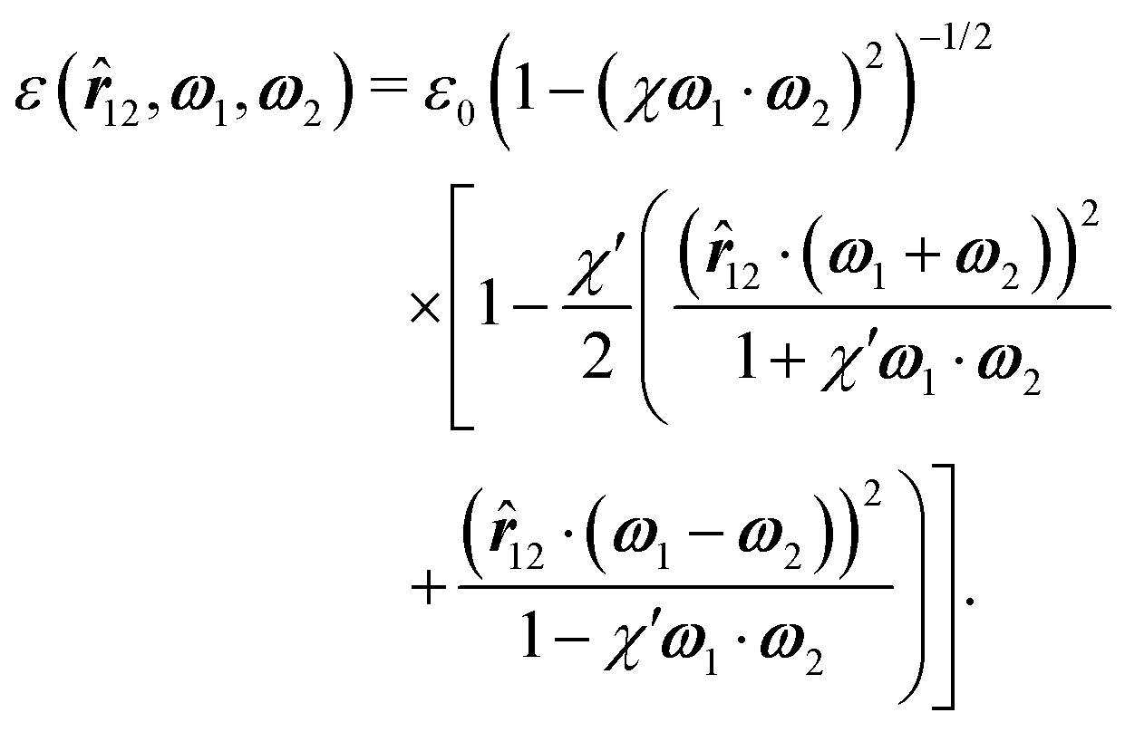
12,ω1,ω2) and the direction- and orientation-dependent interaction strength ε(12,ω1,ω2) are both parametrically dependent on the length-to-breadth ratio L/R via the auxiliary function χ = ((L/R)2 − 1)/((L/R)2 + 1). Additionally, ε(12,ω1,ω2) can be tuned via χ′ = ((εR/εL)1/2 − 1)/((εR/εL)1/2 + 1), where εR/εL is called the anisotropy parameter, defined in terms of the ratio of εR, which is the depth of the potential minimum for parallel particles positioned side by side (12·ω1 = 12·ω2 = 0), and εL, which is the depth of the potential minimum for parallel particles positioned end to end (12·ω1 = 12·ω2 = 1). The energy scale of the Gay–Berne pair interaction is set by ε0. Thus, the Gay–Berne pair potential has four independent free parameters: ε0, R, L/R, and εR/εL. Note that in the case of spherical particles, i.e., for L = R, the Gay–Berne pair potential (eqn (2)) reduces to the well-known isotropic Lennard-Jones pair potential if, additionally, the Gay–Berne anisotropy parameter equals unity, i.e., εR/εL = 1, because then σ(12,ω1,ω2) = 1 and ε(12,ω1,ω2) = ε0.
The second contribution Ues(r12,ω1,ω2) in eqn (1) is the electrostatic repulsion of ILC molecules. Within the scope of the present study, the counterions are not modeled explicitly. They will be considered to be much smaller in size than the ILC molecules such that they can be treated as a continuous background. On the level of linear response, this background gives rise to the screening of the pure Coulomb potential between two charged sites on a length scale given by the Debye screening length λD such, that the effective electrostatic interaction of the ILC molecules is given by
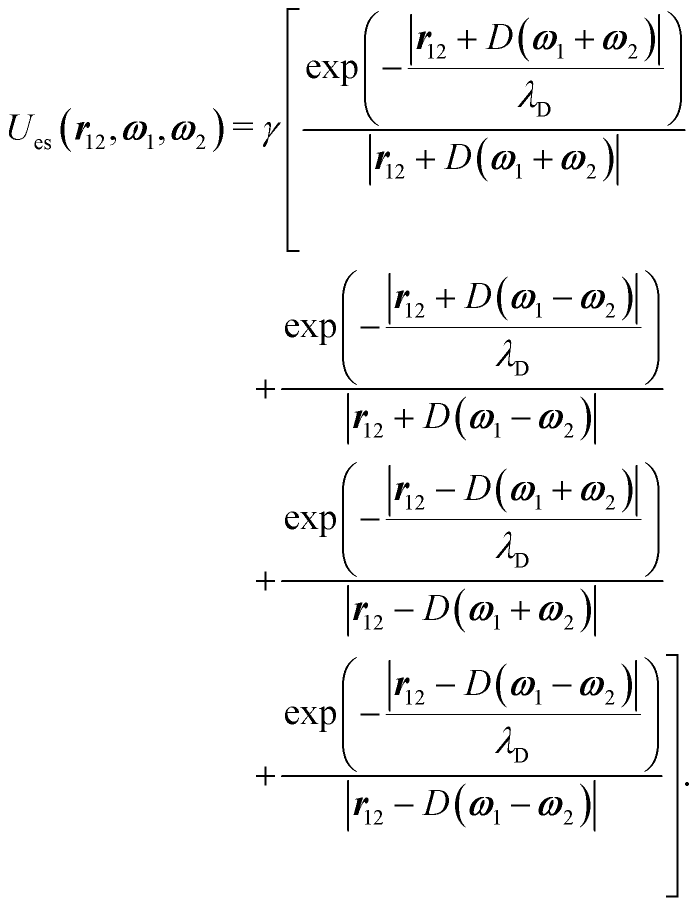 | (5) |
 | (6) |
In Fig. 2 we illustrate the full pair potential (eqn (1)) beyond the contact distance for certain choices of the parameters. The two top panels, (a) and (b), show the pure Gay–Berne potential (uncharged liquid crystals), which is predominantly attractive in the space outside the overlap volume (salmon-colored area). The shape of this overlap volume changes by varying the particle orientations as well as by changing the length-to-breadth ratio L/R. However, these dependences are not apparent from Fig. 2, because L/R = 4 and the particle orientations ωi are kept fixed for all panels. In panel (b) the anisotropy parameter εR/εL = 4 is chosen to be two times larger than for panel (a) (εR/εL = 2). Thus, the ratio of the well depth at the tails and at the sides is increased. The two bottom panels, (c) and (d), show the same choices for the Gay–Berne parameters as for panel (a), but the electrostatic repulsion of the charged groups on the molecules, illustrated by blue dots, is included (γ/(Rε0) = 0.25). In panel (c) the loci of the two charges of the particles coincide at their centers (i.e., D/R = 0) while in panel (d) they are located near the tips (D/R = 1.8). For both cases with charge, the effective interaction range is significantly increased compared with the uncharged case and is governed by the Debye screening length, chosen as λD/R = 5.
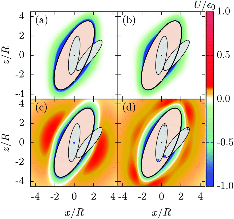 | ||
Fig. 2 Contour-plots of the pair potential U for |r12| ≥ Rσ in the x–z-plane for four cases of particles with fixed length-to-breadth ratio L/R = 4 and fixed orientations. In each panel the centers of both particles lie in the plane y = 0. In order to illustrate the orientations of the ellipsoids, they have been included in the plots at contact with relative direction 12 = ![[x with combining circumflex]](https://www.rsc.org/images/entities/b_i_char_0078_0302.gif) . The set of points at contact in the x–z-plane is illustrated by the black curve, and the centers of the particles are shown by small black dots. Panel (a): uncharged liquid crystal with εR/εL = 2. Panel (b): uncharged liquid crystal with εR/εL = 4. With this choice the anisotropy of the potential is increased slightly. Panel (c): ILC with εR/εL = 2, D/R = 0, λD/R = 5, γ/(Rε0) = 0.25. Panel (d): ILC with εR/εL = 2, D/R = 1.8, λD/R = 5, γ/(Rε0) = 0.25. In (c) and (d) the loci of the charges are indicated as blue dots. The salmon-colored area is the excluded volume for given orientations of the two particles. . The set of points at contact in the x–z-plane is illustrated by the black curve, and the centers of the particles are shown by small black dots. Panel (a): uncharged liquid crystal with εR/εL = 2. Panel (b): uncharged liquid crystal with εR/εL = 4. With this choice the anisotropy of the potential is increased slightly. Panel (c): ILC with εR/εL = 2, D/R = 0, λD/R = 5, γ/(Rε0) = 0.25. Panel (d): ILC with εR/εL = 2, D/R = 1.8, λD/R = 5, γ/(Rε0) = 0.25. In (c) and (d) the loci of the charges are indicated as blue dots. The salmon-colored area is the excluded volume for given orientations of the two particles. | ||
It is worth mentioning, that the present model cannot be considered as a quantitatively valid description of any realistic ionic liquid crystal system. A screened electrostatic pair interaction of the Yukawa form (eqn (5)) is the extreme case of the effective pair potential between ions in a (dilute) electrolyte at high temperatures. Nonetheless, for the purpose of the present theoretical study, which is concerned with the basic microscopic mechanisms and the generic molecular properties present in ILC systems, the employed model is appropriate as it incorporates the following key properties of ILCs: first, a sufficiently anisotropic shape (prolate) of the particles, i.e., they can be considered as (calamitic) mesogenes. In this context, an assessment of the bulk phase behavior, depending on the length-to-breadth ratio of the particles, is provided in ref. 11. In particular, the relevance of a sufficiently anisotropic shape (i.e., L/R > 2) for observing genuine smectic phases is discussed. Second, the ionic properties of ILCs are incorporated such that they reflect the main feature of ionic fluids, i.e., the effective interaction of the ionic compounds via a screened electrostatic pair interaction. Although the chosen functional form given by eqn (5) cannot be considered as a quantitatively reliable representation, it still accounts for the fact that the actual ion–ion pair interaction in an ionic fluid is indeed short-ranged, rather than long-ranged, as it is the case for the bare Coulomb interaction.
In conclusion, eqn (5) is characterized by an effective interaction strength γ/R (which will be numerically expressed as the relative interaction strength γ/(Rε0) compared to the interaction strength ε0 of the Gay–Berne potential), an effective interaction range λD, and an effective location D of the charge sites inside the coions. In order to represent specific ILC molecules by a particular set of parameters of the present model, one would tune the independent model parameters, i.e., L/R, εR/εL, γ/(Rε0), D/R, and λD/R such that the resulting total pair potential U(r12,ω1,ω2)/ε0 (compare eqn (1) and Fig. 2) resembles (qualitatively) the actual pair potential of the considered ILC molecules. In this regard, it is worth mentioning that in principle comparisons of our effective theory with particle simulations can be made, related to the study by Saielli et al.,35 who performed molecular dynamics (MD) simulations for a mixture of (ellipsoidal) Gay–Berne and (spherical) Lennard-Jones particles. Additionally, both species carry charges and therefore resemble cations and anions, respectively. Our ad hoc pair potential (eqn (1)) of the coions can be compared with the effective interaction, which can be determined as the logarithm of the particle–particle distribution function of the elongated cations in the MD simulations.
We note, that the choices L/R = 4 and εR/εL = 2, which are used throughout our analysis, are comparable to those used in previous studies (see, e.g., ref. 10, 11, 35 and 36) for similar kinds of particles. While these values of the Gay–Berne parameters give rise to the formation of smectic phases, the occurrence of nematic phases is typically observed for much larger values of L/R and εR/εL.37
2.2 Density functional theory
The degrees of freedom of the particles (compare Section 2.1) are fully described by the positions r of their centers and the orientations ω of their long axes. Thus, within density functional theory, an appropriate variational grand potential functional βΩ[ρ] of position- and orientation-dependent number density profiles ρ(r,ω) has to be found; the equilibrium density profile minimizes the functional. The grand potential functional for uniaxial particles, in the absence of external fields, can generically be expressed as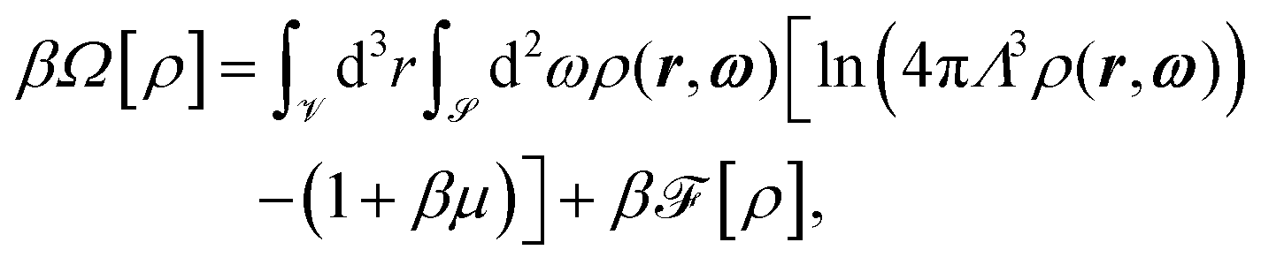 | (7) |
![[scr V, script letter V]](https://www.rsc.org/images/entities/char_e149.gif) and
and ![[scr S, script letter S]](https://www.rsc.org/images/entities/char_e532.gif) denote the system volume and the full solid angle, respectively. The first term in eqn (7) is the purely entropic free energy contribution of non-interacting uniaxial particles, where β = 1/(kBT) denotes the inverse thermal energy, μ the chemical potential, and Λ the thermal de Broglie wavelength.
denote the system volume and the full solid angle, respectively. The first term in eqn (7) is the purely entropic free energy contribution of non-interacting uniaxial particles, where β = 1/(kBT) denotes the inverse thermal energy, μ the chemical potential, and Λ the thermal de Broglie wavelength.
The last term is the excess free energy β![[scr F, script letter F]](https://www.rsc.org/images/entities/char_e141.gif) [ρ] in units of kBT, which incorporates the effects of the inter-particle interactions. Minimizing eqn (7) leads to the Euler–Lagrange equation, which implicitly determines the equilibrium density profile ρ(r,ω):
[ρ] in units of kBT, which incorporates the effects of the inter-particle interactions. Minimizing eqn (7) leads to the Euler–Lagrange equation, which implicitly determines the equilibrium density profile ρ(r,ω):
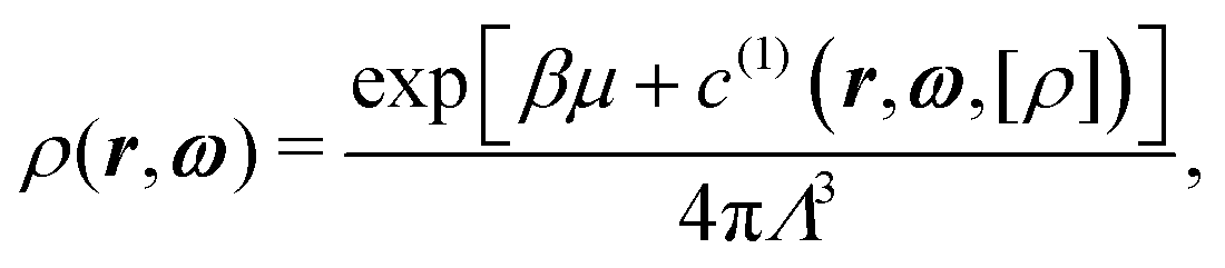 | (8) |
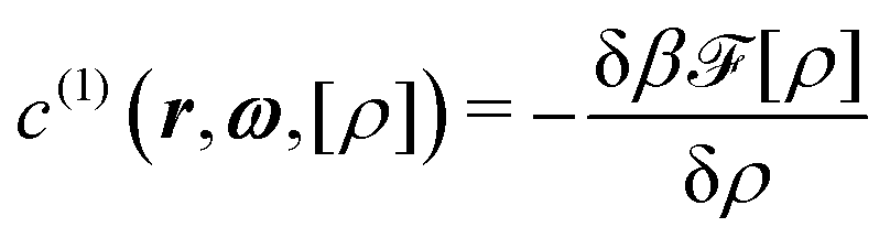 | (9) |
[ρ].
The excess free energy functional is the characterizing quantity of the underlying many-body problem. However, in general it is not known exactly so that one has to adopt appropriate approximations of it. Following the approach of our previous study11 concerning the bulk phase behavior of ILCs, in the spirit of ref. 38 a weighted density expression for β[ρ] is considered:
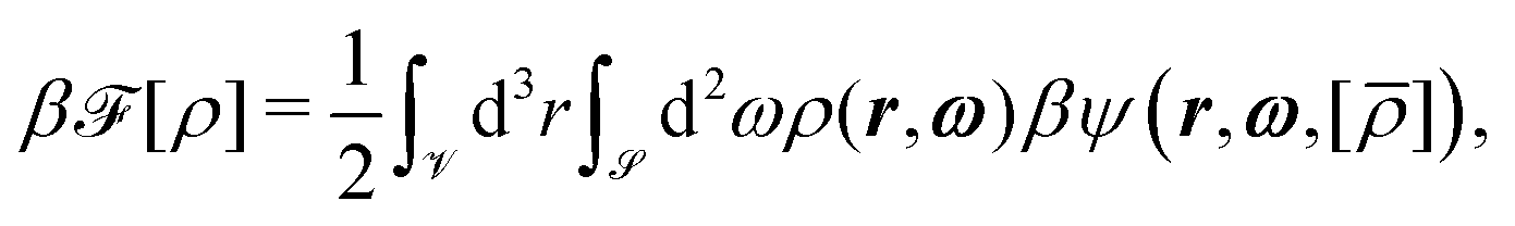 | (10) |
![[small rho, Greek, macron]](https://www.rsc.org/images/entities/i_char_e0d1.gif) ]) denotes the effective one-particle potential. It is a functional of the so-called projected density (r,ω):
]) denotes the effective one-particle potential. It is a functional of the so-called projected density (r,ω):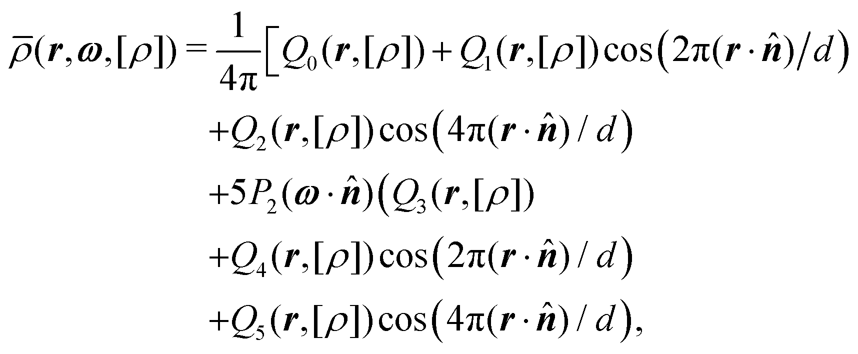 | (11) |
(r,ω) represents an expansion of the density profile ρ(r,ω) in terms of a second-order Fourier, and a second-order Legendre series, respectively. Thus, the coefficients Qi(r) are the corresponding expansion coefficients, which will be defined below. It is worth mentioning, that although the projected density (r,ω) might take negative values, this does not imply an unphysical behavior as the actual density ρ(r,ω) is determined from the Euler–Lagrange equation (i.e., eqn (8)) and thus is strictly positive. The following three types of bulk phases can be studied within this particular framework:11 first, isotropic liquids with Q0 = const0 and Qi = 0 for i > 0. Second, nematic liquids with Qi = consti, if i = 0, 3, and Qi = 0 otherwise. Third, smectic-A phases with Qi = consti for i ∈ {0,…,5}. While for isotropic and nematic liquids the system is translationally invariant in all spatial directions, in the case of smectic-A phases the system is periodic in the direction of the smectic layer normal ![[n with combining circumflex]](https://www.rsc.org/images/entities/b_i_char_006e_0302.gif) with periodicity d, which is a multiple of the smectic layer spacing. For smectic-A phases the director is parallel to the smectic layer normal and therefore the occurrence of rotationally symmetric distributions of the orientations ω around , incorporated by the dependence on ω· in eqn (11), are plausible. We note that odd Fourier-modes in the projected density (r,ω) vanish for bulk smectic-A phases, if the coordinate system is chosen such that the origin is located at the center of one of the smectic layers due to the mirror symmetry of smectic layers around their center. This is a direct consequence of the underlying point symmetry of the particles considered here (see Fig. 1). Considering additional terms, corresponding to the odd modes in the second-order Fourier expansion of the density ρ(r,ω), would only give rise to a shift of the location of the bulk smectic layers. Although for systems with interfaces the odd modes in general do not vanish, here we neglect these contributions completely. The implications of additionally considering the odd terms (up to second order) are discussed in Appendix A. Both approaches are weighted-density-like approximations of the exact free energy functional. A priori, it is not obvious which one leads to better results, because considering more terms of the Fourier series leads only to a more accurate representation of ρ(r,ω) by the projected density (r,ω). However, this does not imply that the resulting free energy functional β[] is closer to its exact form, because independent of the choice for (r,ω) it relies on the Parsons–Lee approach for its reference part and on the so-called modified mean-field approximation for the excess part (see below). Nevertheless, our approach of considering in eqn (11) only the even modes up to second order captures the three types of bulk phases L, N, as well as SA, SAW, which are relevant for the present study in the same way as the full second-order Fourier expansion.
with periodicity d, which is a multiple of the smectic layer spacing. For smectic-A phases the director is parallel to the smectic layer normal and therefore the occurrence of rotationally symmetric distributions of the orientations ω around , incorporated by the dependence on ω· in eqn (11), are plausible. We note that odd Fourier-modes in the projected density (r,ω) vanish for bulk smectic-A phases, if the coordinate system is chosen such that the origin is located at the center of one of the smectic layers due to the mirror symmetry of smectic layers around their center. This is a direct consequence of the underlying point symmetry of the particles considered here (see Fig. 1). Considering additional terms, corresponding to the odd modes in the second-order Fourier expansion of the density ρ(r,ω), would only give rise to a shift of the location of the bulk smectic layers. Although for systems with interfaces the odd modes in general do not vanish, here we neglect these contributions completely. The implications of additionally considering the odd terms (up to second order) are discussed in Appendix A. Both approaches are weighted-density-like approximations of the exact free energy functional. A priori, it is not obvious which one leads to better results, because considering more terms of the Fourier series leads only to a more accurate representation of ρ(r,ω) by the projected density (r,ω). However, this does not imply that the resulting free energy functional β[] is closer to its exact form, because independent of the choice for (r,ω) it relies on the Parsons–Lee approach for its reference part and on the so-called modified mean-field approximation for the excess part (see below). Nevertheless, our approach of considering in eqn (11) only the even modes up to second order captures the three types of bulk phases L, N, as well as SA, SAW, which are relevant for the present study in the same way as the full second-order Fourier expansion.
The effective one-particle potential βψ(r,ω) consists of two contributions. The first one incorporates the hard-core interactions via the well-studied Parsons–Lee functional,39,40
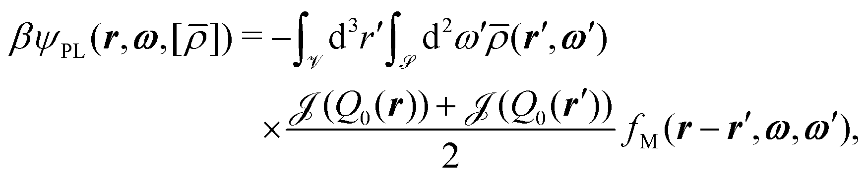 | (12) |
![[scr J, script letter J]](https://www.rsc.org/images/entities/char_e529.gif) (Q0) modifies the corresponding original Onsager free energy functional (i.e., the second-order virial approximation) such that the Carnahan–Starling equation of state40 is reproduced for spheres, i.e., for L = R:42, 43
(Q0) modifies the corresponding original Onsager free energy functional (i.e., the second-order virial approximation) such that the Carnahan–Starling equation of state40 is reproduced for spheres, i.e., for L = R:42, 43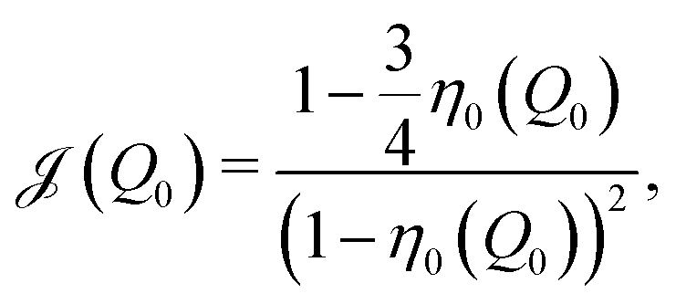 | (13) |
(Q0) by Q0.
The second contribution to the effective one-particle potential βψ[] takes into account the interactions beyond the contact distance (see the case |r12| ≥ Rσ in eqn (1)) within the modified mean-field approximation,44 which is a variant of the extended random phase approximation (ERPA):45
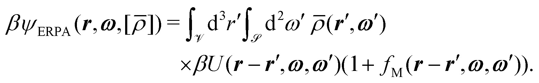 | (14) |
The present study is devoted to the analysis of free interfaces which are formed between coexisting bulk phases. In particular, the planar interfaces between the isotropic liquid L and the two different types of smectic-A phases (SA or SAW, see Section 3) will be considered, for which the interface normal is expected to be parallel to the z-direction (see Fig. 3). Due to the isotropy of the liquid phase L, the direction of the smectic layer normal
| (α) := sin(α) + cos(α)ẑ | (15) |
= ẑ points into the z-direction, like the interface normal, while for α = π/2 it points into the x-direction and thus it is perpendicular to the interface normal. The interfacial systems considered here are translationally invariant in the y-direction and show a periodic structure in the x-direction with a periodicity dx = d/sin(α) (compare Fig. 3) where d is a multiple of the smectic layer spacing (we note that the value of d is determined by the corresponding bulk density distribution which minimizes the grand potential functional, i.e., maximizes the bulk pressure (see Section 2.2.2 in ref. 11). It turns out that, for the SAW phase d equals the smectic layer spacing, while for the SA phase it equals two times the layer spacing, because for the SA phase one obtains bulk solutions ρ(0)(r,ω) with Q1 = Q4 = 0, (see, cf., eqn (11), (16) and (17)). Thus the periodicity d along the layer normal is twice the smectic layer spacing, i.e., the distance between neighboring layers). For α = 0, dx diverges and the system is translationally invariant in the x-direction, too.
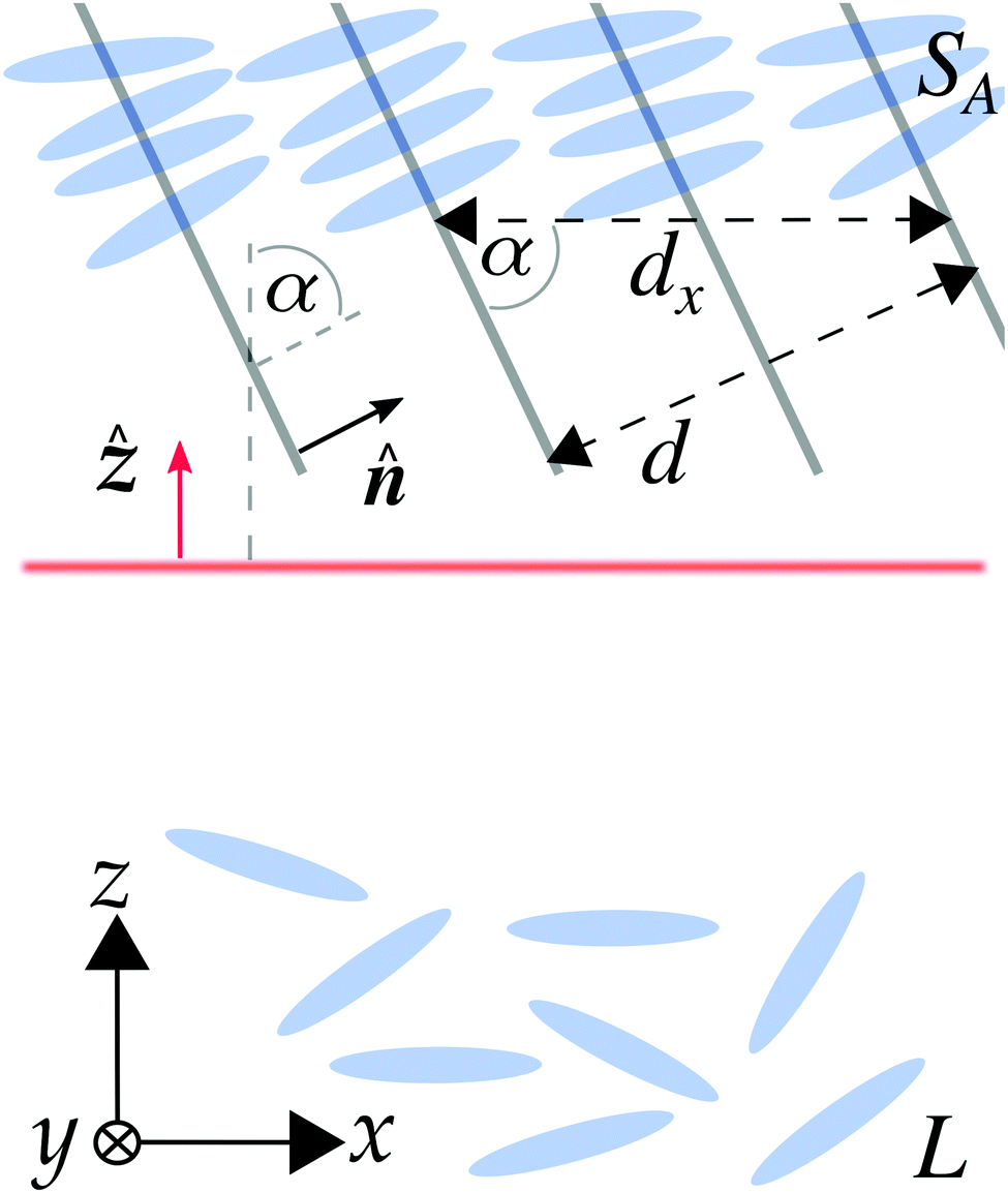 | ||
| Fig. 3 Sketch of the interface structure under consideration. Consider a planar interface, illustrated by the horizontal red line, between the isotropic bulk liquid L, imposed as the boundary condition at z → −∞, and the smectic-A phase SA (or SAW), imposed as the boundary condition at z → +∞. Thus, the interface normal (red vertical arrow) points into the z-direction. At the top, the tails of four layers of particles of the (ordinary) SA phase are visible, which are well aligned with the smectic layer normal := sin(α) + cos(α)ẑ. In the bulk SA phase, the system is periodic in the direction of the smectic layer normal with periodicity d which is a multiple of the smectic layer spacing. For the SA phase d turns out to be two times the distance between neighboring smectic layers (see Section 2.2 below eqn (15)). Thus, for a given tilt angle α between the interface normal and the smectic layer normal , the system is periodic in x-direction with periodicity dx = d/sin(α). Note that the interface structure is translationally invariant in the y-direction for all angles 0 ≤ α ≤ π/2. For α = 0 the system exhibits in addition translational invariance in the x-direction. | ||
As mentioned above, the coefficients Qi(r) in eqn (11) arise from expanding ρ(r,ω) in a second-order Legendre- and Fourier-series:11
 | (16) |
 | (17) |
 | (18) |
![[scr T, script letter T]](https://www.rsc.org/images/entities/char_e533.gif) (r − r′) is a cut-off function which defines the integration domain
(r − r′) is a cut-off function which defines the integration domain 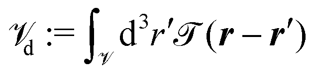 around position r. For 0 < α ≤ π/2 the considered interfaces between the isotropic liquid L and the smectic-A phases SA or SAW exhibit periodic structures in the x-direction with periodicity dx = d/sin(α). Here, d is a slice of length dx in x-direction with a vanishing extension in z-direction centered at position r, i.e., (r − r′) = Θ(dx/2 − |x − x′|)δ(z − z′) where Θ(x) and δ(x) are the Heaviside step function and the Dirac delta function, respectively. The index d of the integration domain d indicates that d corresponds to a region which is specified by the periodicity d. Due to the translational invariance in y-direction the extension of the integration domain d can be chosen arbitrarily in the y-direction. Due to the periodicity of ρ(r,ω) in the x-direction, this choice of the integration domain d leads to coefficients Qi(z) (eqn (16)) which depend only on z, i.e., on the coordinate parallel to the interface normal.
For 0 < α ≤ π/2 one could also consider an integration domain which has a non-vanishing extent in z-direction. However, such a choice has at least two disadvantages: first, unlike dx, which corresponds to the periodicity of the system in x-direction, for 0 < α ≤ π/2 there is no obvious choice for the extent of d parallel to the interface normal. Additionally, there is no unique choice for the geometrical shape of the integration domains; besides using a rectangular form, one could also use any other (two-dimensional) geometrical object as integration domain d. In this sense the slice of length dx perpendicular to the interface normal is a simple but also consistent choice. Second, this choice renders the evaluation numerically less demanding, because it requires only a one-dimensional integration (exploiting the translational invariance in y-direction), instead of evaluating a two-dimensional integral. We note, that an infinite extent of the integration domain parallel to the interface normal leads to coefficients Qi which are independent of the position r and therefore cannot be used to obtain interface profiles.
If α = 0, i.e., the smectic layer normal = ẑ is parallel to the interface normal, dx diverges and the system is translationally invariant in x- and y-direction. In this case, the integration domain d has an extent of length d in z-direction, i.e., (r − r′) = Θ(d/2 − |z − z′|) with arbitrary extent in the lateral dimensions x and y. As before, the coefficients Qi(z) depend only on the z-coordinate. It is worth mentioning, that for all tilt angles 0 ≤ α ≤ π/2 the correct (constant) bulk values of the coefficients Qi are recovered, although for 0 < α < π/2 the orientation of the integration domain d (recall that d is a slice of width dx in x-direction for all α ∈ (0,π/2]) changes with respect to the direction of the smectic layer normal (α). However, because the integration domain covers a full period dx in x-direction, it gives the same values for the coefficients Qi in the bulk phases, as for evaluating the coefficients Qi with an integration domain parallel to the smectic layer normal , which is the case for α = 0 and π/2.
Finally, the one-particle direct correlation function c(1)(r,ω,[ρ]) can be derived by considering eqn (9) which leads to the following (modified) expression for c(1)(r,ω,[ρ]) (compare eqn (21) in ref. 11):
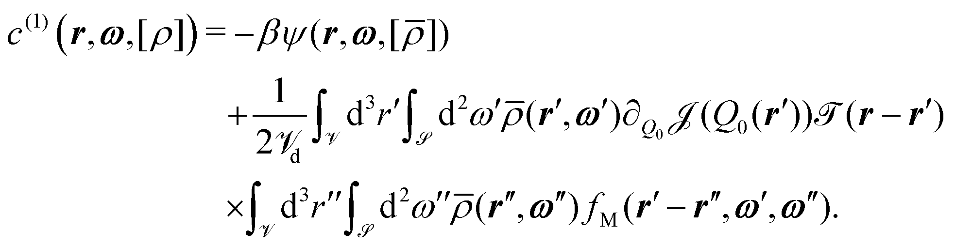 | (19) |
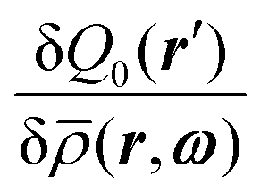 has been replaced by
  . This replacement, i.e., the equation
 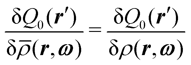 , is valid exactly only for bulk phases. In general, these two functional derivatives are related via
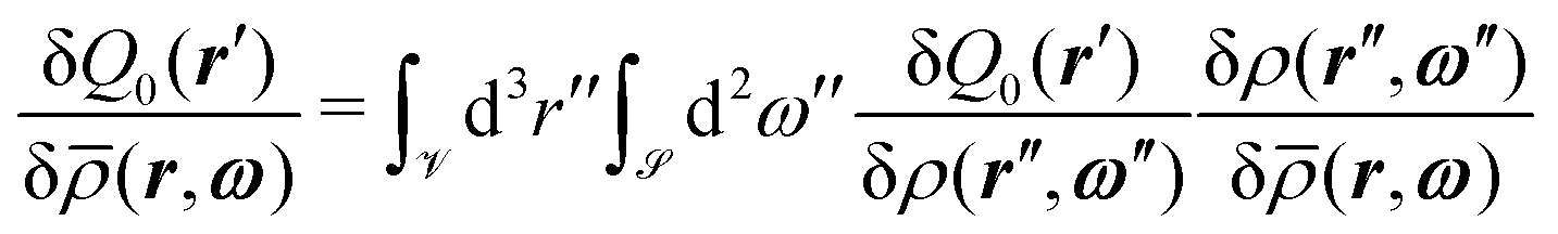 , which, however, cannot be calculated analytically. Determining
  requires the functional derivative of the Euler–Lagrange equation (i.e., eqn (8)) which would in turn produce terms containing
  . Nevertheless, the derivation of eqn (19) (following from eqn (21) in ref. 11) incorporates a modification of the exact one-particle direct correlation function such that the density profile ρ(r,ω) is replaced by the projected density (r,ω). In this respect, replacing
  by
by 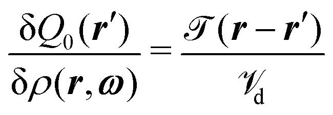 (which follows from eqn (16)–(18)) is consistent with our approach, as it also implies an exchange of ρ(r,ω) and (r,ω). Moreover, the exchange renders the correct bulk limit of the interface profile ρ(r,ω) at the boundaries, i.e., z → ±∞.
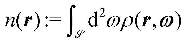
Eqn (8) has been solved numerically (utilizing a Picard scheme with retardation) by using eqn (19) as well as the (constant) bulk values of the coefficients Qi,L = Qi(z → −∞) in the isotropic liquid phase L and Qi,S = Qi(z → ∞) in the smectic-A phase (SA or SAW)) at coexistence (T,μ) = (Tcoex,μcoex). The structural properties and the orientational order at the free interface are analyzed in terms of the interface profiles of the packing fraction
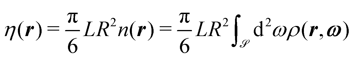 | (20) |
 , and in terms of the orientational order parameter
 | (21) |
2.3 Gibbs dividing surface
The position zη of the interface is determined by the density profile ρ(r,ω) for which we have adopted the notion of the Gibbs dividing surface:41 | (22) |
| zη = −hη(0)/(η0,SA − η0,L), | (23) |
| zS2 = −hS2(0)/(S20,SA − S20,L), | (24) |
Note, that instead of using the mean packing fraction η0 or the mean orientational order parameter S20 in eqn (22), for determining the interface positions, in principle, one could also use the profiles η(r) and S2(r) directly. However, the disadvantage of this latter approach is that in the smectic-A bulk phase SA (or SAW) the profiles η(r) and S2(r) are still functions of the position r (via the projection r· onto the layer normal ). Typically, this prevents the use of the latter generalized eqn (23) and (24) for determining zη and zS2. Instead, one has to solve eqn (22) numerically, which requires many iterations depending on the desired accuracy.
Nevertheless, in the particular case α = π/2 the interface normal and the smectic layer normal are perpendicular. Due to the translational invariance of the smectic phases perpendicular to their layer normal, here the density profile η(z → ∞) and the orientational order parameter profile S2(z → ∞) do not depend on z for z → ∞ in the smectic bulk, but they depend only on the x-coordinate. Thus, for α = π/2 one can define interface contours ![[z with combining tilde]](https://www.rsc.org/images/entities/i_char_007a_0303.gif) η(x) and S2(x), analogously to zη and zS2:
η(x) and S2(x), analogously to zη and zS2:
 | (25) |
2.4 Interfacial tension
The interfacial tension Γ is a measure of the excess amount of work needed to form an interface between coexisting bulk phases.41 Accordingly, it can be calculated by determining the increase in the grand potential βΩ[ρ] of the interface system in excess of the bulk grand potential βΩ0 := −βp which is given by the bulk pressure p (see eqn (26) in ref. 11) times the system volume : | (26) |
3 Results
In this section we present results for free interfaces formed between the isotropic liquid L and the smectic-A phase SA or SAW. The discussion focuses on two kinds of ionic liquid crystals (ILCs) which are described by the pair interaction potential U(r12,ω1,ω2) (eqn (1)), introduced in Section 2.1: first, ILCs with charges in the center, i.e., D = 0 (see Fig. 1 and eqn (5)), and second, ILCs with charges at the tips, i.e., D/R = 1.8. In particular the structural and orientational properties of the interface are discussed in terms of the packing fraction profile η(r) and the orientational order parameter profile S2(r) for various relative orientations between the interface normal and the smectic layer normal, i.e., for different tilt angles α (see Fig. 3). All results presented here have been obtained via the density functional approach described in Section 2.2.3.1 Interface normal parallel to the smectic layer normal (α = 0)
First, we consider the case that the interface normal is parallel to the normal of the smectic layers, i.e., α = 0 (see Fig. 3). Both point into the z-direction and due to translational invariance in the x- and y-directions, the packing fraction η(z) and the orientational order parameter S2(z) are functions solely of the spatial coordinate z. For the case of an ionic liquid crystal with L/R = 4, εR/εL = 2, γ/(Rε0) = 0.045, λD/R = 5, and D = 0, i.e., the charges are localized in the center of the molecule, the bulk phase behavior is shown in the T*–η0-phase diagrams of Fig. 4(a) where T* = kT/ε0 and η0 = Q0LR2π/6 are the reduced temperature and the mean packing fraction, respectively. Within the considered temperature range T* ∈ [0.9,1.65] solely a first-order phase transition from the isotropic liquid phase L to the ordinary smectic-A phase SA occurs. The SA phase is characterized by a layer structure with a smectic layer spacing d/R ≈ 4.3, which is comparable to the particle length L/R = 4. Within the smectic layers the particles are well aligned with the smectic layer normal. The blue lines in Fig. 4(a) correspond to L–SA-coexistence and the light blue area in between the coexistence lines represents the two-phase region.
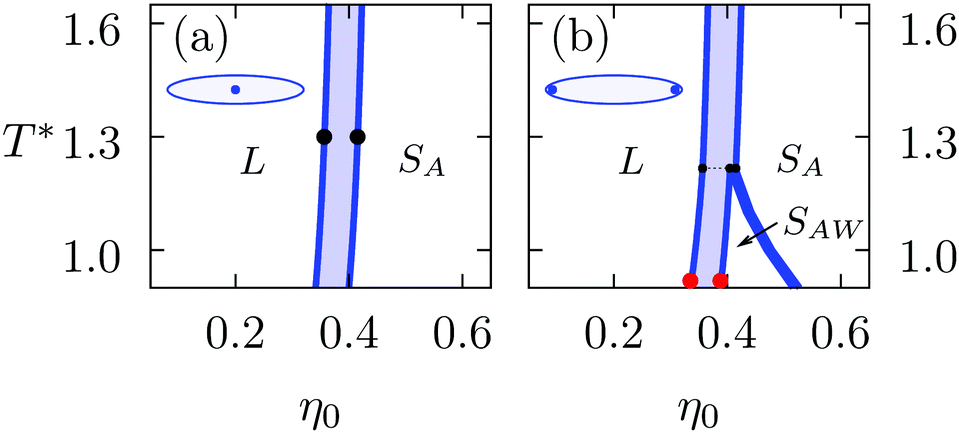 | ||
Fig. 4 Bulk phase diagrams for (a) ionic liquid crystals with L/R = 4, εR/εL = 2, γ/(Rε0) = 0.045, λD/R = 5, and D = 0 and (b) with L/R = 4, εR/εL = 2, γ/(Rε0) = 0.045, λD/R = 5, and D/R = 1.8. For D = 0, i.e., the charges being concentrated in the center of the molecules, solely a first-order phase transition from the isotropic liquid phase L to the ordinary smectic-A phase SA occurs at sufficiently high mean packing fractions η0. The ordinary smectic-A phase SA is characterized by a layer structure with smectic layer spacing d/R ≈ 4.3 ≳ L/R = 4 comparable with the particle length L. The particles in the layers are well aligned with the layer normal . In panel (b), i.e., for D/R = 1.8 (the charges being located at the tips of the molecules), another smectic-A structure, referred to as the SAW phase can be observed at low reduced temperatures T*. The SAW phase exhibits an alternating structure, consisting of primary layers of particles being parallel to the layer normal and secondary layers in which the particles prefer to be perpendicular to it. This leads to an increased layer spacing d/R ≥ 7.5. The black dotted line in panel (b) marks the triple point at T* ≈ 1.23 for which the isotropic liquid L, the ordinary smectic-A phase SA, and the SAW phase are in three-phase-coexistence. A detailed description of the structural properties of the smectic-A phases SA and SAW, including illustrations of their microstructure, are provided in ref. 11. The black dots (•) in panel (a), respectively the red dots ( ) in (b), mark the coexisting bulk states at the reduced temperature T* = 1.3, respectively 0.9, imposed as boundary conditions for the free interfaces shown in Fig. 5 and 7–9. ) in (b), mark the coexisting bulk states at the reduced temperature T* = 1.3, respectively 0.9, imposed as boundary conditions for the free interfaces shown in Fig. 5 and 7–9. | ||
The L–SA-interface is shown in Fig. 5 for T* = 1.3. In the phase diagram in Fig. 4(a) the corresponding two coexisting bulk states are marked by black dots (•). Panels (a) and (b) show the packing fraction profile η(z) along the interface normal and the orientational order parameter profile S2(x), respectively. The black dashed vertical line in panel (a) marks the position zη of the Gibbs dividing surface, which is defined by eqn (23). Correspondingly, the black dashed vertical line in panel (b) marks the position zS2 (eqn (24)). Apparently, the two interface positions zη and zS2, which are related to the interfacial transition in the structure and in the orientational order, respectively, differ from each other. In Fig. 6, these differences zη − zS2 are plotted as function of the reduced temperature T* for three different kinds of liquid-crystalline systems. The violet curve corresponds to ILCs with all charges concentrated in the molecular centers, i.e., D = 0, while the green curve shows data points for D/R = 1.8. The blue curve corresponds to a system of ordinary (uncharged) liquid crystals (OLCs) described by L/R = 4, εR/εL = 2, and γ/(Rε0) = 0. The phase diagram for OLCs is not shown here; it is presented in Fig. 4(a) of ref. 11. Within the considered temperature ranges, in all three cases the differences are at most as large as the length of the particle diameter R, which in turn is much smaller than the smectic layer spacing d/R ≈ 4.3 which is comparable to the particle length L, because the particles within the smectic layers are well aligned with the z-direction, indicated by S2(z) > 0.8 in the centers of the smectic layers. Thus, the small size of the differences shows that in these cases the transition in the orientational order and in the fluid structure go along with each other. As soon as the smectic layer structure dies out, the orientational order vanishes as well.
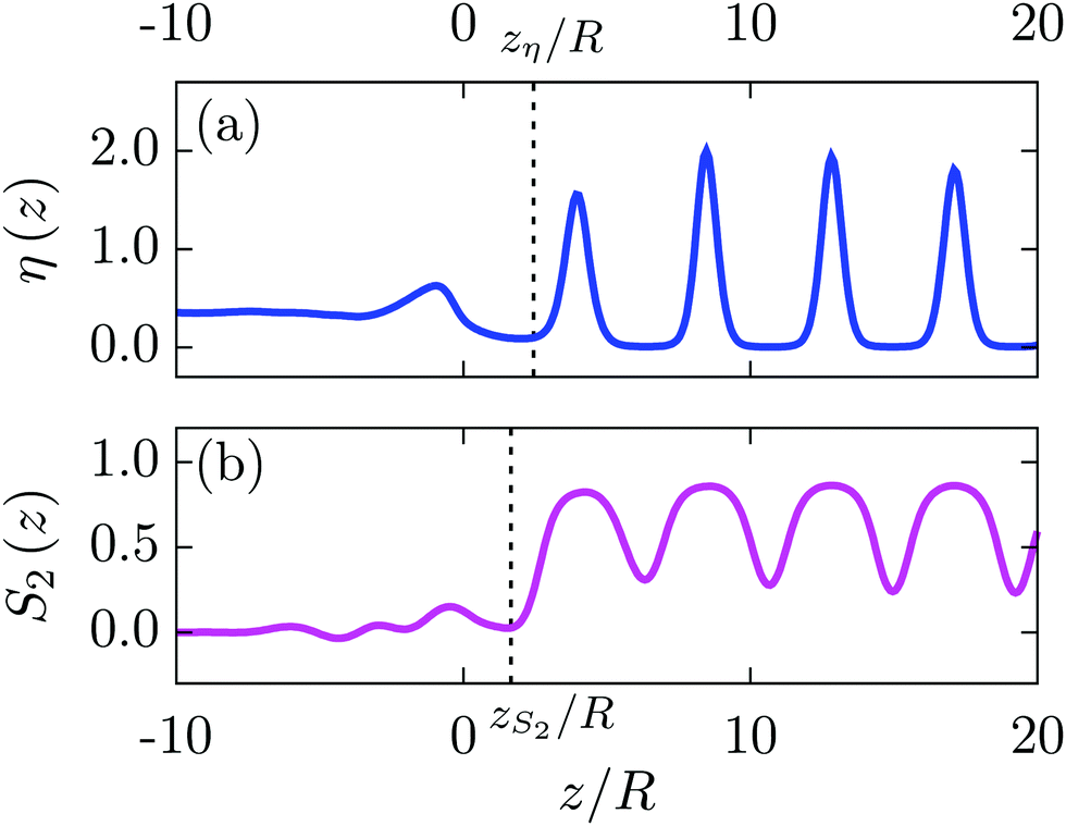 | ||
| Fig. 5 The L–SA-interface profile of the packing fraction η(z), panel (a), and the orientational order parameter S2(z), panel (b), are shown for an ionic liquid crystal with L/R = 4, εR/εL = 2, γ/(Rε0) = 0.045, λD/R = 5, and D = 0, i.e., the charges are concentrated in the center of the molecules. The free interface between the isotropic liquid L (imposed as boundary condition for z → −∞) and the ordinary smectic-A phase SA (i.e., z → ∞) is considered for the reduced temperature T* = 1.3. The corresponding coexisting bulk states are marked by the black dots (•) in the phase diagram in Fig. 4(a). The tilt angle is α = 0, i.e., the smectic layer normal = ẑ is parallel to the interface normal (see Fig. 3). For z/R > 0 the last layers of the SA phase are visible, in which the particles are still well aligned with the z-axis, indicated by large values of the orientational order parameter S2(z/R) > 0.8 within these layers. For z/R < 0 the layer structure of the density dies out rapidly and the orientational order vanishes as well. Ultimately, the isotropic bulk limit will be approached for z → −∞. However, already for z/R < −10 the profiles have de facto reached their bulk limits in the isotropic liquid L. The black dashed lines refer to the interface positions zη and zS2, respectively, calculated viaeqn (23) and (24). The difference (zη − zS2)/R ≈ 2.45 − 1.66 = 0.79 between the two interface positions is considerably smaller than the smectic layer spacing d/R ≈ 4.28 ≳ L/R = 4. Therefore the orientational order of the SA phase vanishes within the last smectic layer while approaching the isotropic liquid L. | ||
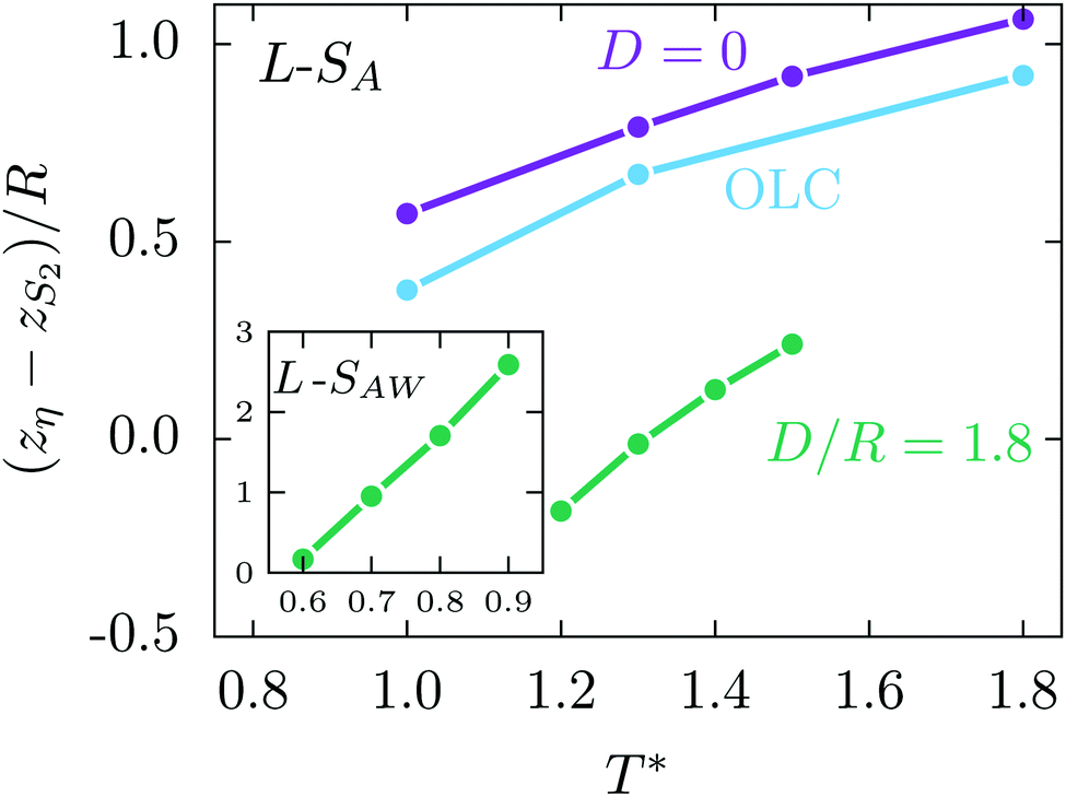 | ||
| Fig. 6 The difference (zη − zS2)/R between the Gibbs dividing surface position zη (eqn (23)), and the surface position zS2 (eqn (24)), which corresponds to the transition of the orientational order at the interface, are shown for three cases. First, an ordinary (uncharged) liquid crystal (OLC; blue curve); second, ILCs with charges in their center, i.e., D = 0 (violet curve); and, third, ILCs with charges at the tips, i.e., D/R = 1.8 (green curve). Here, the smectic layer normal = ẑ is parallel to the interface normal, i.e., α = 0. In all cases studied, the differences (zη − zS2)/R are smaller than the smectic layer spacing d ≳ L, which for the SA phase is comparable to the particle length L/R = 4. Thus, the loss of orientational order occurs within the last smectic layer before approaching the isotropic liquid L. The inset shows data for the L–SAW-interface, which are accessible for D/R = 1.8 at sufficiently low temperatures T*. Although the difference (zη − zS2)/R is enlarged for 0.7 < T* ≤ 0.9, it is still considerably smaller than the layer spacing d/R ≈ 7.5 and decreases rapidly upon decreasing the temperature T*. Hence, for α = 0, the orientational order of the smectic-A phase, either SA or SAW, vanishes directly with the disappearance of the layer structure at the interface. | ||
While for ILCs with charges in their center, within the considered temperature range, only L–SA-coexistence is observable (see Fig. 4(a)). For ILCs with the charges at the tips, such as in the case L/R = 4, εR/εL = 2, γ/(Rε0) = 0.045, λD/R = 5, and D/R = 1.8, the bulk phase behavior changes significantly at low temperatures, i.e., for T* < 1.23. The bulk phase diagram in Fig. 4(b) shows that in this case the distinct smectic-A phase SAW occurs for intermediate mean packing fraction η0. The SAW phase is characterized by an alternating layer structure of smectic layers with a majority of particles being oriented parallel to the smectic layer normal and a minority of particles localized in secondary layers which prefer orientations perpendicular to the smectic layer normal. Due to this alternating layer structure the smectic layer spacing d/R ≈ 7.5 is increased for the SAW phase. A detailed discussion of the structural and orientational properties of this new and peculiar smectic-A phase, in particular concerning the bulk density and the orientational order parameters profiles, is given in ref. 11.
In Fig. 7 the L–SAW-interface profiles η(z) and S2(z) are shown for α = 0 and T* = 0.9. In the phase diagram in Fig. 4(b) the corresponding coexisting bulk states are marked by red dots ( ). On the right hand side of Fig. 7 the alternating layer structure of the bulk SAW phase is evident. In the main layers the majority of the particles (η(z) > 2) has orientations parallel to the z-axis (S2(z) > 0.8) and in the secondary layers, formed by less of them (η(z) ≈ 0.6), the particles prefer orientations perpendicular to the z-axis (S2(z) < 0). For the L–SAW-interface the difference (zη − zS2)/R ≈ 2.6 of the two interface positions is increased compared to the L–SA-interface (see Fig. 6), because the smectic layer spacing d/R ≥ 7.5 in the SAW phase is enlarged, too. As before, the orientational order directly vanishes with the disappearance of the layer structure. Furthermore, the inset in Fig. 6 shows that (zη − zS2)/R decreases upon lowering the temperature. Thus the difference zη − zS2 becomes smaller relative to the layer spacing d, such that the direct vanishing of the orientational order associated with the disappearance of the layer structure is observable for the whole temperature range considered here.
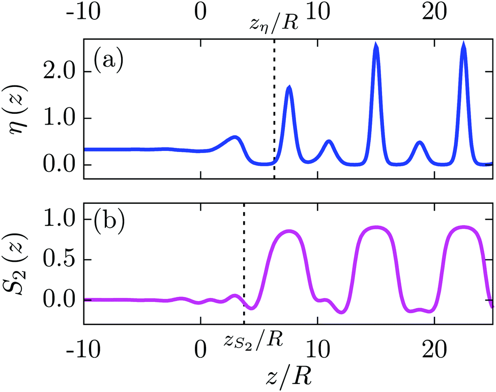 | ||
Fig. 7 For α = 0, the L–SAW-interface profiles η(z) and S2(z) are shown for ILCs with charges at the tips (L/R = 4, εR/εL = 2, γ/(Rε0) = 0.045, λD/R = 5, and D/R = 1.8) at the reduced temperature T* = 0.9 (see the red dots ( ) in Fig. 4(b)). For z → −∞ the isotropic liquid bulk L is approached whereas for z → ∞ the SAW bulk is attained. The difference (zη − zS2)/R ≈ 6.31 − 3.72 = 2.59 between the two interface positions is larger than the one of the L–SA-interface (compare Fig. 5 and 6) but it is still smaller than the smectic layer spacing d/R = 7.5. Therefore the orientational order of the SAW phase also vanishes within the range of the last smectic layer at the interface. ) in Fig. 4(b)). For z → −∞ the isotropic liquid bulk L is approached whereas for z → ∞ the SAW bulk is attained. The difference (zη − zS2)/R ≈ 6.31 − 3.72 = 2.59 between the two interface positions is larger than the one of the L–SA-interface (compare Fig. 5 and 6) but it is still smaller than the smectic layer spacing d/R = 7.5. Therefore the orientational order of the SAW phase also vanishes within the range of the last smectic layer at the interface. | ||
3.2 Interface normal perpendicular to the smectic layer normal (α = π/2)
For α = π/2 the interface normal and the smectic layer normal are perpendicular to each other. The smectic layer normal points into the x-direction and the interface normal into the z-direction (see Fig. 3). The associated L–SA-interface at T* = 1.3 for an ILC system with the charges concentrated at the center, described by the parameter set L/R = 4, εR/εL = 2, γ/(Rε0) = 0.045, λD/R = 5, and D = 0, is shown in Fig. 8. The corresponding bulk phases are given by the state points marked by black dots (•) in the phase diagram in Fig. 4(a). Panel (a) shows the packing fraction η(x,z) and (b) the orientational order parameter S2(x,z). The red areas at the top of Fig. 8(a) show the tails of four smectic layers of the SA phase located at x/R = ±d/(2R) ≈ ±2.14 and x/R = ±3d/(2R) ≈ ±6.42 where d/R ≈ 4.28 is the smectic layer spacing. The particles are well aligned with the smectic layer normal = indicated by large values of the orientational order parameter S2(x,z) > 0.8 in the layers.
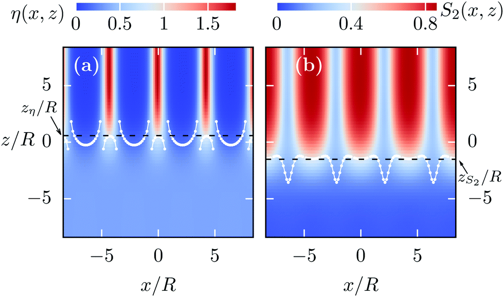 | ||
| Fig. 8 The L–SA-interface profiles η(x,z), panel (a), and S2(x,z), panel (b), are shown for T* = 1.3 (see the black dots (•) in Fig. 4(a)) and α = π/2. Accordingly, the smectic layer normal = and the interface normal (parallel to the z-axis) are perpendicular. Here, ILCs with charges at the center are considered, described by the parameter set L/R = 4, εR/εL = 2, γ/(Rε0) = 0.045, λD/R = 5, and D = 0. For z → −∞ the isotropic bulk liquid L and for z → ∞ the bulk of the SA phase is approached. The decaying red stripes at the upper part of these plots show the tails of the smectic layers located at x/R ≈ 0, ±d/R, ±2d/R where d/R ≈ 4.28 is the smectic layer spacing. The black dashed lines mark the interface positions zη and zS2 calculated viaeqn (23) and (24), while the white dotted lines mark the interface contours η(x) and S2(x) calculated viaeqn (25). The difference (zη − zS2)/R ≈ 0.58 − (−1.51) = 2.09 is larger than the particle diameter R, which is the relevant geometrical property of the particles at this interface, because for α = π/2 the particles in the SA layers are well aligned with the x-axis and therefore they are oriented perpendicular to the direction of the interface normal. The orientational order of the smectic-A phase persists up to a few particle diameters into the liquid phase, unlike the case α = 0, in which the disappearance of the layer structure causes a direct vanishing of the orientational order within the last layer (see Fig. 5–7). | ||
The black dashed lines in Fig. 8 show the interface positions zη and zS2 calculated from eqn (23) and (24), while the white dotted lines show the interface contours η(x) and S2(x) obtained from eqn (25). The contour lines η(x) and S2(x) at the centers of the tails of the smectic layers, e.g., at x/R ≈ 2.14, are very close to zη and zS2, respectively. This suggests that the two distinct definitions of the interface positions, i.e., using either eqn (23) and (24) or eqn (25), are consistent with each other, because the majority of the particles in the smectic phase are located close to the centers of the smectic layers. In Fig. 8(a) the packing fraction interface contour η(x) exhibits discontinuities for lateral positions ![[x with combining breve]](https://www.rsc.org/images/entities/i_char_0078_0306.gif) ; at which the smectic bulk packing fraction ηSA() := η(, z → ∞) takes the same value ηL = η(, z → −∞) as in the isotropic liquid L, i.e., ηSA() = ηL. Thus, the numerical calculation of the Gibbs dividing surface viaeqn (25) leads to a divergence due to the vanishing denominator. This can be considered as an artifact, which, however, occurs only at the particular lateral positions . Nevertheless, the benefit of considering η(x) and S2(x) as interface positions is their dependence on the lateral coordinate x. In particular, for the case of the L–SAW-interface it is necessary to consider η(x) and S2(x) in order to study the interface at the main layers and at the secondary layers separately (see below).
; at which the smectic bulk packing fraction ηSA() := η(, z → ∞) takes the same value ηL = η(, z → −∞) as in the isotropic liquid L, i.e., ηSA() = ηL. Thus, the numerical calculation of the Gibbs dividing surface viaeqn (25) leads to a divergence due to the vanishing denominator. This can be considered as an artifact, which, however, occurs only at the particular lateral positions . Nevertheless, the benefit of considering η(x) and S2(x) as interface positions is their dependence on the lateral coordinate x. In particular, for the case of the L–SAW-interface it is necessary to consider η(x) and S2(x) in order to study the interface at the main layers and at the secondary layers separately (see below).
Interestingly, if the layer normal and the interface normal are perpendicular, one observes a significant difference (zη − zS2)/R ≈ 0.72 − (−1.76) = 2.48 between the interface position zη, corresponding to the structural transition, and zS2 corresponding to the transition in the orientational order between the coexisting phases. Hence, the alignment of the particles with the x-axis persists a few particle diameters deeper into the liquid phase L than the layer structure of the SA phase is maintained – unlike in the case α = 0, i.e., in which the smectic layer normal is parallel to the interface normal, for which the orientational order directly vanishes when the smectic layers disappear (see Section 3.1). We note, that the vanishing of the orientational order significantly after (upon approaching the interface from the orientational ordered phase) the structural transition associated with the density profile, has already been observed previously18 in the case of the interface between an isotropic liquid and a plastic-triangular crystal (PTC).
For the type of ILCs with the charges at the tips, at low temperatures the new wide smectic-A phase SAW can be observed (see Fig. 4(b)). It is characterized by an alternating structure of layers in which the particles are predominantly parallel to the layer normal = (like in the SA phase) and layers of particles which are preferentially perpendicular to the layer normal. The free interface formed between the isotropic liquid L and the SAW phase for T* = 0.9 and α = π/2 is shown in Fig. 9. The red regions in Fig. 9(a) show the layers of particles (at x = 0 and x/R ≈ ±d/R = ±7.5) being parallel to the layer normal, while in between (at x/R ≈ ±d/(2R) = ±3.75) in light blue color the secondary layers are visible. The dark blue color at x/R ≈ ±d/(2R) = ±3.75 in panel (b) shows that the orientational order parameter S2(x,z) is negative at the location of the secondary layers, because there the particles are preferentially perpendicular to the layer normal. The interface at the parallel layers behaves very much like the L–SA interface, as can be inferred from the (white) interface contours η(x/R = 0, ±7.5)/R ≈ 0.81 and S2(x/R = 0, ±7.5)/R ≈ −1.83 which show that the orientational ordering of the SAW phase persists into the liquid phase L for a few particle diameters. This is also apparent from the interface positions zη/R ≈ 1.0 and zS2/R ≈ −2.3, depicted by the black dashed lines in Fig. 9. Conversely, at lateral positions x/R ≈ d/(2R) = ±3.75 associated with the centers of the intermediate layers, it turns out that the orientational order undergoes the transition before the layer structure vanishes if one approaches the interface from the SAW side (S2(x/R = ±3.75)/R ≈ 3.39 and η(x/R = ±3.75)/R ≈ −0.34; in order to guide the eye the magenta dots ( ) in Fig. 9 mark these positions). This behavior is opposite to the above one and is presumably related to the fact, that the secondary layers consist of particles being preferentially perpendicular to the layer normal; unlike the particles in the main layers of the SAW phase or the particles in the SA layers, these particles do not align with the layer normal = . Instead they are avoiding an orientation parallel to it. While the transition across the L–SA interface – from alignment with the layer normal towards an isotropic orientational distribution – results in an increase of the effective particle diameter in the y- and z-direction, for the secondary SAW layers the effective diameter is decreased from the SAW phase towards the isotropic liquid L. In Fig. 9 there are discontinuities in the (white) interface contour lines η(x) and S2(x), as in Fig. 8. These discontinuities occur at lateral positions at which the packing fraction η(, z → ±∞) or the orientational order parameter S2(, z → ±∞) take the same value in the isotropic bulk, i.e., for z → −∞, as in the SAW bulk, i.e., for z → ∞.
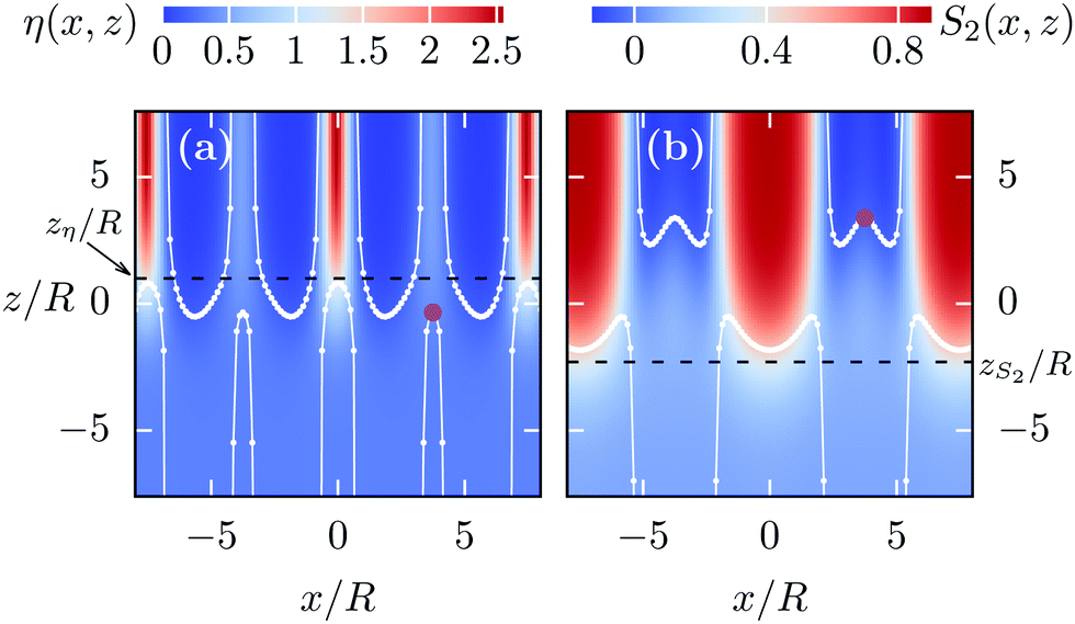 | ||
Fig. 9 The interface profiles η(x,z) and S2(x,z) for T* = 0.9 and α = π/2. Here the L–SAW interface (see the red dots ( ) in Fig. 4(b)) for an ILC with the charges at the tips (L/R = 4, εR/εL = 2, γ/(Rε0) = 0.045, λD/R = 5, and D/R = 1.8) is considered. The thin red areas in panel (a) for lateral positions x/R = 0, ±d/R = ±7.5 show the tails of the smectic layers where the particles prefer an orientation parallel to the smectic layer normal = . This is indicated by the large value of S2(x,z) > 0.8 within these layers. In panel (a) the secondary layers of the SAW phase are shown as light blue areas in panel (a) located at x/R = ±d/(2R) = ±3.75. There, the orientational order parameter S2(x,z), shown in panel (b), is negative. The black dashed lines mark the interface positions zη and zS2 calculated viaeqn (23) and (24), while the white dotted lines mark the interface contours η(x) and S2(x), which have been calculated viaeqn (25). The differences (zη − zS2)/R ≈ 1.0 − (−2.3) = 3.3, respectively (η(x) − S2(x))/R ≈ 0.81 − (−1.83) = 2.64 at the lateral positions x/R ≈ 0, ±7.5, exhibit a persisting orientational order for the main layers, similar to the findings for the L–SA interface (compare Fig. 8). Interestingly, at the secondary layers (x/R = ±d/(2R) = ±3.75) the orientational order vanishes ahead of the disappearance of the layer structure, i.e., S2(x/R = ±3.75)/R ≈ 3.39 > −0.34 ≈ η(x/R = ±3.75)/R. In order to guide the eye, the magenta dots ( ) in Fig. 4(b)) for an ILC with the charges at the tips (L/R = 4, εR/εL = 2, γ/(Rε0) = 0.045, λD/R = 5, and D/R = 1.8) is considered. The thin red areas in panel (a) for lateral positions x/R = 0, ±d/R = ±7.5 show the tails of the smectic layers where the particles prefer an orientation parallel to the smectic layer normal = . This is indicated by the large value of S2(x,z) > 0.8 within these layers. In panel (a) the secondary layers of the SAW phase are shown as light blue areas in panel (a) located at x/R = ±d/(2R) = ±3.75. There, the orientational order parameter S2(x,z), shown in panel (b), is negative. The black dashed lines mark the interface positions zη and zS2 calculated viaeqn (23) and (24), while the white dotted lines mark the interface contours η(x) and S2(x), which have been calculated viaeqn (25). The differences (zη − zS2)/R ≈ 1.0 − (−2.3) = 3.3, respectively (η(x) − S2(x))/R ≈ 0.81 − (−1.83) = 2.64 at the lateral positions x/R ≈ 0, ±7.5, exhibit a persisting orientational order for the main layers, similar to the findings for the L–SA interface (compare Fig. 8). Interestingly, at the secondary layers (x/R = ±d/(2R) = ±3.75) the orientational order vanishes ahead of the disappearance of the layer structure, i.e., S2(x/R = ±3.75)/R ≈ 3.39 > −0.34 ≈ η(x/R = ±3.75)/R. In order to guide the eye, the magenta dots ( ) mark the positions (x/R, η/R) ≈ (3.75, −0.34) and (x/R, S2/R) ≈ (3.75, 3.39). ) mark the positions (x/R, η/R) ≈ (3.75, −0.34) and (x/R, S2/R) ≈ (3.75, 3.39). | ||
3.3 Asymptotic behavior
In this section we discuss how the interface profiles of the packing fraction η(r) and the orientational order parameter S2(r) attain their respective values ηL and S2,L in the bulk liquid L. In Fig. 10 the asymptotic behavior is discussed in terms of ln|η(x,z) − ηL| and ln|S2(x,z) − S2,L| for α = π/2 and T* = 10, considering ILCs with charges in the center, i.e., D = 0 (panels (a) and (b)), and with charges at the tips, i.e., D/R = 1.8 (panels (c) and (d)). In order to elucidate the view angle on these 3-dimensional logarithmic plots, the interface profiles η(x,z) and S2(x,z) are shown in addition as contour plots (see Fig. 8) at the base of the respective plot. | ||
| Fig. 10 L–SA interface profiles of η(x,z) and S2(x,z) for T* = 10 and α = π/2. Accordingly, the smectic layer normal = and the interface normal (parallel to the z-axis) are perpendicular. Panels (a) and (b) show the logarithmic deviations ln|η(x,z) − ηL| and ln|S2(x,z) − S2,L| of the packing fraction and the orientational order parameter from their bulk values in the isotropic liquid L for an ILC with the charges concentrated at the center of the molecule, i.e., for D = 0. Panels (c) and (d) show ln|η(x,z) −ηL| and ln|S2(x,z) − S2,L| for an ILC with the charges at the tips, i.e., for D/R = 1.8. Note that on the base of each plot the interface profiles η(x,z) and S2(x,z) are shown in order to elucidate the viewing angle on the interface. The local height of the manifold above the base corresponds to the given color code. Interestingly, for D = 0 the periodic structure is still apparent even far away from the L–SA-interface, i.e., z/R < −20, unlike the case D/R = 1.8, for which the profiles are rather flat in lateral direction x. This can be related to the strong localization of charges at the centers of the smectic layers for D = 0, pronouncing the periodic structure, while for D/R = 1.8 the charge sites are spread and less localized along the x-direction. | ||
Interestingly, while for D = 0 the periodic structure of the profiles η(x,z) and S2(x,z) in x-direction is clearly apparent also in the decays ln|η(x,z) − ηL| and ln|S2(x,z) − S2,L| far away from the L–SA-interface (z/R < −20 in Fig. 10(a) and (b)), for D/R = 1.8 (panels (c) and (d)) the decays vary only little as function of x. This distinct behavior can be a signature of the respective molecular charge distributions, because if the charges are localized at the centers of the molecules, due to the layer structure in the SA phase the charges are also localized at the centers of the smectic layers, while for D/R = 1.8 the charges are less localized along the lateral direction x. Close to the interface (z/R > −20) the structure is very similar in both cases and, as will be discussed later, it is the hard-core repulsion which is the dominant contribution here.
Turning the view parallel to the x-axis, one obtains projected representations of the logarithmic plots in Fig. 10, which are shown in Fig. 11 keeping the order of panels as in Fig. 10. Hence, Fig. 11(a) and (b) correspond to the case D = 0 presenting ln|η(x,z) − ηL| and ln|S2(x,z) − S2,L|, respectively. Similarly, Fig. 11(c) and (d) show the case D/R = 1.8. In both cases, at large distances, i.e., z/R < −20, the decay of the density profiles is dominated by the electrostatic contribution Ues to the total interaction potential U (see Fig. 11(a) and (c)). Accordingly, the decay of the envelope is determined by the Debye screening length λD/R = 5, highlighted by the orange lines in Fig. 11. It is worth mentioning that a DFT study46 of the asymptotic behavior of the liquid–vapor interface has yielded, unlike the present findings, a decay length lb larger than the Debye screening length λD for a hard sphere system with additional Yukawa interaction. While in the present study the Yukawa potential is purely repulsive, in ref. 46 using an attractive Yukawa potential is indispensable, because a sufficiently strong attraction is needed for liquid–vapor coexistence to occur.
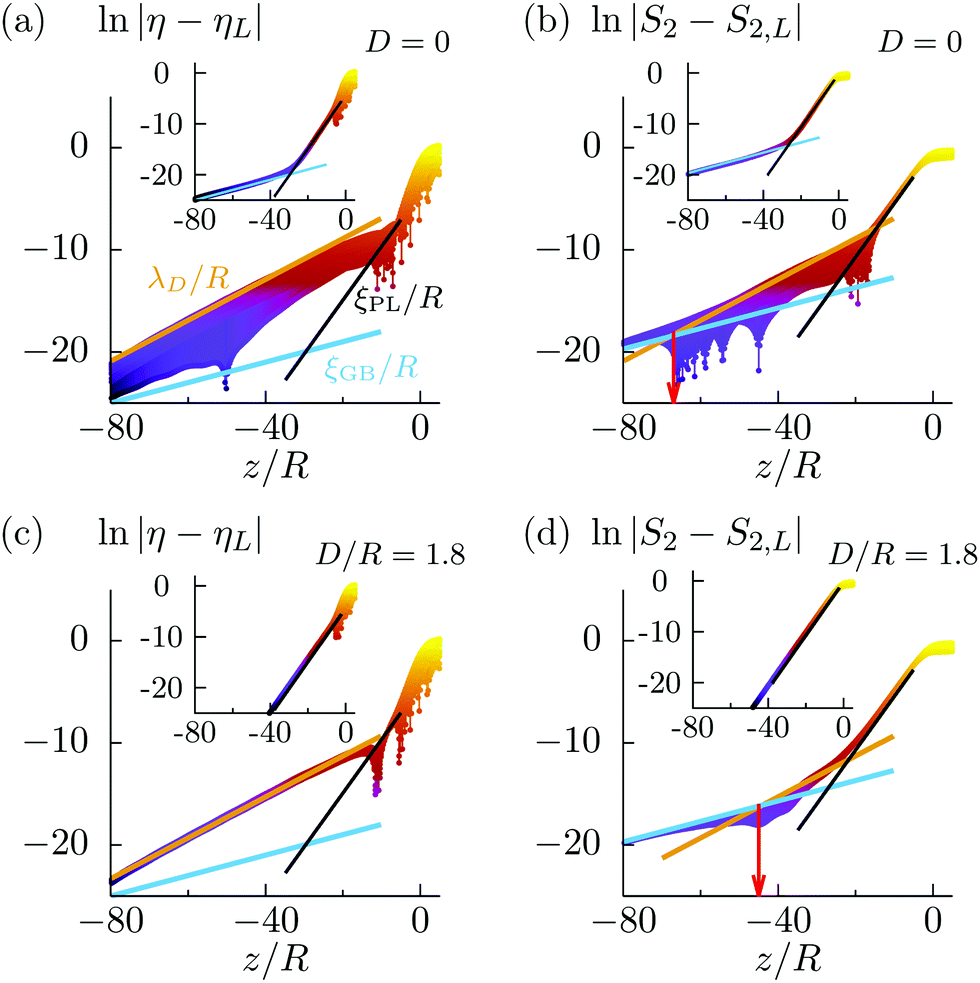 | ||
| Fig. 11 The same quantities as shown in Fig. 10. Panels (a) and (b) correspond to the case D = 0 presenting ln|η(x,z) − ηL| and ln|S2(x,z) − S2,L|, respectively, whereas panels (c) and (d) correspond to the case D/R = 1.8. However, here the direction of view is parallel to the x-axis so that the manifold from Fig. 10 is projected onto the plane spanned by the vertical axis and the z axis. Away from the interface, i.e., for z/R < −20, the decay length for ln|η(x,z) −ηL| can be identified as the Debye screening length λD/R = 5 for both cases (a) D = 0 and (c) D/R = 1.8. From the inset in panel (a), which shows ln|η(x,z) − ηL| for the corresponding (uncharged) ordinary liquid crystal with L/R = 4 and εR/εL = 2, it is apparent that the contributions due to the Gay–Berne potential (the asymptotics of which is indicated by the blue line) and due to the hard-core interaction (the asymptotics of which is depicted by the black line) are much weaker than the (screened) electrostatic contribution and do not play a role within the range of ln|η(x,z) − ηL| considered here. (In order to guide the eye, the blue and black lines are also shown in the main plots. Apparently, in (a) and (c) the blue and black lines are far below the respective profiles.) However, for ln|S2(x,z) − S2,L|, i.e., for panels (b) and (d), one observes crossovers – indicated by the intersection of the orange and blue lines at z/R ≈ −67 in (b) and z/R ≈ −45 in (d) (compare the red arrows in the respective plots) – from the electrostatic regime towards the decay governed by the Gay–Berne contribution with decay length ξGB/R ≈10. Such crossovers occur within the considered range z/R ∈ [−80,0], because for the orientational order parameter the amplitude of the decay, due to the Gay–Berne interaction, is larger than for the packing fraction (compare the intersections of the blue lines with the ordinates in panels (a) and (b)). Due to the hard-core interaction, for z/R > −20 the decay length ξPL/R ≈ 1.9 (Parsons–Lee, black lines) is visible for the ordinary liquid crystal in the insets of (a) and (b) as well as for ln|S2(x,z) − S2,L| of the two considered ILCs. (Due to the small amplitudes of the hard-core contributions to ln|η(x,z) − ηL|, for the ILC considered here, this decay has not been observed.) In order to confirm, that the decay length ξPL/R ≈ 1.9 is indeed due to the hard-core interaction, the insets of the panels (c) and (d) show ln|η(x,z) − ηL| and ln|S2(x,z) − S2,L| of the pure hard-core system (βψ := βψPL). Interestingly, ln|η(x,z) − ηL| and ln|S2(x,z) − S2,L| behave very similarly close to the interface, i.e., z/R > −10, for all three kinds of systems studied here. This suggests that the structure and the orientational properties close to the interface are governed by the hard-core interaction which enters into the present DFT approach (see Sections 2.1 and 2.2). | ||
Interestingly, the asymptotic behavior of the orientational order parameter at far distances, i.e., for z/R < −60, differs from the electrostatic decay and another regime (highlighted by blue lines in Fig. 11) with a larger decay length ξGB/R ≈ 10 sets in. This longer-ranged decay is due to the Gay–Berne interaction UGB which is verified by calculating the interface profile for an ordinary liquid crystal (OLC) without charges (compare the insets of panels (a) and (b) of Fig. 11). For the OLC, at far distances, i.e., z/R < −30, the same large decay length ξGB/R ≈ 10 is observed. However, the amplitudes of the decay of the packing fraction and of the orientational order parameter differ significantly. (The blue line in panel (a) intersects the ordinate at ln|η − ηL| ≈ −25, whereas the blue line in (b) intersects the ordinate at ln|S2 − S2,L| ≈ −20.) For D = 0, it turns out that for the orientational order parameter the crossover from the electrostatic decay towards the Gay–Berne decay occurs at z/R ≈ −67 (this position is marked by the red arrow in Fig. 11(b)), whereas for the case D/R = 1.8 the crossover occurs at z/R ≈ −45 (see the red arrow in Fig. 11(d)). Ultimately, the larger Gay–Berne decay length ξGB/R ≈ 10 will also become apparent in the decay profile of the packing fraction. However, due to the smaller amplitude of the Gay–Berne decay of the density compared with the decay of the orientational order parameter (compare the insets in Fig. 11(a) and (b)), in the present case the crossover occurs further away from the interface (in Fig. 11(a) the intersection of the orange line and the blue line is located at z/R ≈ −121 (not visible) and in Fig. 11(c) at z/R ≈ −97 (also not visible)). However, at very far distances z/R < −80, the magnitudes ln|η − ηL| ≲ −25 are very small and cannot be resolved numerically. For this reason, in Fig. 11(a) and (c) crossovers from the electrostatic regime to the Gay–Berne regime are not shown.
We note that, although the Gay–Berne potential UGB decays algebraically ∝(r12/R)−6 (see eqn (2)), here the Gay–Berne decay is exponential, because solving the Euler–Lagrange equation in eqn (8) requires the evaluation of the ERPA contribution βψERPA of the effective one particle potential βψ (see eqn (14) and (19)). The numerical calculation of this integral (which extends over the whole volume of the system) requires a truncation in terms of a cut-off distance of the integral which leads to an exponential decay of this contribution, instead of a power law decay ∝(z/R)−3,46–48 as it is expected for the full Gay–Berne potential UGB. (The exponent 3 arises because the asymptotic behavior of an interfacial density profile, generated by long-ranged forces, varies proportional to the corresponding (total) potential, which acts on a test particle at a distance z from the interface and which is due to the pair interaction between the particles in one of the two coexisting phases (which are separated by the considered interface) and the test particle. Thus, via an integration of the Gay–Berne pair interaction, which decays ∝(r12/R)−6, over a half-space, one obtains the corresponding total potential decaying ∝(z/R)−3.47–49)
For z/R → −∞ the algebraic decay of the Gay–Berne interaction potential always dominates the exponential decay due to the screened electrostatic interaction, independent of the relative strength of the electrostatic and the Gay–Berne interaction potential. A variation of their relative strength γ/(Rε0) would only lead to a shift of the location of the corresponding crossovers in the density and the order parameter profiles (see the red arrows in Fig. 11) caused by altering the amplitudes of the respective decays of the two interactions.
Close to the interface, i.e., for −20 < z/R < −5, in the insets of Fig. 11 one can observe an exponential decay with a decay length ξPL/R ≈ 1.9 (depicted by the black lines) which arises from the pure hard-core Parsons–Lee contribution βψPL. Thus ξPL can be identified as the isotropic-liquid bulk correlation length of the pure hard-core system. Interestingly, while the hard-core correlation length ξPL is observable in OLCs – within both the η and the S2 profiles (at distances z/R ∈ [−20,−5] the respective decays closely follow the black lines which depict the hard-core decay in the insets of Fig. 11(a) and (b)), for ILCs this decay is visible only within the S2 profile. Only for the S2 profile the amplitude of the hard-core decay is large enough, such that the hard-core correlation length ξPL is observable before the electrostatic decay becomes dominant. The insets in Fig. 11(c) and (d) show the interface profiles calculated for the pure hard-core system (βψ := βψPL) in order to verify that the decay close to the interface, i.e., for −20 < z/R < −5, is governed by the hard-core interaction.
Finally, it is worth mentioning that for all cases shown in Fig. 11, the structural and orientational properties close to the interface, i.e., for z/R > −10, agree very well. Thus, it is the hard-core interaction which determines the structural and orientational properties close to the interface, while the electrostatic and the Gay–Berne contributions dominate further away from the interface. At intermediate distances electrostatics dominates the decay of the interface profiles whereas far away from the interface ultimately the attractive Gay–Berne interaction dominates. Furthermore, the positions of the crossovers between these regimes are distinct for the packing fraction profile and the orientational order parameter profile.
3.4 Tilted interfaces
In this section we discuss the dependence of the structural and orientational properties of the liquid–smectic-interface on the tilt angle α. In Fig. 12 the L–SA-interface profiles η(x,z) and S2(x,z) are shown for the reduced temperature T* = 1.3 (see the black dots (•) in Fig. 4(a)) and α = π/4. Here, we consider the case of ILCs with the charges localized in the center (L/R = 4, εR/εL = 2, γ/(Rε0) = 0.045, λD/R = 5, and D = 0). Like in the case α = π/2, (see Section 3.2) i.e., the interface normal and the smectic layer normal = are perpendicular, a persisting orientational order can be observed at the interface: the structural transition occurs at zη/R ≈ 5.56, whereas the transition in the orientational order between the two phases takes place at zS2/R ≈ 2.79 which is a few diameters deeper in the isotropic liquid.
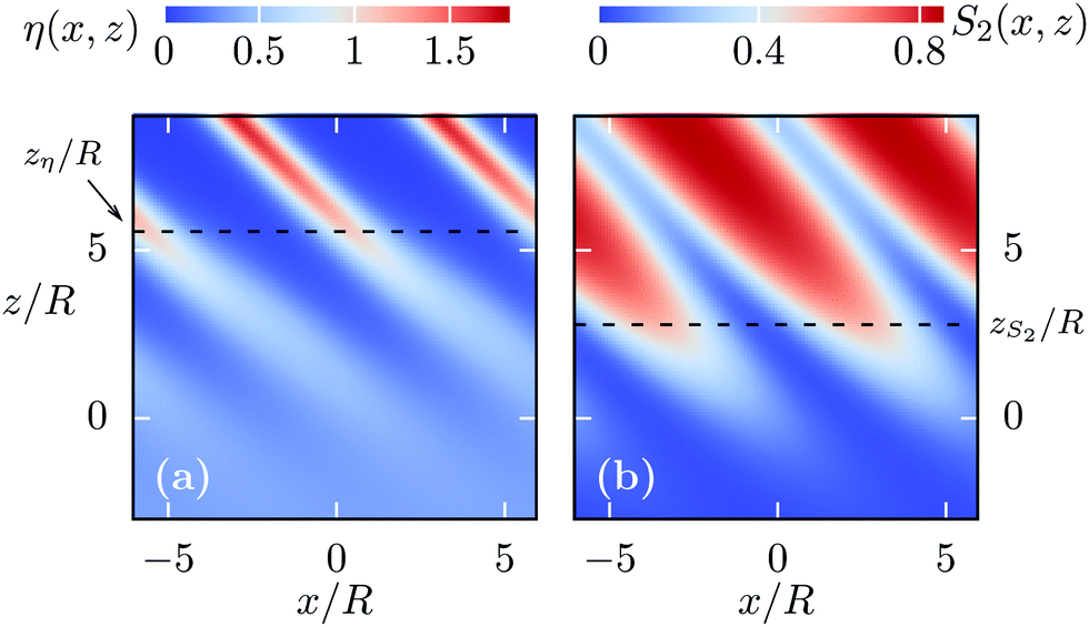 | ||
| Fig. 12 The L–SA interface profiles η(x,z) (eqn (20)) and S2(x,z) (eqn (21)) for α = π/4 and T* = 1.3 are shown. Here, an ILC with charges localized at its center is considered (L/R = 4, εR/εL = 2, γ/(Rε0) = 0.045, λD/R = 5, and D = 0). For z → −∞ the isotropic liquid bulk L is approached and for z → ∞ the bulk of the SA phase is attained, i.e., the interface normal is parallel to the z-axis. The red stripes at the top of the contour plots show the tails of the smectic layers. The black dashed lines mark the interface positions zη/R ≈ 5.56 and zS2/R ≈ 2.79 calculated viaeqn (23) and (24). Similar to the case α = π/2 (see Fig. 8), to a certain extent the orientational order persists into the liquid phase L. | ||
In Fig. 13 the interfacial tension Γ*(α) given by eqn (26) and the distance zη − zS2 between the interface positions associated with the mean packing fraction η0(x) and the mean orientational order parameter S20(x) are shown as function of the tilt angle α. In Fig. 13(a) the case of the L–SA-interface for ILCs with the charges at their center is considered for T* = 1. Both the interfacial tension Γ*(α) (black dots, •) and the distance zη − zS2 (orange dots,  ) exhibit a global minimum at α = 0 and a second, local minimum at α = π/2. Thus, the equilibrium tilt angle αeq = 0 corresponds to the configuration in which the interface normal and the smectic layer normal = ẑ are parallel, whereas the corresponding perpendicular orientation α = π/2 is metastable. This increase in the interfacial tension Γ* below α = π/2 suggests that the configuration, in which the interface normal and the layer normal are orthogonal, should be observable without resorting to any external stabilizing field which could be provided, e.g., by a suitably structured substrate. This metastability of the tilt angle α = π/2 can be checked also via computer simulations. Interestingly, the increase of the interfacial tension below α = π/2 is accompanied by an increase in the distance zη − zS2, suggesting that maintaining the local orientational order in the isotropic liquid beyond the smectic layers costs free energy. Consistently, in the case αeq = 0, for which the orientational order vanishes directly with the disappearance of the smectic layers, the cost in free energy is lowest. Apparently, for α = 0 the interfacial tension Γ*(α = 0) ≈ 0.006 is significantly smaller than for all other angles α shown in Fig. 13(a). For technical reasons we did not study small tilt angles α > 0 and hence cannot comment on the functional form of Γ*(α) for 0 < α < π/6 in the case D/R = 0 or for 0 < α < π/4 in the case D/R = 1.8. This is indicated by connecting the data points at α = 0 and π/6 by dashed lines. (For the same reason, in (b) the data points at α = 0 and π/4 are connected by dashed lines.) It has been pointed out in Section 2.2, that due to the crossover at the tilt angle α = 0 from a periodic system towards one which is translationally invariant in lateral direction x, the integration domain d for evaluating the coefficients Qi(r) (see eqn (16)) is not continuously evolving at α = 0. For α > 0 it is a slice of length dx = d/sin(α) in x-direction, while for α = 0 it is the subsystem of length d in z-direction at position r. (For α = 0 the extent in x- and y-direction is arbitrary due to the translational invariance in lateral direction.) In order to describe a continuous variation of the interfacial tension Γ*(α) for all tilt angles α ∈ [0,π/2], one thus needs to consider a different approach, which does not rely on a projected density and thereby on the direction of the bulk smectic layer normal throughout the whole interface structure. Nonetheless, our above approach still allows one to compare the interfacial tension Γ*(α) for the extreme cases α = 0 and π/2, thus predicting which one of the two is preferred. Furthermore, our approach provides an understanding of the local increase in Γ*(α) below α = π/2, as one observes an increasing distance zη − zS2 between the transition in the structural and the orientational order at the interface.
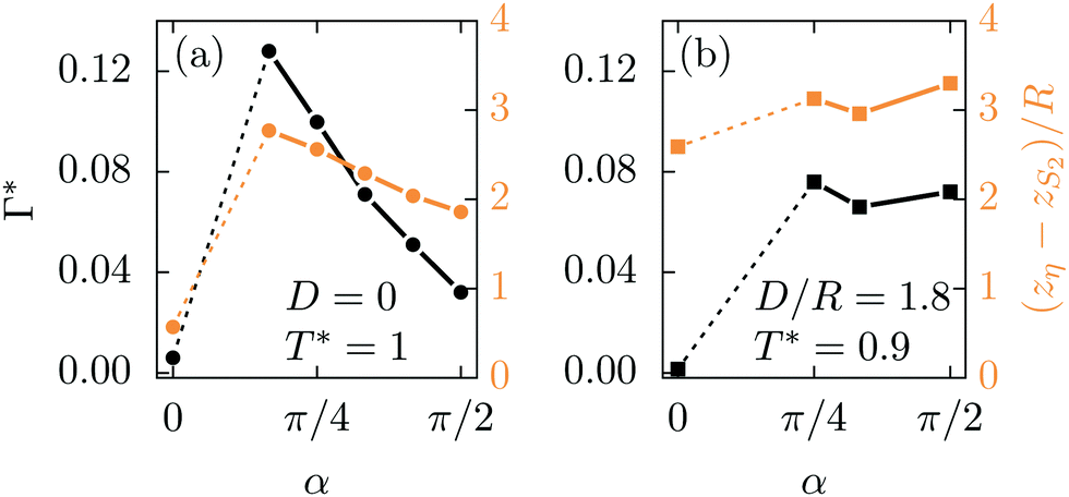 | ||
| Fig. 13 The (reduced) interfacial tension Γ*(α) (eqn (26), black line) and the distance zη − zS2 between the transition in the structural and the orientational order (orange line) as function of the tilt angle α. In panel (a) the L–SA interface at T* = 1 is considered for ILCs with their charges localized at the center (L/R = 4, εR/εL = 2, γ/(Rε0) = 0.045, λD/R = 5, and D = 0 (see Fig. 4(a)). There are two minima: the global minimum at the equilibrium tilt angle αeq = 0 (i.e., interface normal and smectic layer normal are parallel) and a local minimum at α = π/2 which shows that the orthogonal orientation of the smectic layer normal and the interface normal is a metastable configuration. The increase of the interfacial tension below α = π/2 is accompanied by an increase of the distance zη − zS2. This suggests that maintaining to a certain extent the local orientational order in the isotropic liquid beyond the smectic layers costs free energy. For technical reasons we did not study small tilt angles α > 0. Hence we cannot comment on the functional form of Γ*(α) for 0 < α < π/6 in the case D/R = 0 or for 0 < α < π/4 in the case D/R = 1.8. This is indicated by connecting the data points at α = 0 and π/6 by dashed lines in (a) (see the discussion in the main text of Section 3.4). In panel (b) the L–SAW interface, which is accessible for ILCs with their charges at the tips (L/R = 4, εR/εL = 2, γ/(Rε0) = 0.045, λD/R = 5, and D/R = 1.8), is considered for T* = 0.9 (see Fig. 4(b)). Also in this case the equilibrium tilt angle αeq = 0 corresponds to the parallel orientation of the interface normal and the layer normal. Below α = π/2, as function of α the interfacial tension is rather flat, taking the value Γ* ≈ 0.07. Thus, for the L–SAW interface the perpendicular orientation of the interface normal and of the smectic layer normal corresponds to a labile configuration. (Analogously to panel (a), the data points at α = 0 and π/4 in (b) are connected by a dashed line.) We note that Γ*(α) is symmetric around α = π/2, due to the mirror-symmetry of the particles. | ||
Fig. 13(b) shows data for the L–SAW-interface at T* = 0.9 for ILCs with charges located at the tips. Around α = π/2 the interfacial tension (black squares, ■) is a rather flat function of α taking values around Γ* ≈ 0.07. The slight variations in Γ* for α ∈ [π/4,π/2] might be caused by the numerical evaluation of eqn (8) which has to be done separately for each tilt angle α. Consistently, the distance zη − zS2 (orange squares,  ) does not vary much as function of the tilt angle α. As above, the equilibrium tilt angle αeq = 0 corresponds to the configuration in which the interface normal and the smectic layer normal = ẑ are parallel.
Finally, in Fig. 14, we show the contour plot of the L–SAW-interface for α = π/3 and T* = 0.9 for an ILC system with D/R = 1.8, illustrating the structure of this type of interface.
 | ||
| Fig. 14 Same as Fig. 12. Here, the L–SAW interface profiles η(x,z) (eqn (20)) and S2(x,z) (eqn (21)) are shown for α = π/3 and T* = 0.9. To this end, an ionic liquid crystal with charges at the tips is considered (L/R = 4, εR/εL = 2, γ/(Rε0) = 0.045, λD/R = 5, and D/R = 1.8). For z → −∞ the isotropic liquid bulk L is approached and for z → ∞ the bulk of the SAW phase, i.e., the interface normal is parallel to the z-axis. The transition in the structure occurs at zη/R ≈ 2.28 and the transition in the orientational order does so at zS2/R ≈ −0.68. | ||
4 Summary and conclusions
Free interfaces in systems composed of ionic liquid crystals (ILCs) have been studied within density functional theory (see Section 2.2). In particular, the discussion has been focused on two kinds of ionic liquid crystals: first, ILCs with the charges localized at the center of the molecules, i.e., D = 0 (see Fig. 1 and 2), and, second, ILCs with the charges at the tips of the molecules, i.e., D/R = 1.8. All other model parameters, i.e., L/R = 4, εR/εL = 2, γ/(Rε0) = 0.045, λD/R = 5, are identical in both cases. Therefore the two kinds differ solely by the charge distribution within the molecules.For D = 0 coexistence between the isotropic liquid L and the ordinary smectic-A phase SA can be observed at a sufficiently large mean packing fraction η0 (see Fig. 4(a)). The SA phase is characterized by a layered structure in the direction of the smectic layer normal with a smectic layer spacing d ≈ L comparable to the particle length L. Within the smectic layers the particles are well aligned with the smectic layer normal. The phase behavior of ILCs is altered by varying the molecular charge distribution, as can be inferred from comparing the case D = 0 (i.e., charges at the center) and D/R = 1.8 (i.e., charges at the tips, see Fig. 4(b)). At sufficiently low temperatures a new smectic-A phase has been observed, which is referred to as the SAW phase.11 The SAW phase shows an alternating structure of layers with the majority of the particles being oriented parallel to the smectic layer normal and the minority of the particles localized in secondary layers which prefer orientations perpendicular to . Due to the alternating layer structure, the smectic layer spacing d/R ≈ 7.5 in the SAW phase is increased compared with the spacing in the SA phase.
For a parallel orientation of the smectic layer normal = ẑ and the L–SA-interface normal, i.e., for α = 0 (see Fig. 3), it turns out that the interface locations zη and zS2, associated with the transition in the structural and in the orientational order, respectively, are very close to each other (see Fig. 5). In fact, Fig. 6 shows that for the whole temperature range considered here, the difference zη − zS2 < d in the two interface positions is smaller than the smectic layer spacing d. Hence, for α = 0 the orientational order vanishes within the last smectic layer at the L–SA-interface. Concerning the interface positions, Fig. 6 demonstrates that ILCs with D/R = 1.8 and ordinary (uncharged) liquid crystals with L/R = 4 and εR/εL = 2 exhibit qualitatively the same results. Considering the L–SAW-interface (see Fig. 7) one observes an increase in zη − zS2, but it remains significantly smaller than the smectic layer spacing d/R ≈ 7.5. Thus, for α = 0 it turns out that the loss of orientational order coincides with the disappearance of the layer structure of the respective smectic-A phase at the interface towards the isotropic liquid. This holds for all parameter values studied here.
Interestingly, for α = π/2, i.e., changing the relative orientation of the smectic layer normal = and the interface normal such that they are perpendicular to each other, leads to qualitative changes in the interfacial properties: a periodic structure of the interface in lateral direction x can be observed, which is a direct consequence of the periodicity in the bulk smectic-A phase with the smectic layer spacing d (see Fig. 3, 8, and 9). For the L–SA-interface (see Fig. 8) one observes considerable differences (zη − zS2)/R ≳ 2 between the interface positions. Thus, the (nearly) parallel orientations of particles in the SA layers persists a few particle diameters R into the liquid phase L, unlike the case α = 0, for which the orientational order vanishes directly with the breakdown of the SA layer structure at the interface, i.e., within the last smectic layer. Due to the periodicity in (lateral) x-direction, in the case α = π/2 one indeed observes a qualitative change in the structure of the L–SAW-interface compared to the L–SA-interface. While at the tails of the SAW main layers the interface also features an orientational order which continues further into the liquid phase L than the layer structure ((η(x) − S2(x))/R ≈ 2.6). For the secondary layers it is the layer structure that persists deeper into the L phase than the orientational order ((η(x) − S2(x))/R ≈ −3.73). The opposite behavior at the main, respectively secondary, layers is presumably driven by the orientational properties of the respective kinds of layers: in the main layers the particles are well aligned with the smectic layer normal = and therefore show an effective diameter in the y−z-plane which is comparable to the particle diameter R. However, in the secondary layers (here with S2(x,z) < 0) the particles avoid orientations parallel to the x-axis, giving rise to an considerably larger effective radius. Upon approaching the liquid phase L, this effective radius increases for the main layers of the SAW phase, whereas it decreases for the secondary layers.
In Section 3.3 the asymptotic behavior of the interface profiles has been studied. In particular, in Fig. 10 and 11 the L–SA-interface for α = π/2 has been considered for the two ILC systems with D/R = 0 and 1.8. For D = 0, i.e., with the charges being localized at the center, the periodic structure of the interface is apparent from the quantities ln|η(x,z) − ηL| and ln|S2(x,z) − S2,L|, showing the logarithmic deviations of the profiles η(x,z) and S2(x,z) from their respective liquid bulk values ηL and S2,L (Fig. 11(a) and (b)), which can be resolved even at far distances z/R < −20 from the L–SA-interface. Conversely, for D/R = 1.8, i.e., the charges being fixed at the tips, far from the interface ln|η(x,z) − ηL| and ln|S2(x,z) − S2,L| vary only marginally as function of the lateral coordinate x. While for D = 0 the charges are strongly localized at the centers of the smectic layers, thus promoting the periodic structure, for D/R = 1.8 the charges are less localized and more distributed along the x-direction.
The asymptotic decays of the interface profiles towards the isotropic liquid L show an interesting and rich behavior. We have found three distinct spatial regimes, which are associated with the three contributions to the underlying pair potential (see eqn (1)). Although the presence of charges is the distinctive feature of ILCs, the (screened) electrostatic contribution to the interaction (eqn (5)) governs the asymptotic decay only at intermediate distances from the interface (see Fig. 11). In this regime, the decay length is given by the Debye screening length, here λD/R = 5. Ultimately, it is the attractive Gay–Berne contribution to the interaction (eqn (2)) which dominates the outermost asymptotic behavior; for the system studied here a considerably large decay length ξGB/R ≈ 10 is observed, which is due to the truncated power law decay of the GB potential. Close to the interface, the hard-core interaction, which leads to the Parsons–Lee contribution to the DFT expression (eqn (12)), dominates the profiles η(x,z) and S2(x,z). The corresponding decay length ξPL/R ≈ 1.9 is comparable to the particle diameter R. This is plausible, because for the case considered here the tilt angle is α = π/2, i.e., the smectic layer normal is perpendicular to the interface normal, and thus the particles in the SA layers are oriented preferentially perpendicular to the interface normal as well. Interestingly, the crossovers between these three different regimes occur at distances characteristic for the packing fraction η(x,z) and the orientational order parameter S2(x,z). While for both types of ILCs considered in Fig. 11 all three decay lengths ξPL, ξGB, and λD are apparent from ln|S2(x,z) − S2,L|, from ln|η(x,z) − ηL| only the decay length λD can be inferred within the considered range z/R > −80. This situation is caused by the relative magnitudes of the respective decay amplitudes: for the packing fraction profile the decay amplitudes due to the Gay–Berne and the hard-core interaction are too small, compared to the corresponding amplitude due to the electrostatic interaction, to be observable.
Since the structural and orientational properties directly at the interface position are determined by the hard-core interaction, i.e., the Parsons–Lee contribution βψPL (eqn (12)), to the effective one-particle potential βψ, close to the interface the profiles for ordinary liquid crystals (OLCs) and ILCs with the same length-to-breadth ratio L/R are very similar. In particular, this includes the interface positions zη and zS2 (see Fig. 6) associated with the transition in the structural and orientational order, respectively. Nevertheless the asymptotic behavior, as discussed above, is distinct for the different kinds of particles (hard ellipsoids, OLCs, and ILCs) and shows a rich phenomenology, specifically for ILCs, due to the cross-overs between the distinct spatial regimes corresponding to the various contributions to the pair potential. Additionally, the bulk phase behavior is crucially affected by the type of particles, because only for the ILCs with charges at the tips, the phase SAW is observed.
Finally, the dependence of the structural and orientational properties of liquid–smectic interfaces on the tilt angle α between the interface normal and the smectic layer normal has been discussed. For the L–SA-interface (see Fig. 13(a)), it turns out, that the parallel orientation of the interface normal and of the smectic layer normal is the one in thermal equilibrium, i.e., αeq = 0. The perpendicular orientation α = π/2 is metastable. Interestingly, the increase in the interfacial tension below α = π/2 is accompanied by an increase in the distance zη − zS2, suggesting that maintaining the local orientational order beyond the smectic layers towards the isotropic liquid costs free energy. Consistently, in the case αeq = 0, for which the orientational order vanishes directly with the disappearance of the smectic layers, the cost of free energy for forming the interface is lowest. For the L–SAW-interface (see Fig. 13(b)) again the equilibrium tilt angle αeq = 0 corresponds to the parallel orientation of the interface and smectic layer normal. However, in this case, around α = π/2, the interfacial tension Γ*(α) varies only weakly so that here the perpendicular orientation is labile. Additional contributions to the surface tensions might arise from elastic deformations of the director field, i.e., spatial variations of the director := (r), or deviations from a rotational-symmetric distribution of particle orientations around the director, i.e., f(r,ω) ≠ f(r, ·ω). These contributions are neglected by our approach. Elastic effects can be considered through an explicit dependence of the free energy functional on the director field n(r), i.e., via an elastic energy contribution.50 Alternatively, giving up the assumption of a rotational symmetric distribution of orientations around a particular axis (and thereby enforcing a prescribed homogeneous director field) would also allow one to study the deformations of the director field. However, incorporating these effects would lead to a drastic increase of the computational effort.
Lastly, we emphasize that although here we have focused solely on free interfaces between coexisting bulk phases of ILCs, the DFT framework in Section 2.2 can be extended to inhomogeneous systems of ILCs exposed, e.g., to external fields or ILC–electrolytes in contact with an electrode.
Conflicts of interest
There are no conflicts to declare.Appendix A Implications of the presence of odd Fourier modes in ![[small rho, Greek, macron]](https://www.rsc.org/images/entities/h3_i_char_e0d1.gif) (r,ω)
(r,ω)
In this appendix the implications are discussed of considering the occurrence of odd Fourier modes up to second-order ones within the projected density (r,ω). Including these terms, (r,ω) takes the following modified form: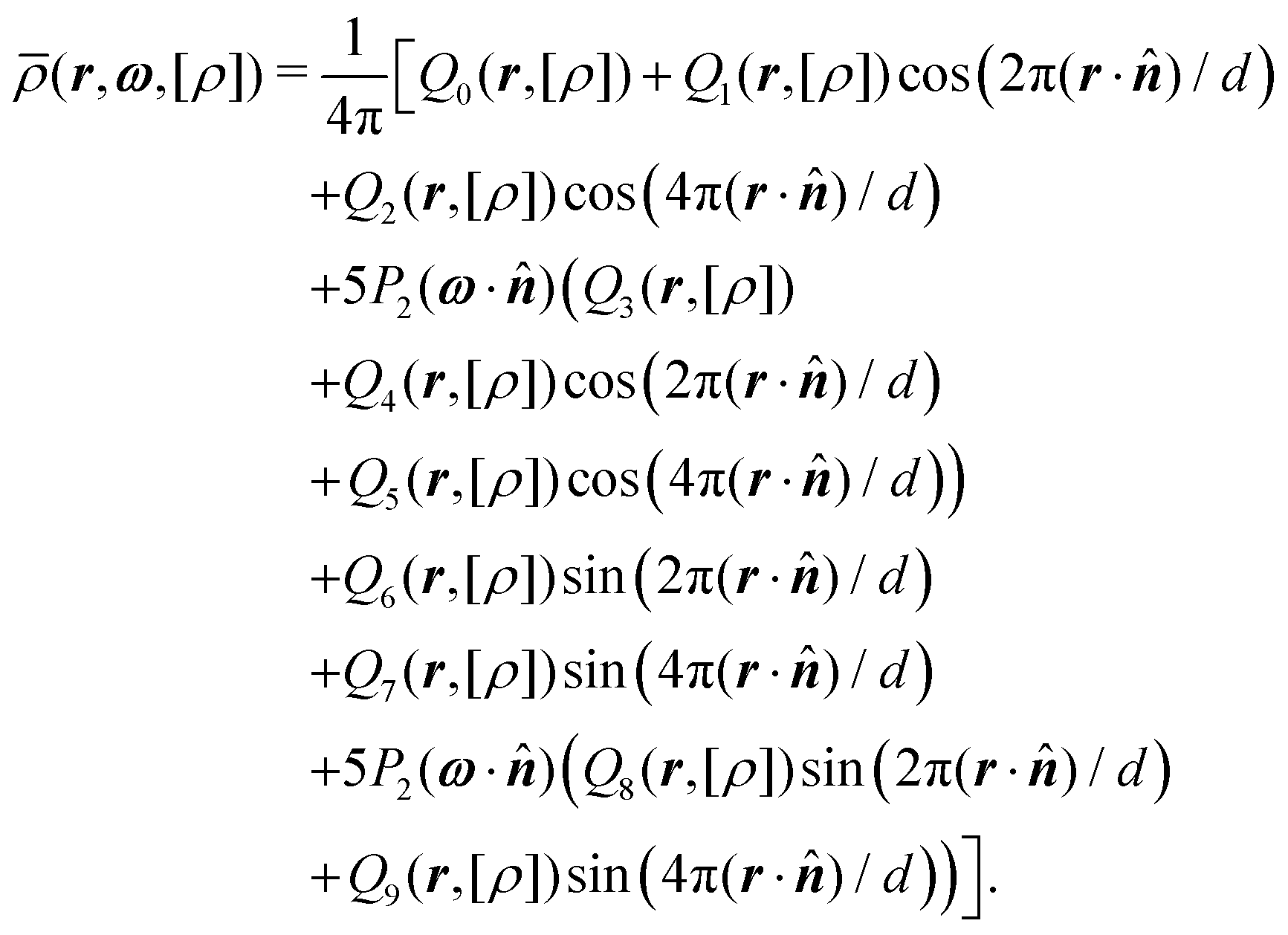 | (27) |
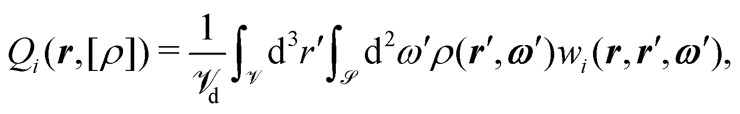 | (28) |
The coefficients Qi with i = 6,…,9 vanish for the considered bulk phases, because smectic-A phases exhibit mirror-symmetry with respect to the layer center. In general, at interfaces they do not vanish. In order to compare the corresponding interface profiles

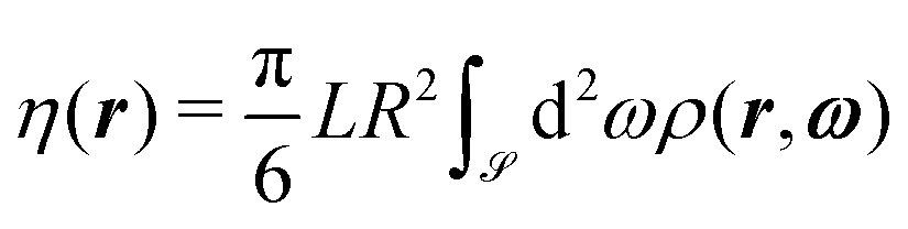 and
and  (see eqn (20) and (21), respectively; is the full solid angle) obtained from solving the Euler–Lagrange equation, i.e., eqn (8), by using the projected density without the odd terms given by eqn (11) and the projected density containing these terms, i.e., by using eqn (28), the case α = π/3 (see eqn (15)) and the L–SAW-interface shown in Fig. 14 are considered again. In Fig. 15 the two respective profiles are shown by using eqn (27): for both η(r) and S2(r) there are no qualitative differences compared with Fig. 14. The interface positions zη/R ≈ 0.24 and zS2/R ≈ −2.23 are shifted in z-direction compared to the results shown in Fig. 14. But their distance (zη − zS2)/R ≈ 2.47 is comparable to the previous results ((zη − zS2)/R ≈ 2.96 in Fig. 14). Hence, in qualitative agreement with the results shown in Fig. 14 one observes a persisting orientational order (within the main layers of the SAW phase) up to a few particle diameters R into the liquid phase.
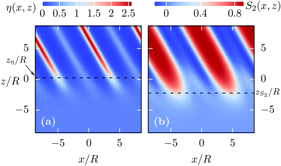 | ||
| Fig. 15 Same as Fig. 14. Here, the L–SAW interface profiles η(x,z) (eqn (20)) and S2(x,z) (eqn (21)) are calculated for α = π/3 and T* = 0.9 by using the projected density containing odd Fourier-modes up to second order. The profiles are qualitatively equivalent to those obtained without using the odd modes in the projected density (r,ω) (see eqn (11)). In agreement with the results shown in Fig. 14 one observes an orientational order (within the main layers of the SAW phase) persisting up to a few particle diameter R into the liquid phase ((zη − zS2)/R = 0.24 − (−2.23) = 2.47). | ||
Acknowledgements
Open Access funding provided by the Max Planck Society.Notes and references
- K. Binnemans, Chem. Rev., 2005, 105, 4148–4204 CrossRef CAS PubMed.
- C. J. Bowlas, D. W. Bruce and K. R. Seddon, Chem. Commun., 1996, 1625–1626 RSC.
- K. Goossens, K. Lava, C. W. Bielawski and K. Binnemans, Chem. Rev., 2016, 116, 4643–4807 CrossRef CAS PubMed.
- C. M. Gordon, J. D. Holbrey, A. R. Kennedy and K. R. Seddon, J. Mater. Chem., 1998, 8, 2627–2636 RSC.
- K.-M. Lee, Y.-T. Lee and I. J. B. Lin, J. Mater. Chem., 2003, 13, 1079–1084 RSC.
- D. Ster, U. Baumeister, J. L. Chao, C. Tschierske and G. Israel, J. Mater. Chem., 2007, 17, 3393–3400 RSC.
- N. Yamanaka, R. Kawano, W. Kubo, T. Kitamura, Y. Wada, M. Watanabe and S. Yanagida, Chem. Commun., 2005, 740–742 RSC.
- M. Wang, X. Pan, S. Xiao, C. Zhang, W. Li and S. Dai, J. Mater. Chem., 2012, 22, 2299–2305 RSC.
- N. Yamanaka, R. Kawano, W. Kubo, N. Masaki, T. Kitamura, Y. Wada, M. Watanabe and S. Yanagida, J. Phys. Chem. B, 2007, 111, 4763–4769 CrossRef CAS PubMed.
- S. Kondrat, M. Bier and L. Harnau, J. Chem. Phys., 2010, 132, 184901 CrossRef.
- H. Bartsch, M. Bier and S. Dietrich, J. Phys.: Condens. Matter, 2017, 29, 464002 CrossRef PubMed.
- L. Mederos and D. E. Sullivan, Phys. Rev. A: At., Mol., Opt. Phys., 1992, 46, 7700–7707 CrossRef.
- A. M. Somoza, L. Mederos and D. E. Sullivan, Phys. Rev. E: Stat. Phys., Plasmas, Fluids, Relat. Interdiscip. Top., 1995, 52, 5017–5027 CrossRef CAS.
- Y. Martinez-Raton, E. Velasco, A. M. Somoza, L. Mederos and T. J. Sluckin, J. Chem. Phys., 1998, 108, 2583–2593 CrossRef CAS.
- D. de las Heras, E. Velasco and L. Mederos, Phys. Rev. Lett., 2005, 94, 017801 CrossRef CAS PubMed.
- S. Wolfsheimer, C. Tanase, K. Shundyak, R. van Roij and T. Schilling, Phys. Rev. E: Stat., Nonlinear, Soft Matter Phys., 2006, 73, 061703 CrossRef CAS PubMed.
- H. Reich, M. Dijkstra, R. van Roij and M. Schmidt, J. Phys. Chem. B, 2007, 111, 7825–7835 CrossRef CAS PubMed.
- S. Praetorius, A. Voigt, R. Wittkowski and H. Löwen, Phys. Rev. E: Stat., Nonlinear, Soft Matter Phys., 2013, 87, 052406 CrossRef PubMed.
- M. E. Fisher and Y. Levin, Phys. Rev. Lett., 1993, 71, 3826–3829 CrossRef CAS PubMed.
- M. E. Fisher, J. Stat. Phys., 1994, 75, 1–36 CrossRef.
- E. Luijten, M. E. Fisher and A. Z. Panagiotopoulos, Phys. Rev. Lett., 2002, 88, 185701 CrossRef PubMed.
- V. Kobelev, A. B. Kolomeisky and M. E. Fisher, J. Chem. Phys., 2002, 116, 7589–7598 CrossRef CAS.
- F. H. Stillinger and R. Lovett, J. Chem. Phys., 1968, 48, 3858 CrossRef CAS.
- F. H. Stillinger and R. Lovett, J. Chem. Phys., 1968, 49, 1991 CrossRef CAS.
- R. Lovett and F. H. Stillinger, J. Chem. Phys., 1968, 48, 3869–3884 CrossRef CAS.
- D. Mitchell, D. A. McQuarrie, A. Szabo and J. Groeneveld, J. Stat. Phys., 1977, 17, 15–20 CrossRef.
- L. Harnau and P. Reineker, J. Chem. Phys., 2000, 112, 437–441 CrossRef CAS.
- G. Stell, K. C. Wu and B. Larsen, Phys. Rev. Lett., 1976, 37, 1369–1372 CrossRef.
- M. J. Gillan, Mol. Phys., 1983, 49, 421–442 CrossRef CAS.
- R. Dickman and G. Stell, AIP Conf. Proc., 1999, 492, 225–249 CAS.
- G. Wulff, Kristallogr. Mineral., 1901, 34, 449 CAS.
- C. Blanc, Phys. Rev. E: Stat., Nonlinear, Soft Matter Phys., 2001, 64, 011702 CrossRef CAS PubMed.
- B. J. Berne and P. Pechukas, J. Chem. Phys., 1972, 56, 4213–4216 CrossRef CAS.
- J. G. Gay and B. J. Berne, J. Chem. Phys., 1981, 74, 3316–3319 CrossRef CAS.
- G. Saielli, T. Margola and K. Satoh, Soft Matter, 2017, 13, 5204–5213 RSC.
- R. Berardi, A. P. J. Emerson and C. Zannoni, J. Chem. Soc., Faraday Trans., 1993, 89, 4069–4078 RSC.
- M. A. Bates and G. R. Luckhurst, J. Chem. Phys., 1999, 110, 7087–7108 CrossRef CAS.
- P. Tarazona, Phys. Rev. A: At., Mol., Opt. Phys., 1985, 31, 2672–2679 CrossRef CAS.
- J. D. Parsons, Phys. Rev. A: At., Mol., Opt. Phys., 1979, 19, 1225–1230 CrossRef.
- S. Lee, J. Chem. Phys., 1987, 87, 4972–4974 CrossRef CAS.
- J. P. Hansen and I. R. McDonald, Theory of Simple Liquids, Academic, San Diego, 1986 Search PubMed.
- L. Onsager, Ann. N. Y. Acad. Sci., 1949, 51, 627–659 CrossRef CAS.
- R. van Roij, Eur. J. Phys., 2005, 26, S57 CrossRef CAS.
- P. I. Teixeira and M. M. Telo da Gama, J. Phys.: Condens. Matter, 1991, 3, 111 CrossRef CAS.
- R. Evans, Adv. Phys., 1979, 28, 143–200 CrossRef CAS.
- B. Q. Lu, R. Evans and M. M. Telo da Gama, Mol. Phys., 1985, 55, 1319–1338 CrossRef CAS.
- P.-G. de Gennes, J. Phys., Lett., 1981, 42, 377–379 CrossRef CAS.
- J. A. Barker and J. R. Henderson, J. Chem. Phys., 1982, 76, 6303–6307 CrossRef CAS.
- S. Dietrich and M. Napiórkowski, Phys. Rev. A: At., Mol., Opt. Phys., 1991, 43, 1861–1885 CrossRef CAS.
- P.-G. de Gennes and J. Prost, The Physics of Liquid Crystals, Clarendon, Oxford, 1974 Search PubMed.
| This journal is © The Royal Society of Chemistry 2019 |