Surface relief of magnetoactive elastomeric films in a homogeneous magnetic field: molecular dynamics simulations

Abstract

The structure of a thin magnetoactive elastomeric (MAE) film adsorbed on a solid substrate is studied by molecular dynamics simulations. Within the adopted coarse-grained approach, a MAE film consists of magnetic particles modeled as soft-core spheres, carrying point dipoles, connected by elastic springs representing a polymer matrix. MAE films containing 20, 25 and 30 vol% of randomly distributed magnetic particles are simulated. Once a magnetic field is applied, the competition between dipolar, elastic and Zeeman forces leads to the restructuring of the layer. The distribution of the magnetic particles as well as elastic strains within the MAE films are calculated for various magnetic fields applied perpendicular to the film surface. It is shown that the surface roughness increases strongly with growing magnetic field. For a given magnetic field, the roughness is larger for the softer polymeric matrix and exhibits a nonmonotonic dependence on the magnetic particle concentration. The obtained results provide a better understanding of the MAE surface structuring as well as possible guidelines for fabrication of MAE films with a tunable surface topology.

---

1 Introduction

Magnetoactive elastomers (MAEs) are composite smart materials consisting of soft polymeric matrices with embedded magnetic microparticles. They are the subject of growing interest nowadays because of the rich variety of physical phenomena observed under the action of external magnetic fields and their numerous promising technological applications (see reviews ref. 1–6).

The basis of MAE “smartness” lies in the coupling of magnetic and elastic components of these materials. This coupling becomes important when the polymeric matrix is soft enough for the magnetic forces, acting between magnetic particles in a magnetic field, and elastic forces of the polymer matrix to be of the same order of magnitude. The softness of the polymer matrix, on the one hand, gives particles some freedom to move, so that they can shift from their zero field equilibrium positions in the course of interactions in a magnetic field; however, the particle mobility is still limited. The elastic constraints make the main difference in the behavior of magnetic elastomers and magnetic fluids that are based on liquid dispersing media. Liquid background ensures free movement of magnetic particles.^7,8 As a result, in the case of MAEs, the external magnetic field drives a restructuring of the magnetic filler within the polymer matrix while the final microstructure is defined by a balance between magnetic and elastic interactions.

Rearrangement of magnetic particles in MAEs with the formation of mesoscopic chain-like structures in magnetic fields has been reported in several publications. Owing to a micrometer size of the particles, it can be directly observed by means of optical microscopy.^9–13 Furthermore, an X-ray tomography has recently been applied to monitor particle displacements under the action of magnetic fields.^14–16 This technique allows one to reconstruct a three-dimensional map of the magnetic structures, to color every individual particle and to track its spatial position evolution induced by external stimuli.

It is a magnetic filler rearrangement in a magnetic field that is responsible for the high magnetic response of MAEs, that manifests as giant variations in magneto-mechanical as well as in magneto-electric properties of these composites. Magneto-mechanical response of MAEs is manifold. First of all, one should mention a giant magnetorheological effect, i.e., up to three-four orders of magnitude increase of the MAE elastic modulus under moderate magnetic fields of 0.5–0.6 T.^17–22 Then, considerable magnetodeformations are typical for MAEs both in uniform and gradient magnetic fields.^23–26 Furthermore, a kind of a shape memory effect, which is expressed as large residual deformations fixed by applied magnetic fields, was observed in ref. 11 and 12. This complex of magneto-mechanical features defines prospective MAEs applications as tunable dampers, vibration absorbers, seals, microactuators and even artificial muscles.⁴ Investigations of maneto-electric properties of MAEs have been started more recently.^27–30 It has been shown that the effective dielectric constant as well as conductivity of MAEs can be tuned by external magnetic fields.³⁰ This fact opens up new ways of MAEs practical applications, in particular, as magnetic field sensors.

It has been mentioned in ref. 28 that any bulk property of MAEs which is dependent on the internal structure of filler particles could be influenced by magnetic fields. On the other hand, it has been shown recently that magnetic fields can also alter the surface properties of magneto-polymer composites. In particular, application of a magnetic field perpendicular to the surface of films made of MAEs induces formation of needle-like or mountain-like structures on their surface.^31,32 Note that the presence of a hard magnetically passive substrate makes the deformation anisotropic and magnifies the surface effects. The scanning electron microscopy study of MAE films based on PDMS containing 10–30 vol% of carbonyl iron particles cured in various magnetic fields has shown that the resulting surface morphology depends on the strength of the magnetic field applied in the course of curing.³¹ Furthermore, the surface relief of initially isotropic MAE films can finely be tuned by an external magnetic field even after curing³² if the polymer matrix is soft enough to allow filler alignment with the field. Chains of magnetic particles could grow and extend from the inner region of the material to its surface, producing some mountain-like surface structure. The increased roughness of MAE surface causes a change in wettability and adhesion properties of MAE films. It has been demonstrated in ref. 32 that the water contact angle on a MAE surface can increase from 110° at zero magnetic field up to 163° in magnetic fields of 600 mT. This effect can be called as “magneto-hydrophobicity” or “magneto-superhydrophobicity” of MAEs. In the aforementioned works, the coatings with a thickness on the order of 100–200 μm were studied. Magnetic particles had an average size of 5 μm and were magnetically soft. In other words, the layer thickness was approximately 20–40 particles diameters. Tunable surface roughness and wettability of soft MAEs have also been reported in ref. 33, however, despite the increased surface roughness, the apparent contact angle has shown to decrease with increasing field. This fact has been attributed to the field-induced protrusion of hydrophilic iron particles from the surface layer. Anyway, the first reported results^31–33 indicate that with MAEs it is possible not only to produce hydrophobic coatings by applying an external magnetic field in the course of curing, but also to dynamically tune the MAE wettability and control their magneto-hydrophobicity with magnetic fields. Stimuli-responsive surfaces like these attract much attention nowadays^34–36 due to their potential for the creation of new materials with advanced properties like self-cleaning, anti-sticking, anti-fouling, anti-icing, anti-fogging, drag reduction, etc.

For controlling the surface wettability of MAEs coatings it is necessary to elucidate the interrelation between the applied external fields and the response of the material. It is well established that the internal restructuring of the magnetic filler and, thus, the responsive properties of MAEs depend considerably on the type and concentration of magnetic particles as well as on the elasticity of polymer matrix. One can expect that the surface restructuring would also be influenced by these factors. Indeed, in ref. 32 it has been shown that the surface hydrophobicity increases with iron filler content and with softening of the polymer matrix. To control the surface relief and thus, the wettability of MAE coatings it is essential to predict how the surface restructuring depends on the MAE characteristics as well as on the strength of the external magnetic field.

Hand in hand with the growing interest on the creation of magnetic materials and the development of advanced experimental characterisation techniques,^37–39 theoretical studies on magnetic elastomers are experiencing a considerable growth in recent years. Closely related to the modelling of magnetic gels, theoretical approaches to the study of magnetic elastomers include mean-field and continuum analytical theories,^26,40–43 as well as several approaches based on coarse-grained modelling by means of computer simulations. Besides few exceptions,⁴⁴ simulation models usually represent the embedded magnetic particles as beads with point magnetic dipoles, whereas the polymer matrix is modelled with different levels of detail. The most simple models use an implicit representation of the matrix, assuming affine deformations.^45,46 However, most simulation approaches use elastic springs to represent the mechanical constraints imposed by the polymer matrix on the magnetic particles, either using some fixed reference frame^16,39 or simply forming an interconnected network of particles and springs.^44,47–52 More detailed approaches use an explicit bead-spring representation of the polymers forming the matrix, at the cost of a much higher computational load.^53–56

In this paper we address the surface topology of a MAE coating via computer simulations. Using a coarse-grained approach based on a simple particle-spring network representation, we model a 3D thin layer of a magnetic polymer composite material attached to a flat substrate and study how the relief of its free surface depends on the strength of an applied magnetic field perpendicular to the substrate. We keep the ratio between the layer thickness and particle size close to that in ref. 32, but, for simplicity, we use magnetically hard particles in the simulations. Even though we are not aiming at the quantitative comparison with the experimental data, the high-field regime in our model reflects the qualitative behaviour of MAEs with magnetically soft particles, whereas the low field regime reveals the structural transformations that take place in magnetic elastomers with magnetically hard particles whose synthesis is currently in progress. We demonstrate that the proposed coarse-grained approach is able to catch the main features of the field-induced restructuring of the magnetic filler, in particular, the formation of mountain-like profiles of the MAE surface. The model we developed allows one to look at the microscopic origin of the experimentally observed changes in the surface properties of MAE coatings and to analyse the effects of the concentration of magnetic particles and the elasticity of the polymer matrix.

The paper is organised as follows. In the next section we describe the model and the method of simulation. Then we present the results, discussing the properties of the material and its surface depending on the applied magnetic field, magnetic particle concentration and matrix rigidity. Finally, we summarise the main conclusions and outlook.

2 Simulation model and method

In general, it is not feasible to model MAE materials at the atomistic or molecular scale, being the use of some coarse-grained approach unavoidable for computer simulations. Among the different levels of coarse-graining we discussed above, in this study we choose to represent the polymer matrix as a random network of elastic springs constraining the movements of the magnetic particles and to use molecular dynamics as the computer simulation technique.

In the following sections we introduce the details of our coarse-grained model of a MAE coating and the simulation method we employed.

2.1 Model interactions

The choice of a molecular dynamics simulation technique imposes the use of continuous interaction potentials in order to avoid unphysical artifacts when integrating the equations of motion. For this reason, we model magnetic particles in the elastomer as soft-core spheres of characteristic diameter σ. Specifically, the soft-core interaction is the Weeks–Chandler–Andersen (WCA) pair potential⁵⁷where U_LJ(r) is the conventional Lennard-Jones (LJ) potential with the potential well depth ε_sc, U_LJ(r;ε_sc,σ) = 4ε_sc[(σ/r)¹² − (σ/r)⁶], that in expression (1) is truncated at the position of its minimum, r_cut = 2^1/6σ, and shifted by its corresponding depth, U_LJ(r_cut), to make the interaction purely repulsive. The magnetic nature of these particles is represented by a permanent point dipole, [small mu, Greek, vector], located at their centers, whose orientation is fixed with respect to the particle body. The presence of the permanent dipoles makes the particles to interact by means of the conventional dipole–dipole pair potential,where r = |r⃑_ij| = |r⃑_i − r⃑_j| is the displacement vector between the centers of the interacting particles. This is a conventional approximation for spherical ferromagnetic particles, in general, and particularly accurate for the case of monodomain ones. However, the approximation can be also reasonably good for the case of superparamagnetic particles in the limit of strong homogeneous external fields. The application of any homogeneous external field, H⃑, affects the dipolar particles according to the Zeeman potential,

U_H([small mu, Greek, vector]_i,H⃑) = −[small mu, Greek, vector]_i·H⃑. (3)

This interaction will tend to induce rotations of the magnetic particles in order to align their dipoles with the field. For simplicity, here we do not constrain such rotations and consider only the translational constraints imposed by the polymer matrix. The latter is represented implicitly as a network of elastic constraints crosslinking the centres of the magnetic particles. In particular, we use a harmonic spring potential to crosslink them:where K is the elastic constant of the spring and R₀ is the equilibrium distance between the centers of the crosslinked particles.

2.2 Simulation approach

In order to mimic the magnetomechanical response of our model MAE coating, we use molecular dynamics simulations with a Langevin thermostat. Since we are dealing with a dry, rubber-like material, we perform our Langevin dynamics simulations at very low temperature, T, in order to obtain a nearly athermal relaxation of the system. The magnetic particles obey the translational and rotational Langevin equations, obtained by adding stochastic and friction terms to the Newtonian equations of motion:^58,59

m_i(d[small nu, Greek, vector]_i/dt) = F⃑_i − Γ_T[small nu, Greek, vector]_i + [small xi, Greek, vector]_i,T, (5)

I⃑_i·(d[small omega, Greek, vector]_i/dt) = [small tau, Greek, vector]_i − Γ_R[small omega, Greek, vector]_i + [small xi, Greek, vector]_i,R, (6)

where F⃑_i and [small tau, Greek, vector]_i are the total force and torque acting on the particle i, m_i is the particle mass and I⃑_i is its inertia tensor. Finally, Γ_T and Γ_R are the translational and rotational friction constants, and [small xi, Greek, vector]_i,T and [small xi, Greek, vector]_i,R are a Gaussian random force and torque, respectively, fulfilling the normal fluctuation–dissipation rules. Note that in this study we are not interested in reproducing the dynamics of the system, but only its static properties after magnetomechanical relaxation. Therefore, the values assigned to the friction constants are irrelevant for our discussion, leaving us the freedom to take the ones that provide a faster relaxation.

We use a cubic simulation box with side length L and lateral periodic boundaries in x and y directions, parallel to the film substrate. Magnetic interactions are calculated by means of the dipolar-P³M algorithm,⁶⁰ combined with the Dipolar Layer Correction method⁶¹ in order to take into account the slab geometry of the system.

We study elastomers with three different volume fractions of identical magnetic particles, ρ = {0.20,0.25,0.30}. This corresponds to 65–76 mass per cent in case of NdFeB in silicone. As it is usual in coarse-grained simulations, here we use a system of reduced units defined from the physical characteristics of the particles. Therefore, magnetic particles in our system have a reduced mass m_i = 1 and reduced diameter σ = 1. In this way, all lengths are measured in units of particle diameter. The reduced length of the simulation box side is fixed in all cases to L = 43.76. This value is chosen so that the thickness of a layer with homogeneously distributed particles and the highest sampled density, ρ = 0.30, does not exceed L/4. The amount of magnetic particles in each sample, N_p, calculated according to the aforementioned conditions for each increasing density, is N_p = {8000,10 000,12 000}, respectively.

Regarding energy scales, only the interplay between the magnetic interactions and the elastic constraints are relevant in our system. Therefore, we are free to choose any soft core energy scale that effectively hinders non reasonable particle overlaps. For simplicity, we take ε_sc = 1 as the reduced energy scale of the soft core interactions between magnetic particles, given by eqn (1). In the case of thermal fluctuations, defined by the product of the Boltzmann constant and the reduced temperature, kT, even though we are interested in an athermal regime, it is useful to keep a non zero temperature in the simulations in order to ease the relaxation of the system, preventing to let it get kinetically trapped into very stressed configurations. Besides this practical reason, the value of kT is also irrelevant as long as it is much lower than the rest of energy scales. Here we take kT = 10⁻³ for the main part of the simulations. For the magnetic interactions, we take a reduced dipole moment μ = 2 and sample external fields of reduced strengths up to H ≤ 7. Finally, the range of reduced constants for the elastic constraints, K, is between 0.001 and 0.1. The energy scales that stem from these choices for μ, H and K will be discussed in detail in the next section, together with the role of their interplay on the behaviour of the system.

Fig. 1 shows a sketch of a typical initial configuration of our elastomer coating model. The substrate is represented as a flat monolayer of non magnetic particles arranged into a fixed square lattice in the x−y plane, located at z = 0. These substrate particles interact with all magnetic particles only sterically, according to eqn (1), preventing the latter to cross the lower side of the simulation box. Since high field configurations of magnetic particles can exert very strong forces on the substrate, we take for this soft-core interaction a very high value of its prefactor, ε_sc = 10⁶. In close contact with the substrate, there is a layer of magnetic particles that can freely diffuse in the x−y plane, but their z-coordinate is fixed at z = 1. These particles represent the interface of the elastomer physically adsorbed on the substrate. The amount of particles belonging to this adsorbed layer is chosen to match the overall desired density, ρ. The rest of magnetic particles are found above the adsorbed layer, and can move in any direction. Elastic springs connect magnetic particles only. The way this initial configuration is prepared is the following. First, the chosen amount of magnetic particles, N_p, is placed randomly in the region between the substrate layer and a similar repulsive layer that is placed temporarily at z = L/4. The repulsive interaction of such top layer is also defined by eqn (1) with ε_sc = 10⁶. This system is then equilibrated in two simulation parts that exclude the calculation of magnetic interactions, using a fixed integration time step of δt = 0.001. In the first equilibration part, low temperature damped dynamics (T = 10⁻³, Γ = Γ_T = Γ_R = 100) are simulated until any strong overlap of the particles is removed. In the second part, further equilibration with moderate temperature and damping (T = 0.5, Γ = 10) is made for 2 × 10⁵ integration steps. This provides a homogeneous distribution of particles with the target density next to the substrate. At this point, the temporary repulsive top layer is removed and the particles are crosslinked. This is done by randomly selecting pairs of particles whose centre-to-centre distance is not larger than r ≤ 5 and adding a harmonic spring, with potential (4), connecting their centers. For each added spring the value of K is taken from a Normal distribution with mean K̄ and standard deviation s², N(K̄, s²), that is defined to span over a fixed arbitrary interval [K_min, K_max]. This is done by taking K̄ = (K_min + K_max)/2, s = (K_max − K_min)/6 and rejecting all values that do not lie within the chosen interval during the random picking. We sampled two different ranges for the rigidity constants: K = K_soft ∈ [0.001,0.01] and K = K_stiff ∈ [0.01,0.1]. In order to keep the volume fraction of the particles close to its chosen initial value when no external perturbation is applied, the equilibrium distance R₀, for each crosslinked pair is set to the value of r at the moment of establishing the crosslink. Any particle is allowed to have a maximum of 6 crosslinks. The crosslinks are added in this way up to the point when there are no more particle pairs left in the system that match the described criteria. By following this procedure, we observed that the vast majority of particles reach the maximum amount of crosslinks. In case some particle remains unconnected after the random picking, three springs are added connecting it to three close neigbouring particles. After this crosslinking procedure, another relaxation cycle of 2 × 10⁵ integration steps (T = 10⁻³, Γ = 10) is carried out.

Fig. 1 Sketch of the elastomer model. Magnetic particles are depicted with an arrow representing their dipole moment and elastic constraints as springs. The lowest layer of non magnetic particles is the substrate. The darker magnetic particles laying on the substrate are the adsorbed layer, i.e., they can only move in the plane of the substrate. All other magnetic particles can move in all three directions.

The final relaxation of the samples, including magnetic interactions, is performed according to the following protocol. Initially, dipoles of the particles are oriented randomly. In the first simulation cycle their moments are increased from μ = 0.1 to its final value μ = 2, in 10 cycles of 2 × 10³ integration steps each. Whenever an external field is applied, a similar stepwise increase of its value is performed at this point. Finally, the system is left to relax for 2.5 × 10⁵ integration steps. This amount of steps turned out to be sufficient for all systems to reach a state that we consider stationary, i.e., in which the total energy remains constant and any particle displacement becomes vanishingly small. Only the final configuration obtained from this protocol is used for the analysis. In order to obtain minimal statistics, all results presented here are averaged over 5 independent runs. The simulations were carried out with the package ESPResSo 3.3.1.^62,63

3 Results and discussion

We start the discussion of the results with the visual inspection of the simulation snapshots presented in Fig. 2. When no external magnetic field is applied, as is the case in Fig. 2(a), magnetic particles self-assemble into chain-like structures that seem to be predominantly oriented parallel to the substrate. This observation will be supported by formal calculations discussed below. The reason for the appearance of this structure is that dipolar interactions favour the formation of relatively long, preferably not too curved chains, as they maximise the amount of head-to-tail optimal dipole–dipole configurations. The formation of chains involves particles displacement from the positions that correspond to the equilibrium structure when no magnetic interactions are present. However, such displacements are opposed by the elastic constraints. Due to the finite size in z direction of the particle filled region and the high connectivity of the spring network, the formation of vertical chains longer than the thickness of the film can be only done statistically by large displacements of the topmost particles in the chain, i.e., by strongly stretching their springs. Indeed, such vertical stretching statistically grows with the chain length. The formation of long horizontal chains across the film instead can be achieved involving smaller displacements of the particles. Therefore, as an outcome of the competition between elastic and dipolar forces and the elastomer geometry, long chains oriented in-plane appear to be more energetically advantageous. The situation changes once a magnetic field perpendicular to the substrate is applied and the Zeeman contribution enters the competition, as shown in Fig. 2(b) to (d). The alignment of the dipoles with the field energetically compensates to certain extent the stretching of the springs required to form vertical chains of head-to-tail dipoles, thus such structure dominates under strong fields. This effect is more pronounced for the softer spring network. Vertical chains can form bundles in which neighbouring chains are not exactly parallel side-by-side, which makes unfavourable dipolar interactions, but vertically shifted by half particle diameter, as can be observed in the side views of the samples. Finally, one can also observe that the characteristic horizontal separation between chain bundles depends on both, the rigidity of the springs and the particle density: the softer are the springs and the less dense is the system, the larger is such separation, up to the point when the interstitial voids extend down to the substrate, as can be clearly seen in Fig. 2(d). These high field structures have a clear qualitative resemblance with scanning electron microscopy images of related experimental samples (see for instance Fig. 4 in ref. 32). Note that all the deformations in the present model are purely elastic and no irreversible breakage of the springs connecting the particles is allowed.

Fig. 2 Simulation snapshots obtained for selected sets of system parameters. In each panel, the top figure corresponds to the side view of the film and the lower figure to the top view. (a) ρ = 0.3, K_soft, H = 0. (b) ρ = 0.3, K_soft, H = 6. (c) ρ = 0.3, K_stiff, H = 6. (d) ρ = 0.2, K_soft, H = 6.

In the next sections we present a more detailed discussion on the system behaviour by means of the analysis of different parameters: energies, density profiles and film thickness, surface profile and roughness, and vertical distributions of elastic stresses. Finally, we will end the discussion by establishing the connection between our simulation results and the corresponding experimental systems.

3.1 System energies

The qualitative discussion on the competition between the three main energy contributions introduced above can be further formalised by computing their average values from simulation measurements. The top row of Fig. 3 presents the results for the run averages of the elastic (a), dipolar (b) and Zeeman (c) energies per particle as a function of the external magnetic field, H, for all sampled densities and matrix rigidities. Since we work with reduced units, only qualitative trends and quantitative differences or ratios for distinct system parameters, rather than specific individual values, are important for the discussion. The first observation one can extract from Fig. 3(a) to (c) is that all energies present two clear regimes: at low fields, there is a moderate change of the energies with field growth, whereas at high fields this change is significantly stronger. In some case (lowest density and rigidity) one can see an indication of elastic and dipole–dipole energies approaching saturation for the highest applied field, but in no case saturation regime is actually reached within the sampled parameters. The latter would be signaled by the fall of the curve of the Zeeman energy to the linear ideal regime, defined by the maximum absolute values given by eqn (3), U_H/N_p = −μH = −2H, (black solid line in Fig. 3(c)). In all cases, the change of regime is observed to happen around H ∼ 3. The second important observation is that elastic and dipolar energies have a positive growth with field. This means that the field induced restructuring of the elastomer is opposed by both, dipolar and elastic forces. Another characteristic feature that one can see in Fig. 3(a) to (c) is that there is no significant qualitative dependence of the evolution of the energies on the density. Quantitatively, instead, the strongest increase of the elastic energy can be observed for samples with the lowest ρ. Particles in this case are less constrained by the closeness of their neighbours, having more available space for displacements that are mainly limited by the elastic constraints rather than by excluded volume interactions. This favours the formation of chains very well aligned with the field, which manifests in the larger decrease of the Zeeman energy. The latter comes at the cost of a higher increase of the dipolar energy with field due to the unfavourable interactions between parallel chains. Regarding the effects of matrix rigidity, as one can expect it tends to oppose large particle displacements and, consequently, formation of vertical chains. This is reflected in the higher growth of the elastic energy, the lower increase of the dipolar energy and the slower approach to the ideal linear regime of the Zeeman energy observed for systems with stiffer matrix.

Fig. 3 Average values per particle of the main energy contributions and their corresponding ratios as a function of the applied magnetic field, H. Symbols correspond to simulation data, dotted lines are guides for the eye. (a) Elastic energy, U_K. (b) Dipole–dipole energy, U_dd. (c) Zeeman energy, U_H. (d) Elastic to dipolar energy ratio, U_K/U_dd. (e) Zeeman to dipolar energy ratio, U_H/U_dd. (f) Zeeman to elastic energy ratio, U_H/U_K. (g) The absolute value of the changing rates for elastic and dipolar energies, ΔU_K/ΔU_dd. (h) The absolute value of the rates' ratio, ΔU_K/ΔU_H. (i) The absolute value of the rates' ratio, ΔU_dd/ΔU_H.

In order to better analyse the two distinct response regimes discussed above and clarify their origin, in the middle row of Fig. 3 we plot three different energy ratios: (d) elastic to dipolar, U_K/U_dd; (e) Zeeman to dipolar, U_H/U_dd; (f) Zeeman to elastic energy, U_H/U_elast. Fig. 3(d) shows that the ratio between the elastic and dipolar energies is negative and decreases with field, evidencing that U_dd grows faster with field than U_K. This means that low fields mainly lead to in-place reorientation of the dipoles, i.e., to rotations rather than to displacements of the particles, whereas high fields are the cause of large translational particle rearrangements. This effect is the strongest for the case of stiff matrix and lowest ρ. Fig. 3(e) shows that the ratio between the two equally signed energy contributions, U_H and U_dd, grows with field. This growth describes how efficiently the external field can hinder the formation of in-plane oriented dipolar head-to-tail pairs, characteristic of zero field conditions. The most peculiar behaviour is observed for the ratio U_H/U_K, shown in Fig. 3(f). It has a non monotonic profile, with a clear minimum at H ∼ 3 for systems with soft matrix. This minimum is much less pronounced and shifted to H ∼ 4 for the stiff matrix with intermediate and high particle densities, whereas it cannot be resolved with the available statistics for ρ = 0.20. In any case, the presence of the minimum signals the separation between the two regimes of response of the elastomer to the field. For fields below that point, Zeeman energy decreases faster than the rate with which the elastic energy grows, indicating the dominance of particle in-place rotations. However, for higher fields the elastic energy increases faster than Zeeman term due to the leading of translational rearrangements of particles.

Here, we can also quantify which is the fastest changing energy in field by plotting the absolute values of the changing rates for ΔU_i/ΔH to ΔU_j/ΔH, where i and j denote one of the three possibilities: dd, K and H, in the lower row of Fig. 3. For all figures (g)–(i), one needs to compare the ratio to unity. If the ratio is bigger than unity, it means that the energy in the numerator changes faster than that in the denominator. The ratio smaller than unity evidences an opposite trend. From these figures one can conclude that U_K is changing slower than U_dd (g) and U_H (h). Thus, U_K has the smallest changing rate among all energy contributions; the changing rate of U_H is the highest (i). It is also worth noting that both |ΔU_K/ΔU_dd| and |ΔU_K/ΔU_H| grow with H and reach the saturation for stiff samples, see (g) and (h). The ratio |ΔU_dd/ΔU_H|, instead, decreases as shown in (i).

3.2 Overall structure

Here, we analyse how the two response regimes identified above affect the main structural properties of the MAE coating.

In Fig. 4 we present the run averages of the magnetic particle density profiles in z direction, ϕ(z), for different values of applied magnetic field (a) and for different concentrations of magnetic material and matrix rigidity (b). Besides the general vertical expansion of the film induced by the field, one can see two effects here. First, for the strong field regime, H > 3, there are regular density oscillations independent from the matrix rigidity that become more pronounced and reach higher positions as the field grows. They correspond to the highly ordered vertical arrangement of particles belonging to the lower parts of vertical chains. This ‘layering’ of particle vertical positions near the substrate is absent in the low field regime, where vertical chains tend to not form. Second, as one can see in Fig. 4(b), the width of the profile and its slow decay is clearly enhanced by the ferroparticle concentration and limited by matrix rigidity. Indeed, when the concentration of magnetic particles is low, even if all of them form vertical chains, these are relatively shorter and fewer than in systems with higher concentration, having a lower impact on the height of the elastomer. Moreover, the stronger the matrix resists the translational rearrangements of particles, the more narrow becomes the density profile.

Fig. 4 Density profiles in the direction of the field, ϕ(z). (a) Profiles obtained for ρ = 0.2, K_soft and different field strengths, H. (b) Profiles obtained for H = 6 and different matrix rigidities, K, and particle densities, ρ.

The overall structural change of the film can be easily visualised in the evolution of its thickness. We calculate this parameter as the first moment of the corresponding density profile:

Fig. 5 shows the evolution of the run average of this parameter, 〈h〉, as a function of the applied field. The existence of two response regimes can be also clearly seen here and can be easily connected to the behaviour of U_H/U_K in Fig. 3(f). First, for the case of soft systems, the value of 〈h〉 grows more slowly for H < 3 than for higher field values. A sign of approaching saturation is also seen here for the lower density at H = 6. Second, for stiff MAEs, the change of the thickness is more graduate, as it was observed for U_H/U_K. In this case, samples with ρ = 0.20 also start to show indications of approaching saturation at H = 6. Also interesting is the observation that the curves corresponding to different densities intersect at high fields. This non trivial dependence of the film thickness on system density is compatible with the effects of this parameter on the particle rearrangement mechanisms that were discussed above: on one hand, at moderate fields the particles in low density systems can more easily experience translational rearrangements due to the lower influence of excluded volume interactions, leading to a more pronounced response of the material to the applied field; on the other hand, the characteristic lengths of the field induced vertical chains, responsible for the growth of the film thickness, are limited by the system density, making low density systems approach saturation at lower fields than their higher density counterparts. Therefore, the combination of these two effects is the cause of the crossing of the curves happening at high fields. The rate with which 〈h〉 grows with an applied field is non-monotonic for the small and intermediate densities as shown in the inset of Fig. 5. MAEs with the highest magnetic particle concentration are not exhibiting the maximum of d〈h〉/dH for the fields considered in this study.

Fig. 5 Average film thickness, 〈h〉, as a function of the applied field, H, for all sampled densities and matrix rigidities. Symbols correspond to simulation data results, solid lines to a least squares fit of cubic splines to the simulation data. In the inset we plot the rate with which 〈h〉 changes with H, calculated as the derivative of the fitted cubic splines.

3.3 Magnetic properties

Up to this point, the quasi two-dimensional nature of MAE coatings has been shown to be fundamental for explaining its zero field structure and its non monotonic response to external fields. Besides this, one would additionally expect differences in the magnetic response of thin film and bulk MAE samples. In order to analyse this, we calculate the components of the net magnetisation of our samples, M⃑ = (M_x,M_y,M_z), obtained from the vector sum of each dipole moment, [small mu, Greek, vector]_i = (μ_x,i,μ_y,i,μ_z,i), in the system:First, we will focus on the z component of this parameter, M_z, since we observed that M_z ≫ M_x, M_y except for the zero field case, that will be analysed separately. We can also obtain an estimation of the magnetic susceptibility of the samples, χ, from the field derivative of M_z:Run averages of these parameters, normalised by the modulus of the saturation magnetisation, ||M⃑_max|| = N_pμ, are provided in Fig. 6. As expected, the behaviour of 〈M_z〉, plotted in Fig. 6(a), shows that curves corresponding to the softer matrix samples with ρ = 0.20 and ρ = 0.25 have clear inflection points; whereas, for stiffer samples, the inflection point is only observed for the sample with ρ = 0.20. More importantly, these magnetisation curves do not have the typical Langevin-like profile corresponding to bulk magnetic gels (see, for instance, ref. 64). Fig. 6(b) confirms this observation, evidencing a non-monotonic field-dependence of the MAE magnetic susceptibility. For low fields, χ is very low due to the fact that dipolar, elastic and geometrical constrains difficult the formation of chains aligned with the field. Under these conditions, particle correlations are dominated by the dipole–dipole interaction rather than by the external field. As the field grows, vertical chains become more likely to form and the susceptibility slowly grows. Roughly at the point where dipolar and Zeeman energies become similar (U_dd/U_H ≈ 1 in Fig. 3(e)), χ displays a maximum, signaling the onset of translational rearrangements and vertical chain formation as the dominant mechanism determining the structure. This happens at slightly higher fields than the minimum observed for U_H/U_K (Fig. 3(f)), that corresponds to the point where such mechanism starts to be significant but still not dominant. For higher values of H, most particles are already very well aligned with the field, so the susceptibility strongly drops.

Fig. 6 (a) Normalized average net magnetization parallel to the field, 〈M_z〉/N_pμ, as a function of the applied field, H. Symbols correspond to simulation data, solid lines to a least squares fit of cubic splines. (b) Field-dependence of the magnetic susceptibility normalised by the number of particles N_p and particle magnetic moment, μ, calculated as the normalised derivative of the cubic splines fitted to the simulation results for the net magnetization parallel to the field.

In our system, as we pointed out above, x and y components of the magnetisation are only relevant in the zero field limit. Under such conditions, the modulus of M⃑ is very small but not exactly zero due to the existence of some degree of configurational frustration. This can be used to obtain a rough indication of the structure of the coating, as the major component of the magnetisation gives the preferred orientation of the dipoles in the system. From what is known about dipolar self-assembly, we can assume that such main dipole orientation is significantly correlated to a given preferred orientation of chain-like arrangements of particles with their dipoles in a nearly head-to-tail configuration. Following this idea, we computed the weighted ratio between the horizontal (i.e., parallel to the substrate) and vertical (i.e., perpendicular to the substrate) components of the net magnetisation at zero field, M_‖/2M_⊥, where M_‖ = (M_x² + M_y²)^1/2 and M_⊥ = |M_z|. For all systems, we obtained M_‖/2M_⊥ > 5, which supports the qualitative observation that was made when inspecting the simulation snapshots at zero field about the existence of a preferred horizontal orientation of chain-like structures in the system.

3.4 Surface properties

Surface properties and their external control are the most important characteristic of MAE coatings. Here we focus on the field induced changes of the surface roughness, as the main factor to control the wettability of the material.

Fig. 7 shows a selection of surface height maps, in which the colour scale indicates the distance to the substrate of the uppermost contour of the particles at each point of the film surface, corresponding to different fields and rigidities. This visualisation eases the observation of the changes in the surface due to the strength of the field: from a relatively flat surface and a high substrate coverage at H = 0 (Fig. 7(a)) to a rather rough surface with deep gaps between narrow high peaks, loosely interconnected by a network of lower particles, at H = 6 (Fig. 7(b)). The effect of spring rigidities can also be seen, with broader gaps and sharper peaks corresponding to softer systems (Fig. 7(b) and (c)). At this point, it is important to note that all the analysis presented so far has been based only on the spatial distribution of magnetic particles. The implicit representation of the polymer matrix used here does not provide information on its actual molecular structure and its excluded volume effects. Concerning the parameters discussed above, we expect such disregarded aspects to have a limited impact (in the case of energies and density profiles) or essentially a negligible effect (for magnetic properties). However, ignoring the contribution of the polymer part to the definition of the MAE free surface might seem a too rough approximation, as is suggested by the presence of relatively large empty gaps and low substrate coverage observed at high fields (Fig. 7(b) and (c)). One may wonder, for instance, if under such conditions the springs are actually densely connecting the peaks of the magnetic particles, so that a surface defined by both, the particles and the polymer matrix, would be much flatter than Fig. 7(b) and (c) indicate. In order to obtain a rough estimation of such missing contribution, we can add to the configurations of magnetic particles a simple volumetric representation of the springs to define the free surface. This is done by placing straight chains of ‘ghost’ particles, with the same radius of the magnetic ones, along the lines that connect the ends of each spring. Fig. 7(d) shows the result of such procedure applied to the same configuration in Fig. 7(c). We can see that the simple assignation of a volume to the springs makes disappear the uncovered regions of the substrate, but the surface still does not look flat. The narrow peaks corresponding to the tops of vertical chains of magnetic particles adopt here a mountain-like distribution, as has been reported in experimental observations.³²

Fig. 7 Surface height colour maps for selected samples with ρ = 0.20 and different rigidities and applied fields. (a) H = 0, K_stiff. (b) H = 6, K_stiff. (c) H = 6, K_soft. (d) Same system as in (c), but considering both, magnetic particles and a simple representation of the crosslinking springs as chains of beads.

Once we have chosen the approaches to define the free surface of the samples, to quantify its roughness from simulation data is straightforward. The conventional measure of the surface roughness is the root mean square of its horizontally discretised height profile, h(x_i,y_i):

where n_x, n_y are the numbers of discrete points in each direction used to represent the surface. As it was done for the creation of the height maps of Fig. 7, we take for this calculation n_x = n_y = 875, which gives a resolution of 0.05 particle diameters. Fig. 8(a) and (b) include, respectively, the results of the run averages of this parameter obtained by only considering magnetic particles—labelled as R^(m)_rms—and by taking into account both, magnetic and spring volumetric particles—labelled as R^(m+s)_rms. In both cases, the roughness grows monotonically with H, reaching significantly higher values for the soft matrix than for the stiff one. However, the growth profile and the absolute values change significantly depending on the calculation approach. As expected, the values of R^(m+s)_rms are lower than the ones of R^(m)_rms, in a ratio of roughly around 1/3. Interestingly, while clear signs of R^(m)_rms approaching saturation at H = 6 are only observed for the lower density and stiffness, R^(m+s)_rms also shows such indications for the stiffer systems. Particularly important seems to be the influence of the magnetic particles density. In the region of low fields, the influence of ρ on R^(m)_rms is simple—the lower the density, the higher the roughness—whereas R^(m+s)_rms shows a less trivial dependence, with a significant interplay with the matrix stiffness. This is especially important in the region of high but finite fields, where one can get the maximum value of roughness for the softer matrix and moderate densities of magnetic material. This suggests that, for a given matrix stiffness and finite maximum field, there must be an optimal concentration of magnetic particles that provide the maximum roughness. In terms of the mechanisms that govern the internal structure of the material, the existence of an optimum composition of the MAE involves two conditions. First, the highest roughness would be obtained when the length of the vertical chains of magnetic particles, and with it the film thickness, is maximised, i.e., when the matrix is very soft and ρ not very low. Second, assuming a mountain-like profile of the surface around the peaks defined by the magnetic vertical chains, the roughness would be maximised when the characteristic lateral separation between such chains is the highest, i.e., also when the matrix is softer but ρ is not too high.

Fig. 8 Surface roughness, R_rms, as a function of the applied field, H, for all sampled magnetic particle densities and matrix stiffness. Symbols correspond to simulation results, dotted lines are guides to the eye. (a) R_rms calculated from the distributions of magnetic particles only. (b) Same parameter calculated by taking into account both, magnetic particles and the volumetric particle representation of the springs described in the main text.

Since the lateral separation between magnetic vertical chains is an important factor for the properties of the surface, it is worth to analyse its behaviour. This parameter can be measured in the surface height maps discussed above (see Fig. 7). In order to do this, we localised in the height maps of each sampled system the horizontal positions of the peaks by means of the peak detection algorithm provided by the ImageJ 1.52e software package,⁶⁵ using a noise tolerance of 9. Once the positions of the peaks were obtained, we calculated their Delaunay triangulation and calculated the average length of the edges, 〈d_p〉, as the estimator of the characteristic lateral distance between peaks. Fig. 9 shows the dependence of this parameter on the applied field for every sampled density and matrix stiffness. For soft matrix, we can see that saturation is reached at high fields, with a value of 〈d_p〉 ∼ 6 and a very weak dependence on particle concentration. Stiff samples show lower values at high fields, even they do not fully reach saturation. This supports the hypothesis of 〈d_p〉 being important for the maximisation of the surface roughness.

Fig. 9 Average horizontal separation between surface local maxima as a function of the applied field. Symbols represent simulation data, dotted lines are guides to the eye.

In difference with what is observed in conventional bulk magnetic materials, that usually exhibit isotropic deformations with respect to the axis defined by the direction of the applied field, in MAE coatings one can expect a non uniform vertical distribution of particle displacements from their zero field equilibrium positions. This axial anisotropy would be responsible of the mountain-like structure of the free surface. We prove this hypothesis by analysing two further parameters. First, in Fig. 10 we show two examples of how the average elastic stresses are distributed within the coating, depending on the distance from the substrate, for each sampled field strength. The examples correspond to systems with the lowest density, ρ = 0.20, and with soft (a) and stiff (b) matrix. The vertical distribution of stresses, 〈U_K,⊥〉, is obtained by dividing the system in thin horizontal layers and calculating one half of the average elastic energy of the springs attached to the magnetic particles within each layer. Independently from the matrix rigidity, at zero field one can see that the distribution of stresses is basically homogeneous along the whole film thickness. As the field is increased, the whole profile grows and extends towards higher positions, as a consequence of the displacements of magnetic particles that take place in the whole structure. However, such growth is not homogeneous, as the increase of 〈U_K,⊥〉 with field is much stronger at high positions, i.e., at positions close to the free surface. This behaviour, that has been also observed for the rest of particle densities (not shown), can be explained by the decay of density in such region, already shown in the density profiles discussed above (see Fig. 4): a lower local density of particles means a larger free space for them to perform translations, of course at the cost of a higher stretching of their elastic constraints. Even this result evidences that particles near the free surface tend to experience much larger translations than the ones near the substrate with the field induced restructuring of the system, still does not show what is the preferred direction of such large translations. This can be determined by computing a further parameter that takes into account the directionality of the stretching of the springs. The parameter we choose for this is the weighted ratio between the average spring deformation in z direction, 〈δl_z〉, to its counterpart in the horizontal plane, 〈δl_xy〉. The value 〈2δl_z/δl_xy〉 = 1 means that the springs deformations are statistically isotropic, whereas 〈2δl_z/δl_xy〉 > 1 means that the preferred deformations are that in z direction. Fig. 11 shows also two examples of vertical distributions of 〈2δl_z/δl_xy〉, corresponding to soft (a) and stiff (b) systems with density ρ = 0.20 and all sampled fields. As one can see, deformations in the upper region of the coating are in all cases clearly biased towards the vertical orientation, with a growing directionality as the height increases. The lower region of the coating also shows a moderate preference for the vertical direction, that grows with field. Only at zero field 〈2δl_z/δl_xy〉 fluctuates around the isotropic regime in the lower region. Thus, the high stresses observed near the free surface are indeed caused by springs stretched in the vertical direction. This explains the mountain-like structure around the peaks of the surface when the contribution of the springs to the surface profile is taken into account.

Fig. 10 Vertical distribution of the average elastic energy of the springs for all sampled values of applied magnetic field. (a) Profiles obtained for ρ = 0.20, K_soft. (b) Profiles corresponding to ρ = 0.20, K_stiff.

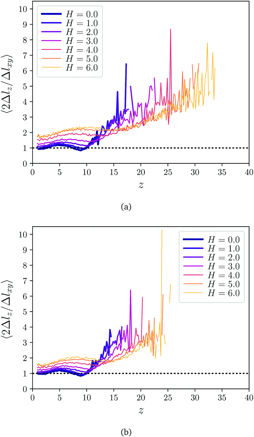Fig. 11 Vertical distribution of average vertical 〈δl_z〉 over horizontal 〈δl_xy〉 elastic deformations of springs calculated for each value of applied magnetic filed. (a) Profiles obtained for ρ = 0.2, K_soft. (b) Profiles obtained for ρ = 0.2, K_stiff.

3.5 Connection to experiments

The increase of the surface roughness of MAE coatings under applied magnetic fields has been reported experimentally very recently.³³ It has been estimated as ΔR_rms/ΔH = 1 μm/T for a particular PDMS-based MAE filled with 70 wt% of carbonyl iron powder, but it has been mentioned that this value can be increased by optimizing the material composition. Our results can be compared to the experimental ones for the fields, in which the magnetic moments of particles are coaligned with an applied field. As shown above, this is the case for the fields in which spatial rearrangements replace in-place rotations. Our findings indicate that the roughness of less concentrated systems is easier to change with smaller H, thus, for low fields the roughness of the most concentrated sample changes only slightly. However, for higher fields one can observe a crossover: for soft samples at H ∼ 5.5 the roughness of the MAE with ρ = 0.25 crosses its counterpart with ρ = 0.20; the analogous crossing between ρ = 0.30 and ρ = 0.20 can be observed at H ∼ 6. We assume that the maximum value of roughness grows with particle concentration, however higher fields are needed to initiate the surface deformation. Moreover, larger values of the surface roughness can be achieved with softer matrices varying the concentrations. This conclusion is supported by the experimental finding in ref. 32. In particular, it has been shown that the water contact angle measured in a magnetic field grows tremendously with increasing content of plasticiser, i.e., by decreasing the elastic modulus of the polymer matrix. This increase of the surface hydrophobicity is assumed to be caused by the field induced growth of the surface roughness.

One of the ways to understand whether the effects described here are measurable is to estimate the applied fields needed to observe them for a real MAE sample. Let us assume that we are dealing with magnetically hard particles like NdFeBr, for instance, whose saturation magnetisation is ∼800 Gauss. Suppose that, without an applied magnetic field, the thickness of the MAE layer is 200 μm, as in ref. 32. In our simulations, the layer thickness in a field-free case is 10 particle diameters. This suggests that the particle diameter associated with our model is about 20 μm. Such a particle would possess a magnetic moment of approximately 3.3 × 10⁻⁶ emu. If we then estimate the field at which the magnetic energy in our simulations roughly coincides with the Zeeman one (H ∼ 5, in our reduced units), we can find that this field corresponds to approximately 400 Gauss, equivalently 40 μT. This is a rather small field in comparison to the values used in ref. 32. This would be the reason for the absence of full saturation in our simulation results. However, the still strong deformations of the samples we obtained evidence that we have a softer matrix than in such experiments. In conclusion, despite we lack experimental measurements that match the conditions we simulated here, the effects and the characteristic behaviour of our model system seem to be realistic enough to guide future experiments.

4 Conclusions and outlook

In this work we studied the deformation of a magnetic elastomer thin coating under applied magnetic fields using coarse-grained computer simulations.

Our simple model represents the magnetic elastomer as a layer of permanently magnetised particles randomly crosslinked by springs. The bottom part of the layer is absorbed on a flat nonmagnetic substrate, whereas the upper part is a free surface. The crosslinking is performed according to a distance and a maximum coordination criteria, and the springs elastic constants follow a normal distribution within selected ranges. Three different volume fractions of magnetic particles and two ranges of spring rigidities were studied, for a relatively broad range of external field strengths. We performed an exhaustive analysis of various system parameters in order to verify that our model is able to adequately capture the main experimental observations of strong changes in the elastomer free surface, particularly in its roughness, that is responsible for this system to provide a magnetically controlled variation of the surface hydrophobicity.

The advantage of our simple model is that it provides an insight into the microscopic nature of the aforementioned effect. It turns out that, in absence of an applied magnetic field, and due to the finite thickness of the sample, the dipolar forces lead to the formation of chains predominantly oriented parallel to the substrate plane. Such a chain formation, however, does not lead to any anisotropy of the elastic stresses. Once an external magnetic field perpendicular to the substrate is applied, the situation changes dramatically. Both, elastic and dipolar forces compete against the Zeeman interaction. The latter tends to align all particles perpendicular to the substrate. As a result of this competition, two regimes of field response are observed for the MAE coating. First, at low fields, magnetic particles tend to mainly rotate in place, avoiding large translational displacements and, thus, without large elastic deformations. This leads to a decrease of the Zeeman energy and to an increase of the dipolar one. By increasing the field one can observe a transition to a different mechanism of structural rearrangement, as the particles start forming chains perpendicular to the substrate. This results in very strong elastic deformations, especially near the free surface of the coating.

The presence of the free surface also leads to an unusual magnetic response of MAE coatings. The magnetic susceptibility becomes a nonmonotonic function of the applied magnetic field, showing a maximum whose position depends on the magnetic particle concentration and matrix rigidity, but, in any case, corresponds to the field strength at which dipolar and Zeeman energies approximately coincide.

The roughness of the surface monotonically grows with the applied magnetic field, and it reaches higher values for soft MAEs. Interestingly enough, we observe a nonmonotonic dependence of the surface roughness on the magnetic particle concentration. This dependence comes from the fact that the surface roughness grows with both, the height of the vertical chains formed by the magnetic particles under strong fields and with the lateral separation between them. If the volume fraction of magnetic particles is low, the formation of vertical chains of magnetic particles at high fields requires very large translational rearrangements that are hindered by elastic constraints, so that formed chains are relatively short and few. If, instead, the magnetic content is very high, translations of particles are hindered by excluded volume interactions, so that the ordering of the particles into long vertical chains is also difficult. Therefore, we have shown that there may exist compositions for the MAE coating that can maximise the roughness of the surface at finite high fields: such optimal composition would be a very soft polymer matrix with a particular magnetic filler concentration.

The discussion presented here suggests that all properties we investigated and, in particular, the surface roughness of MAE coatings, will drastically depend on the thickness of the sample. Our next step is to analyse this dependence, as we foresee the existence of an optimal combination of polymer matrix rigidity, magnetic content concentration, applied field and thickness at which the roughness, and therefore the hydrophobicity of the coating surface, can be maximised. Additionally, we plan to investigate MAE coatings filled with magnetically soft particles. The change in particle magnetic properties will result in a different initial response of the system and a distinct low field balance between dipolar, elastic and Zeeman interactions. For high fields, however, no significant changes are expected, as the same structure of chains aligned with the field will be obtained for magnetisable particles.

Conflicts of interest

There are no conflicts to declare.

Acknowledgements

Financial support of the Russian Foundation for Basic Research is gratefully acknowledged (grant no. 16-29-05276). The authors acknowledge support from the Ministry of Education and Science of the Russian Federation, Contract 02.A03.21.0006 (Project 3.1438.2017/4.6). P. A. S. and S. S. K. are also supported by the FWF START-Projekt Y 627-N27. S. S. K. also acknowledges support from ETN-COLLDENSE (H2020-MSCA-ITN-2014, Grant No. 642774). Computer simulations were carried out at the Vienna Scientific Cluster.

References

1. G. Filipcsei, I. Csetneki, A. Szilágyi and M. Zrínyi, Oligomers – Polymer Composites – Molecular Imprinting, Magnetic Field-Responsive Smart Polymer Composites, Springer, Berlin, Heidelberg, 2007, pp. 137–189.
2. A. M. Menzel, Phys. Rep., 2015, 554, 1–45.
3. S. Odenbach, Arch. Appl. Mech., 2016, 86, 269–279.
4. Y. Li, J. Li, W. Li and H. Du, Smart Mater. Struct., 2014, 23, 123001.
5. Ubaidillah, J. Sutrisno, A. Purwanto and S. A. Mazlan, Adv. Eng. Mater., 2015, 17, 563–597.
6. M. Shamonin and E. Y. Kramarenko, Novel Magnetic Nanostructures, Elsevier, 2018, pp. 221–245.
7. J. de Vicente, D. J. Klingenberg and R. Hidalgo-Alvarez, Soft Matter, 2011, 7, 3701–3710.
8. M. R. Jolly, J. D. Carlson and B. C. Muñoz, Smart Mater. Struct., 1996, 5, 607.
9. C. Bellan and G. Bossis, Int. J. Mod. Phys. B, 2002, 16, 2447–2453.
10. G. V. Stepanov, D. Y. Borin, Y. L. Raikher, P. V. Melenev and N. S. Perov, J. Phys.: Condens. Matter, 2008, 20, 204121.
11. S. Abramchuk, E. Kramarenko, G. Stepanov, L. V. Nikitin, G. Filipcsei, A. R. Khokhlov and M. Zrínyi, Polym. Adv. Technol., 2007, 18, 883–890.
12. G. Stepanov, S. Abramchuk, D. Grishin, L. Nikitin, E. Kramarenko and A. Khokhlov, Polymer, 2007, 48, 488–495.
13. H.-N. An, S. J. Picken and E. Mendes, Soft Matter, 2012, 8, 11995–12001.
14. D. Günther, D. Y. Borin, S. Günther and S. Odenbach, Smart Mater. Struct., 2012, 21, 015005.
15. M. Schümann, D. Y. Borin, S. Huang, G. K. Auernhammer, R. Müller and S. Odenbach, Smart Mater. Struct., 2017, 26, 095018.
16. P. A. Sánchez, T. Gundermann, A. Dobroserdova, S. S. Kantorovich and S. Odenbach, Soft Matter, 2018, 14, 2170–2183.
17. S. S. Abramchuk, D. A. Grishin, E. Y. Kramarenko, G. V. Stepanov and A. R. Khokhlov, Polym. Sci., Ser. A, 2006, 48, 138–145.
18. A. V. Chertovich, G. V. Stepanov, E. Y. Kramarenko and A. R. Khokhlov, Macromol. Mater. Eng., 2010, 295, 336–341.
19. A. Stoll, M. Mayer, G. J. Monkman and M. Shamonin, J. Appl. Polym. Sci., 2014, 131, 39793.
20. V. V. Sorokin, E. Ecker, G. V. Stepanov, M. Shamonin, G. J. Monkman, E. Y. Kramarenko and A. R. Khokhlov, Soft Matter, 2014, 10, 8765–8776.
21. V. V. Sorokin, I. A. Belyaeva, M. Shamonin and E. Y. Kramarenko, Phys. Rev. E, 2017, 95, 062501.
22. I. A. Belyaeva, E. Y. Kramarenko, G. V. Stepanov, V. V. Sorokin, D. Stadler and M. Shamonin, Soft Matter, 2016, 12, 2901–2913.
23. S. Bednarek, J. Magn. Magn. Mater., 2006, 301, 200–207.
24. G. Diguet, E. Beaugnon and J. Cavaillé, J. Magn. Magn. Mater., 2009, 321, 396–401.
25. G. V. Stepanov, E. Y. Kramarenko and D. A. Semerenko, J. Phys.: Conf. Ser., 2013, 412, 012031.
26. A. Zubarev, Physica A, 2013, 392, 4824–4836.
27. A. S. Semisalova, N. S. Perov, G. V. Stepanov, E. Y. Kramarenko and A. R. Khokhlov, Soft Matter, 2013, 9, 11318–11324.
28. I. A. Belyaeva, E. Y. Kramarenko and M. Shamonin, Polymer, 2017, 127, 119–128.
29. I. Bica, Y. D. Liu and H. J. Choi, Colloid Polym. Sci., 2012, 290, 1115–1122.
30. G. V. Stepanov, D. A. Semerenko, A. V. Bakhtiiarov and P. A. Storozhenko, J. Supercond. Novel Magn., 2013, 26, 1055–1059.
31. S. Lee, C. Yim, W. Kim and S. Jeon, ACS Appl. Mater. Interfaces, 2015, 7, 19853–19856.
32. V. V. Sorokin, B. O. Sokolov, G. V. Stepanov and E. Y. Kramarenko, J. Magn. Magn. Mater., 2018, 459, 268–271.
33. G. Glavan, P. Salamon, I. A. Belyaeva, M. Shamonin and I. Drevenšek-Olenik, J. Appl. Polym. Sci., 2018, 135, 46221.
34. M. A. C. Stuart, W. T. S. Huck, J. Genzer, M. Müller, C. Ober, M. Stamm, G. B. Sukhorukov, I. Szleifer, V. V. Tsukruk, M. Urban, F. Winnik, S. Zauscher, I. Luzinov and S. Minko, Nat. Mater., 2010, 9, 101.
35. X. Huang, Y. Sun and S. Soh, Adv. Mater., 2015, 27, 4062–4068.
36. I. Koch, T. Granath, S. Hess, T. Ueltzhöffer, S. Deumel, C. I. Jauregui Caballero, A. Ehresmann, D. Holzinger and K. Mandel, Adv. Opt. Mater., 2018, 6, 1800133.
37. T. Borbáth, S. Günther, D. Y. Borin, T. Gundermann and S. Odenbach, Smart Mater. Struct., 2012, 21, 105018.
38. T. Gundermann and S. Odenbach, Smart Mater. Struct., 2014, 23, 105013.
39. G. Pessot, M. Schümann, T. Gundermann, S. Odenbach, H. Löwen and A. M. Menzel, J. Phys.: Condens. Matter, 2018, 30, 125101.
40. O. V. Stolbov, Y. L. Raikher and M. Balasoiubc, Soft Matter, 2011, 7, 8484–8487.
41. D. Romeis, V. Toshchevikov and M. Saphiannikova, Soft Matter, 2016, 12, 9364–9376.
42. D. Romeis, P. Metsch, M. Kästner and M. Saphiannikova, Phys. Rev. E, 2017, 95, 042501.
43. O. V. Stolbov and Y. L. Raikher, Archive of Applied Mechanics, 2018 DOI:10.1007/s00419-018-1452-0.
44. M. R. Dudek, B. Grabiec and K. W. Wojciechowski, Rev. Adv. Mater. Sci., 2007, 14, 167–173.
45. D. S. Wood and P. J. Camp, Phys. Rev. E: Stat., Nonlinear, Soft Matter Phys., 2011, 83, 011402.
46. D. Ivaneyko, V. P. Toshchevikov, M. Saphiannikova and G. Heinrich, Macromol. Theory Simul., 2011, 20, 411–424.
47. M. A. Annunziata, A. M. Menzel and H. Löwen, J. Chem. Phys., 2013, 138, 204906.
48. G. Pessot, P. Cremer, D. Y. Borin, S. Odenbach, H. Löwen and A. M. Menzel, J. Chem. Phys., 2014, 141, 124904.
49. M. Tarama, P. Cremer, D. Y. Borin, S. Odenbach, H. Löwen and A. M. Menzel, Phys. Rev. E: Stat., Nonlinear, Soft Matter Phys., 2014, 90, 042311.
50. D. Ivaneyko, V. Toshchevikov and M. Saphiannikova, Soft Matter, 2015, 11, 7627–7638.
51. G. Pessot, H. Löwen and A. M. Menzel, J. Chem. Phys., 2016, 145, 104904.
52. R. Weeber, M. Hermes, A. M. Schmidt and C. Holm, J. Phys.: Condens. Matter, 2018, 30, 063002.
53. R. Weeber, S. Kantorovich and C. Holm, Soft Matter, 2012, 8, 9923–9932.
54. R. Weeber, S. Kantorovich and C. Holm, J. Magn. Magn. Mater., 2015, 383, 262–266.
55. A. Ryzhkov, P. Melenev, C. Holm and Y. Raikher, J. Magn. Magn. Mater., 2015, 383, 277–280.
56. A. V. Ryzhkov, P. V. Melenev, M. Balasoiu and Y. L. Raikher, J. Chem. Phys., 2016, 145, 074905.
57. J. D. Weeks, D. Chandler and H. C. Andersen, J. Chem. Phys., 1971, 54, 5237–5247.
58. M. P. Allen and D. J. Tildesley, Computer Simulation of Liquids, Clarendon Press, Oxford, 1st edn, 1987.
59. D. Frenkel and B. Smit, Understanding molecular simulation, Academic Press, 2002.
60. J. J. Cerdà, V. Ballenegger, O. Lenz and C. Holm, J. Chem. Phys., 2008, 129, 234104.
61. A. Bródka, Chem. Phys. Lett., 2004, 400, 62–67.
62. H. J. Limbach, A. Arnold, B. A. Mann and C. Holm, Comput. Phys. Commun., 2006, 174, 704–727.
63. A. Arnold, O. Lenz, S. Kesselheim, R. Weeber, F. Fahrenberger, D. Roehm, P. Košovan and C. Holm, Meshfree Methods for Partial Differential Equations VI, Springer, Berlin, Heidelberg, 2013, vol. 89, pp. 1–23.
64. R. Weeber, S. Kantorovich and C. Holm, J. Chem. Phys., 2015, 143, 154901.
65. J. Schindelin, I. Arganda-Carreras, E. Frise, V. Kaynig, M. Longair, T. Pietzsch, S. Preibisch, C. Rueden, S. Saalfeld, B. Schmid, J.-Y. Tinevez, D. J. White, V. Hartenstein, K. Eliceiri, P. Tomancak and A. Cardona, Nat. Methods, 2012, 9, 676.

---