Comparing the influence of visualization type in an electrochemistry laboratory on the student discourse: who do they talk to and what do they say?

Abstract

A laboratory is a large investment of time and money for departments of chemistry yet discussions continue about its purpose in the educational process. Helping students navigate the three levels of representation; macroscopic, particulate and symbolic is a potential use of this time. This study looked at two different types of visualization for an electrochemistry laboratory in second semester general chemistry and the impact that the visualization type had on the student discourse. Macroscopic visualization (MV) was accomplished through a traditional hands-on laboratory and particulate visualization (PV) was achieved using a computer simulation featuring animated electrons and ions. The type of visualization impacted how much the students talked, who they talked to, and what they talked about. The MV students engaged in less peer-to-peer discussion than the PV students. The MV students expressed more excitement about their observations and were more focused on getting the data quickly. The MV spent most of their time physically doing the laboratory work while spending little time discussing the concepts. The PV students spent more time talking about concepts with their peers especially at the particulate level even answering macroscopic questions with particulate explanations. The type of visualization influenced all aspects of the student discourse.

---

Introduction

Chemistry has always been a learning by doing subject (Pickering, 1993), and the laboratory has been an essential part of the process (Johnstone, 1983) because it allows students to experience phenomena first hand (Hofstein, 2004). Laboratory activities allow students to construct their own understanding of chemistry concepts in a way that lecture or demonstration alone cannot easily accomplish (Bruck and Towns, 2013; Tobin, 1990). However, while the laboratory potentially provides students with opportunities to integrate cognitive, affective and hands-on learning (Galloway et al., 2015), the cost of running a university laboratory can be substantial, and the affect on students’ learning of chemistry remains inconclusive (Hofstein and Lunetta, 1982, 2004; Kirschner and Meester, 1988; Lazarowitz and Tamir, 1994; Lunetta, 1998). Despite this, we still hold on to lab as part of the curriculum because we believe regardless of the type of laboratory practices, it is worth it. The opportunity to visually observe chemical reactions, placing a piece of copper in a colorless solution of silver nitrate and watching the solution gradually turn blue, helps students connect to the chemical concepts (Hofstein, 2004) beyond the written word or the chemical equation. With this in mind, laboratory could still be the ideal place to allow students to engage in meaningful learning while fostering students’ positive attitudes (Lunetta et al., 2007; Galloway et al., 2015).

Learning chemistry is challenging for many students. Its difficulty lies in the complex and abstract nature of the subject (Gabel, 1998; Johnstone, 2000; Tasker, 2014). While students can visually observe chemical phenomena at the macroscopic level (macroscopic view), the explanation of how and why things react as they do lies at the particulate level (particulate view), and usually all of this is summarized and expressed using symbolic representations (symbolic view). Visualization is a key to understanding chemistry concepts and has the potential to lighten the cognitive load for students. Let's take the situation of teaching oxidation–reduction. We define oxidation as the loss of electrons and reduction as the gain of electrons. We might introduce a macroscopic example like rusting to try to tie these definitions to the students’ experiences. Then we jump to the symbolic treatment of oxidation and reduction by writing half reactions and following the loss and gain of electrons through the steps. Chemists are successful in chemistry because they see the connections between these three levels of representational visualization (macroscopic, particulate, and symbolic) and move seamlessly from one to the other (Johnstone, 2000; Talanquer, 2011; Taber, 2013) and therefore do not overload their cognitive processes. Students, novices, treat these three levels of representation as discrete pieces of cognitive material that serve to increase the cognitive load associated with learning chemistry.

There is no doubt, chemists are very interested in the particulate representations of processes, and it is almost impossible to make a connection between the macroscopic level and the particulate level of understanding without some mental image of the way particles interact (Deratzou, 2006). Students do not see this connection and most do not develop it naturally. Since students are sense makers, they do build some type of explanation often creative and inaccurate. Misconceptions found in electrochemistry illustrate this point and are plentiful (Sanger and Greenbowe, 1997, 2000; Ogude and Bradley, 1984; Garnett and Treagust, 1992a). For example, since we cannot see electrons, some students form an image of electrons floating freely in a solution (Ogude and Bradley, 1984) without any assistance from the ions (Sanger and Greenbowe, 1997). Other students imagine electrons moving through a solution by jumping from one ion to the next (Garnett and Treagust, 1992a) or from one electrode to another (Schmidt et al., 2007). Often students see a circuit being completed within a galvanic cell by electrons flowing from one half-cell solution to the other through the salt bridge (Garnett and Treagust, 1992a). An inability to form an accurate image of what electrons are doing at the particulate level not only impedes students’ abilities to acquire the correct conceptual understanding (Songer and Mintzes, 1994; Hamza and Wickman, 2008; Taber, 1995), but also prevents students from integrating the three level of representation during the process of learning (Ogude and Bradley, 1984; Sanger and Greenbowe, 1997). Therefore, if students could visualize an accurate particulate model it would enhance their understanding of the abstract concept (Doymus et al., 2010; Lee and Osman, 2012) and reduce the cognitive load associated with learning chemistry. In the last decade, many chemical educators have taken advantage of freeware programs, using them in both the lecture and in the laboratory to try to assist students in visualizing the particulate level. Computer simulations offer students an explicit view of the interactions at the particulate (sub-microscopic) level (Kozma et al., 2000; Kozma and Russell, 1997; Wu et al., 2001), and are often used as a pre-lab to prepare students for the chemistry laboratory (Winberg and Berg, 2007; Krupnova, 2016), as an alternative to the traditional laboratory for distance learning (Dalgarno et al., 2009; Krupnova, 2016) or as a wholesale replacement of the hands-on laboratory that is much more cost effective (Hawkins and Phelps, 2013; Tatli and Ayas, 2013). Viewing dynamic two or three-dimensional animations has been shown to help students learn to connect the particulate and the symbolic representations (Williamson and Abraham, 1995). Winberg and Berg (2007) found students who used the computer simulation visualization in the pre-lab asked more theoretical questions during the laboratory activity than the traditional group. When comparing achievement on a test following laboratory, students using a computer simulation lab and students in a traditional hands-on lab performed equally well (Hawkins and Phelps, 2013; Tatli and Ayas, 2012, 2013). While there are many studies that compare different laboratory techniques with computer simulations, rarely do these studies emphasize the type of visualization prominent in each type of laboratory and how it affects the dynamics of students’ interactions in the laboratory. In an effort to gain a better understanding of these influences from the students’ perspectives while engaging in an electrochemistry laboratory activity, we deployed two different types of laboratory techniques; a traditional hands-on lab where macroscopic visualization (MV) is prominent, and a computer simulation where particulate visualization (PV) is prominent. We listened to the students’ discourse in hopes of gaining a better understanding of the impact each type of visualization had on students’ learning experiences.

Methods

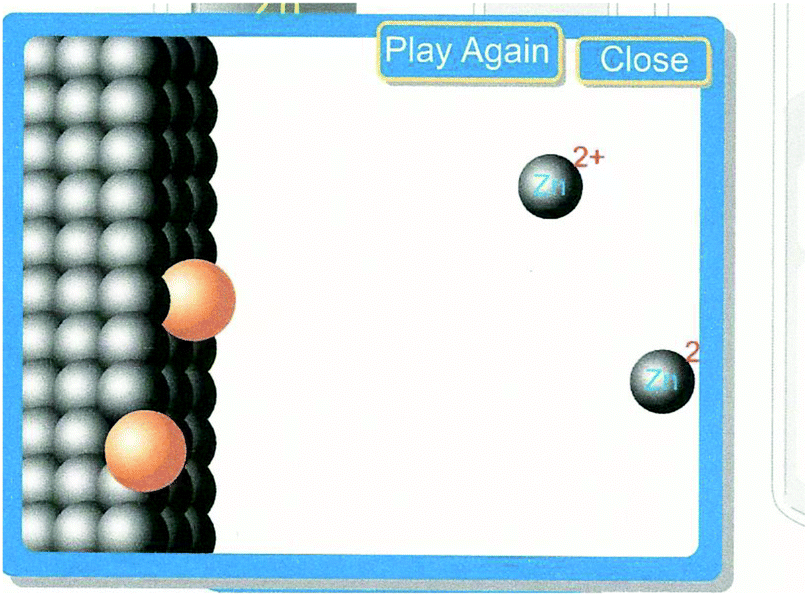
The student discourse data was initially collected from students who were taking the General Chemistry II (CHEM 1121) laboratory at a regional comprehensive university in the Southeastern United States in the Spring semester of 2011. We selected six out of 16 sections of the laboratory to participate in the computer simulation developed by Greenbowe (https://pages.uoregon.edu/tgreenbo/voltaicCellEMF.html) where the visualization was focused on the particulate level laid over an image of an electrochemical cell (see Fig. 1). This selection was based on the availability of the space in the computer lab during the laboratory times. The remainder of the sections performed an electrochemistry experiment using the traditional hands-on approach where the visualization was focused on macroscopic visualizations (MV) such as observing a direct reaction, building galvanic cells, examining the impact of a salt bridge, and measuring voltages with a digital meter (White, 2005). In addition to being enrolled in CHEM 1121, students were enrolled in a General Chemistry II lecture in the semester in which they took this laboratory. Students choose the laboratory section based on a time that was most convenient for them with no regard for the lecture section they are enrolled in. Therefore, students in the simulation laboratories and students in the traditional hands-on laboratories could be in the same lecture sections. The quantitative data obtained from the pre- and post-test was analysed and the results were published in a previous issue of this journal (Hawkins and Phelps, 2013). Permission to use data from human subjects was obtained from our institutional review board (IRB) and informed consent was acquired directly from the students in the laboratory sections. We collected audio recordings from students who provided informed consent from each of the different laboratory techniques as they worked through the material. Six groups of students were recorded; three MV and three PV, four of which were transcribed in the summer of 2015. After we analysed the original data, we found the influence of each type of visualization on the dynamics of student interaction in the laboratory to be interesting, but due to problems we encountered with the quality of the audiotaping, we decided to recollect the student discourse data in the Fall of 2015 and in the Spring of 2016. A new IRB application was made and approved allowing us to continue this study. We selected 18 pairs of students; nine pairs of students from the laboratory sections that participated in the computer simulation particulate visualization activity and 9 others from the sections that participated in the traditional hands-on macroscopic visualization lab. In an effort to focus on the differences in visualization, others factors in the laboratory were made as similar as possible. We wrote similar procedures and questions implementing a Process Oriented Guided Inquiry Learning (POGIL) activity for both of the visualization approaches (http://www.pogil.org). The same professor taught the electrochemistry lab for each section used in the study. The same researcher observed each laboratory section used in the study on the day of the electrochemistry lab. We audiotaped students’ discourse, and videotaped them engaging in the entire electrochemistry activity with consent of the students being recorded. We used qualitative analysis software, ATLAS.ti, to aid with the coding of the data. The audio recordings were transcribed and a grounded theory framework was implemented. The use of grounded theory allowed us to approach the data looking for emergent categories or themes (Urquhart, 2013; Patton, 2015). As the transcripts were read line by line, an open coding system was used to first look for patterns. The initial patterns in this data were ‘type of activity’, ‘who did the students talk to’ and ‘time spent in each activity’. The raw data within these patterns were further coded by two researchers independently and categorized looking for similarities and difference between the two different visualization groups in accordance with the constant comparison technique (Phelps, 1994).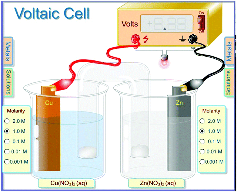

Fig. 1 Screen shot of simulation (used with permission of Dr. Thomas Greenbowe).

Results

The first thing we noticed when comparing the discourse in these two environments was the difference in the total amount of time students spent in the laboratory. The traditional macroscopic visualization (MV) groups spent more time in the laboratory (127 minutes on average) than the simulation particulate visualization (PV) group (89 minutes on average) and the time that they did spend was not spent in the same way.

The data were sorted into categories reflecting the types of discourse that were identified in the transcriptions of the data. Fig. 2 lays out the topics of discourse identified in the data and the percentage of time each group spent engaged in that type of discourse. The two types of discourse that we found most interesting when comparing the two groups were TA/student interaction and peer to peer discussion. MV students spent a greater percentage of their time in lab discussing things with the laboratory instructors, 26% (or an average of 33 minutes), compared to 13% (an average of 17 minutes) for the PV students. PV students spent a greater percentage of their time talking to each other, 66%, compared to 46% for their MV counterparts. Even though this is a greater percentage of time for the PV students it is approximately the same amount of time on average for both groups (just short of 59 minutes). Given the large amount of time both groups spent engaging in peer to peer discussion, this category was further broken down into sub-categories that are displayed in Fig. 3.

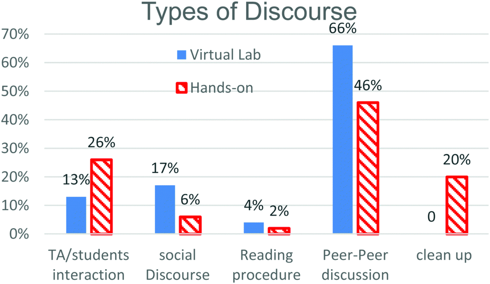Fig. 2 Types of discourse.

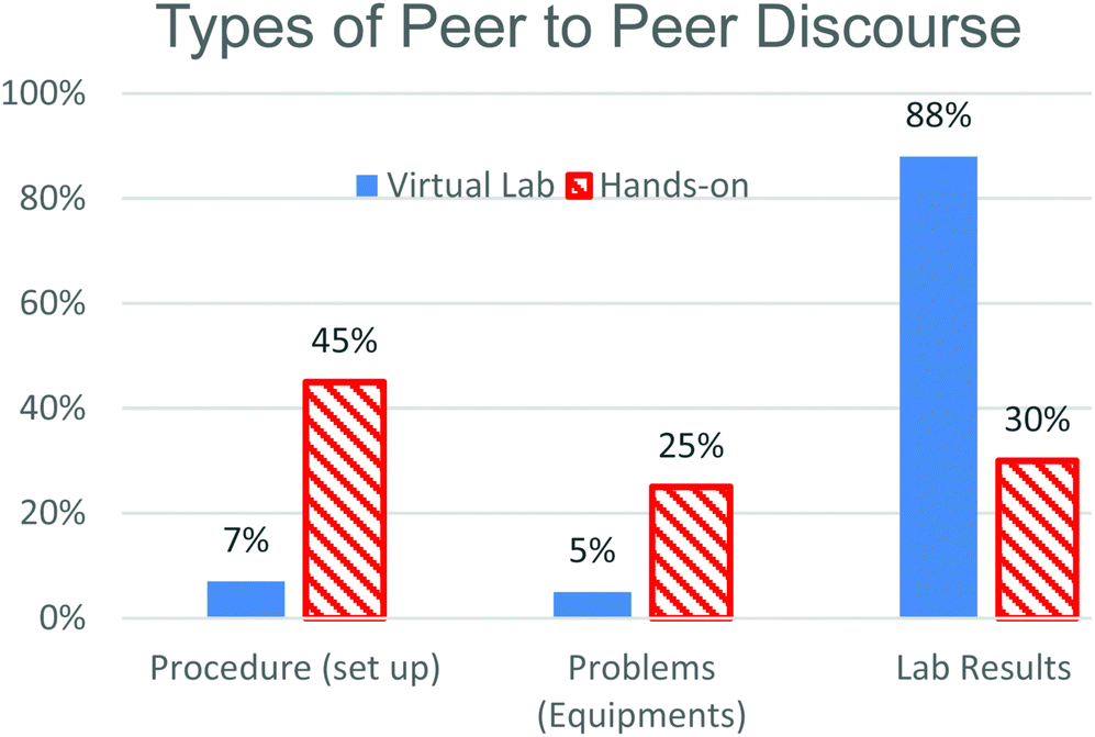Fig. 3 Types of peer to peer discourse.

Three types of peer to peer discourse were identified; procedures, where students were interpreting and setting up the experiment, problems, where students talked about issues with equipment or misunderstandings about how to use equipment, and lab results, which included discussing the data and what it might mean. While the number of minutes spent in peer to peer discussion were similar for the two groups, once you categorized the time into types of discourse, it was interesting that on average PV students spent 52 minutes discussing the results of the experiment compared to 18 minutes for the MV students.

The macroscopic visualization students spent the majority of their peer to peer discussion talking about setting up the experiment and carrying out the laboratory procedures.

MV students:

Jane: I read it and now I forgot… we need a digital multi-meter.

Sally: Multimeter. We also need a Zn strip.

Jane: Is that it?

Sally: It should say on the beaker.

Jane: Yeah, I know, but is that all I’m going to get over here?

Sally: Let's see here, in the second test tube, connect the zinc to one of the wire leads and place the Zn in the test tube… Yes, for now.

Jane: What happened here?

Sally: I don’t know.

Jane: Oh, there we go.

Sally: Does it hook them to here?

Jane: What is this? Did it tell you where you set it (talking about the multimeter)?

Sally: It does not.

MV students:

May: OK… lost it. OK… copper sulphate. Are you watching it?

Peter: Yeah

May: Ok ah…mmm…

Peter: Our test tube is small. Small test tube.

May: Yeah

Peter: That's my mistake.

May: Oh, it's a thing?

Peter. What did you say?

May: Three fourths. (filling test tube ¾ full of solution)

Peter: Three fourths?

May: Yeah. Ok. We’re gonna drop the zinc in. Here we go. Ok drop.

We did code 30% of the MV students’ peer to peer time in the category of lab results, but most of that interaction focused on getting the data with little or no discussion about that data as illustrated by three discussions below.

MV students:

Nancy: It's the right one. Oh my god, it's cool. You get what you get…

Nancy: 1750… 1760 (calling out values on the multimeter)

Drew: 1770… 1784

Nancy: Write it down, do it to it!

Steve: Three… it keeps going up… 300 and we going with 360

Peggy: 360 sound good, Write it down, do it.

Monroe: point 11

Marilyn: point 11?

Monroe: Yeah

Marilyn: Now number 2, or wait… number one without the salt bridge right?

Monroe: That was zero

TA: Stable?

Monroe: Yes

Marilyn: What is it?

Monroe: 1.02

Marilyn: 1.02 ok… so number 3, and now switch the wires connecting the wire lead which had been originally connected to the zinc strip. So switch them again.

Monroe: Umhum… negative 1.02.

The discourse of the students in the macroscopic visualization group was filled with short quips focused on the collection of data both quantitative and qualitative and getting that data collected quickly. There was very little discussion about concepts in the hands-on (MV) lab when compared to the simulation (PV) lab. Not surprisingly, there was very little time spent setting up the experiment for the PV students given the nature of a computer simulation, but a higher percentage of the lab results discourse time was spent interpreting the results.

PV students:

Pepper: When I look at your reactions, and I say to myself which is the most reactive metal? It appears that the zinc metal reacts twice and the silver metal never reacted at all. But here it said the metal (sic) flows from the most reactive to the least reactive. You said silver was the most reactive.

Rey: Umm. The silver's going around just reacting with everything?

Pepper: Good point. Probably not.

Rey: So the difference is silver is plus one and the silver… comes out low metal reactivity when you think about the metal reacting… Looks like your example here. I have two cells for the zinc reactivity, one silver and one copper reactivity.

Pepper: So the zinc, then copper and then silver. Yeah.

Rey: Here, again… electrons getting over here trying to make silver…

Pepper: OK. Zinc, copper, silver. So this is wrong then? And it should be the zinc reacts twice, copper reacts once, silver never reacts?

Rey: How does the activity here of the metal compare to the position (on the table)? OK, now you look at the charge. So, zinc and then the copper and we are backwards. The higher activity is higher on the reaction (table), right?

Pepper: Yeah? OK.

The simulation students spent more time talking about the results of the experiments and the concepts of electrochemistry. More time talking about concepts resulted in PV students revealing more misconceptions. In the previous conversation, for example, the students noticed that silver was the only +1 ion of the substances they were comparing and they want to use this as an explanation for the difference in reactivity. They pointed out silver was the least reactive metal of the triad and the only one with a plus one charge. Although they noticed it, they couldn’t seem to build an explanation that works and eventually dropped the idea. The discussion between the MV students does not reveal as much conflict of ideas because they are focused on getting the numbers, but not explaining them.

It was striking to see how much more conversation about the concept of electrochemistry was happening when students observed the behaviour of electrons at the particulate level. Time was not the only difference in the conversations happening between students in the two groups which becomes more evident when comparing students dealing with similar questions. Let's consider the observation of a direct reaction where students were trying to determine whether copper metal in a zinc sulphate solution or zinc metal in copper II sulphate solution was spontaneous (Fig. 4).

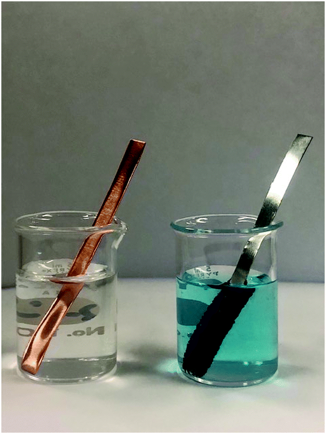Fig. 4 Direct reactions of copper metal in zinc sulphate solution and zinc metal in copper II sulphate solution.

MV students:

Jane: So the metal definitely got darker from silver colour to orangey.

Sally: It got kind of rust coloured.

Jane: It does…

Sally: So observations?

Jane: You can see it looks fuzzy kind of.

Sally: Changing in colour and texture

Jane: Yeah, write that. You got looks orange and rusty

I’m gonna take it out and see what it actually looks like.

Sally: So the texture of the zinc is kind of like fuzzy?

Jane: Yeah, you can see the fuzziness. Do you see it?

Sally: Yeah, I see what you’re talking about.

Jane: Actually it's really cool!

The MV students made macroscopic observations that at times they clearly found exciting. Determining spontaneity for the MV people was about looking for a sign of a chemical reaction.

MV students:

Lillian: Would you say that it's clear?

Adriana: Yeah, royal clear blue.

Lillian: So… royal clear blue.

Adriana: Drop it down… set my timer…

Lillian: I did it… here we go.

Adriana: Whoa… like… immediately.

Lillian: At first I thought that… It kinda like turns black.

Adriana: That's what I'm thinking… but I’m not sure what's black…

Lillian: Throw stuff against the wall… maybe it's displacement?

Adriana: At first… Would you say the solid turned into black or into the zinc?

Lillian: lt kinda looks like…

Adriana: Interesting…

Lillian: Yeah, I think… it (the reaction) is happening… and then…

Adriana: I guess you could say after one minute the zinc is deteriorating.

Lillian: And the copper?

The students reported their observations but did not explore why one reaction occurred and the other did not.

The PV students were also encouraged to set up a direct reaction by placing the copper electrode in the simulation in a solution of zinc nitrate and a zinc electrode in a copper II nitrate solution. The direct reaction was animated for the students at the particulate level (Fig. 5). It would be reasonable to assume that the PV students who could actually see the electrons moving and the ions becoming atoms again would have an easier time determining which reaction was spontaneous.

Fig. 5 Screen shot of animation of a direct reaction (used with permission of Dr. Thomas Greenbowe).

PV students:

Rija: Nothing happens except for this (pointing at the simulation).

Jalon: All the copper went in and zinc out there

Rija: Copper goes in and reacted to zinc

Jalon: So copper attached to the zinc and zinc 2+ releases

Rija: So copper ions go into zinc by taking in the zinc's electrons and they become solid.

Jalon: So that means the…

Rija: It's spontaneous.

Jalon: Yeah.

Rija: Zinc put in copper nitrate so we know zinc started off with zero and then they become a plus two. Copper started out as a plus 2 become zero, so the zinc being oxidized because it's giving up electrons. Which means the copper's being reduced. And the nitrate is just a spectator and there's no reading (on the meter). At this side where copper ions and zinc solid meets that's where reaction is taking place. There's no reading on this.

Jalon: Yeah.

The PV students were trying to answer the same question as the MV students of which reaction was spontaneous, but they talked more about the process than their MV counterparts. While it seems that seeing the electrons moving was helpful to the group above, it wasn’t helpful to everyone.

PV students:

Karen: … I like this visual lab, don’t you?

Richard: Yeah, we don’t have to pour anything out

Karen: Especially the buffer solutions (?)

Richard: Which species loses electrons? That would be copper because it is 2+.

Karen: Ok

Richard: Right.

Karen: And zinc is gained

Richard: Yeah

Karen: The loss of electrons is oxidation. The gain of electrons is reduction.

Richard: This is the half one. Do we need to write that?

Karen: I don’t think so

Richard: OK. So the loss of electrons is oxidation, so the gain is reduction. The zinc is acquiring electrons.

Karen: We are not writing here or just circle?

Richard: Just circle

Karen: The oxidation agent is the zinc and select one… Okay.

These students saw the particulate level animation and they were able to recite the definition of oxidation and reduction, but this did not lead them to the correct interpretation of the reaction.

The question of spontaneity continued as the students moved from observing direct reactions to working with galvanic cells (Fig. 6).

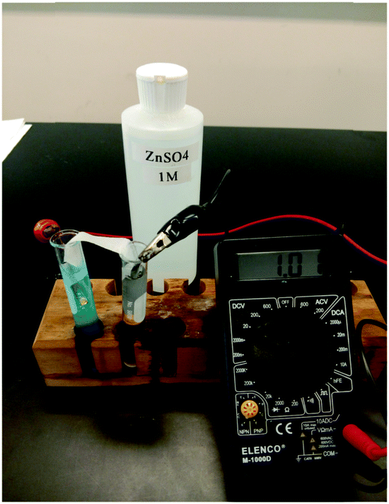Fig. 6 Galvanic cell from MV lab.

MV students:

Sam: These transfers are useful… Is there cell potential (on the meter)?

John: Wow! Do we have electricity!!?

Sam: This is really sick (?). If we have to we can just keep messing with this for the whole lab.

John: Yeah, we do! (answering his own question)

The MV students were still interested in getting readings from the meter and were excited to see that they had created “electricity”. They did not express concerns about determining spontaneity although they were, at times, confused about the sign of the voltage on the meter.

MV students:

Marilyn: What is this? Did it tell you where to set it?

Monroe: It does not.

Marilyn: Get two copper and two zinc.

TA: One copper and one zinc. Did they tell you where to place the copper?

Monroe: Connect a strip of zinc to a wire lead and place the zinc strips in the test tube containing zinc sulphate (Fig. 6).

Monroe: Ok here comes the salt bridge

Marilyn: That went in nice and easy

Monroe: Ok

Marilyn: It's negative, but if we switch it, it will be the same number but positive. So I just have an absolute value of it.

Monroe: Ok, so we take an absolute value of the voltage?

Marilyn: Yeah, if it stops moving… It's gone from 0.08 to 0.3. This is Cu and Fe?

Monroe: Umhum.

Marilyn: Ok… 0.33. Is it capital V or measured in ohms? What's the literature say?

Monroe: I don’t really know.

Most MV groups did not spend much time explaining their results. The peer to peer discourse was much more utilitarian for the MV students. When there were samples of student thinking demonstrated within these MV groups, it was usually initiated by the laboratory instructor (either a graduate teaching assistant or a professor).

MV students:

TA: So which one of these three metals are the most active?

Marilyn; The copper and magnesium.

TA: So you have to name only one.

Marilyn and Monroe: The magnesium.

TA: And the least reactive will be…?

Marilyn and Monroe: The iron.

TA: What's your reason?

Marilyn: Mg is further on the left side of the periodic table so it more easily gives up electrons than iron would.

TA: Can you explain from the data that you obtained from the experiment?

Marilyn: So the Mg easily allows the electrons to be transferred to the copper.

TA: OK but how do you know that?

Monroe: When copper and iron were used, a lot of voltage generated. Anytime Mg was used, the voltage generated was more so…

TA: Very good. In here, you see when Mg and copper… 1.86, right?

Monroe: Yes ma’am

TA: And here you have Mg and Iron at 1.44.

Marilyn: And then just copper and iron then it's only 0.33. And so we can see that there's not a big difference of electrons causing the electrical current.

TA: Why do you say that Mg is the most active?

Marilyn: Because it generates the greatest voltage than any other combination. Anytime magnesium is in there the voltage is much greater.

Monroe: Yes

TA: And you said iron is the least?

Monroe: Yes. It is the same concept. Many times when iron is in there it's less active.

The TA tried to encourage the students to explain their choices for the answers to the questions regarding the reactivity of metals using the data generate by building the various galvanic cells. You can see that the students have the beginning of a concept of activity of metals as it relates to galvanic cells although there are still holes. The idea that a cell containing magnesium will always have the higher voltage works for these three metals, but is not applicable to all cells containing magnesium and they never tied the trend back to relative reduction potentials. Similar conversations happened between the PV students without the prompting by the TA (see Pepper and Rey earlier).

The PV students had a similar galvanic cell set up which included a digital meter much like the one used in the hands on laboratory (Fig. 1). The PV students were able to observe electrons moving through the cell which gave them an advantage when answering questions about a galvanic cell.

PV students:

Mick: Here (in the simulation), you can actually see—you can actually see what's going on.

Mariam: You can also see the copper is sticking to the metal.

Mick: Electrons moving through the wire and then attracting the copper, yes.

Hattie: Yeah, I agree. Plus, oh… first two electrons. Mark the cathode. The anode, I am pretty sure is zinc and the cathode is this (pointing), because that's what she said, yesterday, right?

Daniella: Yes, it (the electron flow) goes from anode to cathode and then from zinc to copper. Cathode is copper?

Hattie: Yes.

Daniella: Anode is zinc.

Hattie: Perfect, so is this still a spontaneous reaction?

Daniella: No, is that where we add at the values and we would do zinc backwards, so it will be positive 0.762. And copper would be the positive, so it's not… it's not spontaneous.

These PV students could see the electrons moving from the anode to the cathode in the animation. They could see how these electrons eventually combined with the cations in the solution of the cathode half-cell (Fig. 1). Despite this information they still had trouble deciding if what they were seeing was a spontaneous reaction even after calculating a positive cell potential. They seemed to confuse the sign convention for cell potential for a product favoured reaction with the sign convention for the change in free energy of a spontaneous reaction.

The calculation of the cell potential was a source of confusion for many students. The calculation of the cell potential is presented in two different ways within our department and in the textbooks in use in our general chemistry courses. One approach is the calculating of the cell potential as the difference in the reduction potential of the cathode and the reduction potential of the anode. The other approach instructs the students to take the sum of the reduction potential of the thing that is reduced (cathode half reaction) and the oxidation potential of the thing that is oxidized (the opposite sign of the reduction potential). The electrochemistry laboratory fell at the beginning of the study of electrochemistry so most students had been introduced to the definitions of oxidation and reduction, but had not engaged in a lot of practice with writing half reactions.

PV students:

Lauren: Which one is the table of…

Anthony: Probably refers to like looking up in here and see which one… Confirming one is bigger than the other one. I’m going to ask her.

Lauren: Ok, zinc

Rezhin: Zinc is point seven six.

Anthony: So, you do need a table as a reference.

Rezhin: Ok, thank you.

Lauren: So zinc has a voltage of negative seven six and silver positive point eight zero. So the difference is 0.04 or point seven six minus point eight zero.

Rezhin: I think zinc is negative point seven six plus point eight zero cause in class today we…

Lauren: We did ah…

Rezhin: But still, I don’t know if it pluses or minuses in general.

Lauren: yeah

Rezhin: I don’t know. I guess we just add them.

Lauren: Point eight minus point three four gives you a point four six (reading the value off the simulation) so that point zero four?

Lauren: So I notice if it's a really small number then…

Rezhin: Yeah so it's smaller than the lowest voltage because I added in point three four (0.34) and point eight oh (.80) and the one point.

Lauren: Or… Ok if that… then we have to compare which one made the smallest (reading on the voltmeter), copper and silver. So copper is point three four (0.34) and silver point eight zero (0.80). Add those together, one point one four (1.14). So I guess the higher the… I don’t know if it's correct. The higher the voltage, the…?

Rezhin: The higher the voltage, the lower the…?

Lauren: The current?

Rezhin: the reduction potential?

Lauren: I think zinc is the most reactive and then copper and then silver.

Rezhin: Yeah

Lauren: Cause zinc is the oxidizer for both copper and silver. Copper is the oxidizer for silver and silver is never the oxidizer.

Rezhin: That makes sense.

Lauren: So how does the activity of the metals compare to their position on the table?

Lauren: Zinc is up here, negative point seven six (−0.76) and both copper and silver are positive. Copper being point three four (0.34); silver point eight (0.8). So the higher the number the less reactive. The anode’ll be the zinc.

These students could see what was happening at the particulate level, but had trouble connecting that to the symbolic representation required to calculate cell potentials from a table of standard reduction potentials. They even seemed confused as to how the values on the standard reduction potentials table were related to the value on the voltmeter in the experiment. They made attempts to apply vocabulary, but confused the idea of things that are oxidized and things that cause other things to be oxidized (reducing agents). It is interesting that while the vocabulary was not accurately applied, the students were able order the metals in terms of reactivity correctly and identify that zinc would be the anode of this triad of elements. The PV students persisted in this type of discussion without intervention from the laboratory instructor.

Students in both the macroscopic visualization lab and the particulate visualization lab were asked to identify which electrode loses mass in the galvanic cell. The macroscopic visualization students responded in a very macroscopic way, simply reporting what they saw.

MV students:

Andrew: It looks like this one is thinner.

Nicholas: Yeah, It looks like it's thinner and maybe lighter?

Andrew: So zinc is getting smaller—will it go away complete?

Nicholas: We only have to say which is smaller.

Initially, the PV students also responded based on what they saw; an electrode getting smaller as electrons travel up the wire and ions leave the anode and enter the solution. The PV students saw which electrode lost mass in the animation, but they tried to explain why this was true.

PV students:

Mick: So the one that loses electrons should be the smaller one.

Ringo: I guess that makes sense losing stuff should make it smaller.

Mick: Ok so losing is smaller.

Ringo: Yeah seems too easy. But…

Mick: Well losing electrons means you have more positive charges than negative so that makes it smaller. That makes sense, right?

Ringo: Sure I guess—so the smaller one is zinc?

Mick: Yeah zinc is smaller and copper is bigger since it gains electrons.

Mick: (laughing) Ok time to get serious, I’m sorry. Ok anyway the one that gets smaller is the one that loses electrons. The one getting bigger is the one that gains electrons.

Ringo: Ooh yeah.

Mick: Because electrons’ repulsion tells us that atoms or ions will get bigger.

Lauren: Each cell in the simulation reacts, which half-cell shows the metals getting smaller?

Raleigh: The smaller?

Lauren: The smaller one would be solid, wouldn’t it? So it would be… because it's the ion that is positive means there's not many electrons out there so it holds it tight together.

Lucy: Which half-cell shows the metal getting smaller?

Ricky: It would be the one that gives away the electrons that will get smaller because it gives away zinc ions… right?

Ricardo: Right? This one's gaining silver ions into it.

Ricky: So cell A, copper is getting smaller.

Ricky: The one that gives off the electrons is smaller because the nuclear pulls from the nucleus.

Despite their good scores on the laboratory assignment, the students revealed some misconceptions as we listened to them that were not evident when merely grading their papers. For example, these students in the particulate visualization group correctly identified the electrode losing mass, but provided well thought out and incorrect particulate level explanations for why they made the choice they made. At times they seemed to equate “pieces of metal” and “metal ions’ since they are both classified as metals on the periodic table. They also used relationships that explained why cations are smaller than their respective neutral atoms to pick the electrode that is “getting smaller” as the electrochemical cell proceeds. The students’ reasoned that losing something should make you smaller but they incorrectly explained this by applying the idea that a loss of electrons causes an increase in the effective nuclear charge which makes the ion radius smaller than the neutral atom radius. Most of the students seemed to ignore that the ions produced by the loss of electrons would be water soluble which would reduce the mass of the anode. This happens despite the fact that the simulation shows cations leaving the anode in one half cell and other cations sticking to the cathode in the other half cell. The students in the macroscopic visualization group also had no trouble choosing correctly the electrode that loses mass. These students just reported the one that looked smaller as smaller without thinking about why that might be true.

Discussion

Assertion: the type of visualization heavily influences the discourse in the laboratory

The type of visualization offered in the laboratory students engaged in impacted who they talked to and what they talked about during the electrochemistry laboratory activity. For students in the traditional hands-on laboratory, the macroscopic view is the critical aspect of the object of their learning and they pay very little attention to the particulate view. They seem to be satisfied with short answers that emphasize colour, texture and meter readings as the important features for completion of the lab. While MV gave students first hand experiences with chemical reactions that, based on their verbal expressions of excitement from the audio tapes of “cool”, and “wow’, engaged them in the activity, the students don’t readily demonstrate that this mode of visualization is leading them to a deeper understanding of electrochemistry concepts. Instead, their discourse focuses on reading and interpreting procedures, and setting up equipment, leaving only 12% of their time in laboratory engaged in peer to peer discussion of the laboratory results. The interactions MV students did have with their peers were generally short, with little or no negotiation of ideas between lab partners and no evidence of making connections to the particulate level of representation. These results, however, do not mean macroscopic visualization has no place in developing conceptual understanding of electrochemistry. The MV students talked more to the instructor in lab and these interactions often led to the development of concepts. The discourse between the TA and students showed that, with careful questioning and guiding from the TA, the students were able to evaluate their data and apply their findings to new situations, and were able to order the reactivity of metals correctly. We want students to be excited about chemistry and develop a macroscopic practical understanding of concepts. For example, the macroscopic visualization was powerful for driving home macroscopic questions, such as which electrode loses mass in a galvanic cell.

The particulate visualization (PV) students talked to each other more than the MV students did and more of that discussion involves interpreting the results of the data collected. Unlike MV groups, where physical phenomena seemed to be the highlight of the experiment, the PV groups, while fascinated with the display of chemical reactions at the particulate level, seemed to focus more on the concepts and interpreting what was happening at the particulate level. While these groups of students provide rich information on how particulate visualization influences how students construct their understanding of electrochemistry, they also reveal various misconceptions. When given these particulate level visualizations, students are cued to try to provide particulate explanations for even macroscopic questions like which electrode gets smaller. PV students consistently carried on involved conversations trying to work out the details to explain phenomena they were observing without prompting from the laboratory instructor. Perhaps due to their relatively low engagement with the laboratory instructors, PV students were not always challenged when they developed alternative explanations that led them to correct answers. This would indicate that the particulate visualization alone is somewhat lacking in helping students develop a complete understanding of chemical processes.

The data in this study demonstrate the strength of the visual phenomenon that students are engaged in when it comes to the type of thinking on display. The activity the students were engaged in heavily influenced the things students talked about. This is important for us to know—it is important for those of us designing laboratories to decide what we want students to get from the laboratory experience and to design accordingly. If we believe that the multiple representations as explained by Johnstone (1983) are important for the learning of chemistry then we need to think about how to use the laboratory to help students make these connections. The laboratory should be a place of excitement where students get a macroscopic sense of chemistry and a WOW factor which was the case for the MV students, but chemistry is also about the particulate understanding since the explanations for most of what students observe at the macroscopic level lie in the particulate level. While both the MV and PV students responded in ways consistent with the primary visualization used in the laboratory they were engaged in, PV students were more likely to explore the “whys” associated with their observations. Both of these results are desirable; excitement about seeing chemistry happen and talking about why chemistry happens that way.

If we want lab to be meaningful (and worth the money and time spent), we have to be more explicit with our objectives and more precise in our design. These data indicate that the type of visualizations we provide the students influences what they think about even when answering the same types of questions. At many institutions the laboratory has remained fairly unchanged for decades, focusing on techniques of data collection and macroscopic observations of chemical phenomena. These types of activities seem to pique the interest of some students and provide a sense of excitement about chemistry. This macroscopic experience is important to the understanding of chemistry, but so is the development of a particulate view of matter. Which begs the question, what would be the impact of combining the two methods? It seems reasonable that combining both the MV and PV approaches into one laboratory experience might help students connect all three levels of understanding; macroscopic, particulate and symbolic. This is in fact what we are doing now and we are excited about this on-going study. There is a large block of time carved out for this laboratory experience and we continue to seek ways to keep the macroscopic benefits while capitalizing on the unused time to enhance particulate understanding as well.

Conflicts of interest

There are no conflicts to declare.

Acknowledgements

The authors would like to acknowledge the help of Dr Gary White who allowed us to work with the students in the CHEM 1120 labs. We would also like to thank Drs Keying Ding and Preston MacDougal for allowing us access to their students. We are also grateful to the students involved in the study who were willing to let us listen in on their conversations.

Notes and references

1. Bruck A. D. and Towns, M., (2013), Development, implementation, and analysis of a national survey of faculty goals for undergraduate chemistry laboratory, J. Chem. Educ., 90(6), 685–693.
2. Dalgarno B., Bishop A. G., Adlong W. and Bedgood D. R., (2009), Effectiveness of a virtual laboratory as a preparatory resource for distance education chemistry students, Comput. Educ., 53, 853–865.
3. Deratzou S., (2006), A qualitative inquiry into the effects of visualization on high school chemistry students' learning process of molecular structure, Doctoral dissertation.
4. Doymus K., Karacop A. and Simsek U., (2010), Effects of jigsaw and animation techniques on students’ understanding of concepts and subjects in electrochemistry, Educ. Technol. Res. Dev., 58, 671–691 DOI:10.1007/s11423-010-9157-2.
5. Gabel D., (1998), The complexity of chemistry and implications for teaching, in Fraser B. J. and Tobin K. G. (ed.), International handbook of science education, Great Britain: Kluwer, pp. 233–248.
6. Galloway K. R., Malakpa Z. and Bretz S. L., (2015), Investigating Affective Experiences in the Undergraduate Chemistry Laboratory: Students’ Perceptions of Control and Responsibility, J. Chem. Educ., 93(2), 227–238.
7. Garnett P. J. and Treagust D. F., (1992a), Conceptual difficulties experienced by senior high school students of electrochemistry: Electric circuits and oxidation reduction equations, J. Res. Sci. Teach., 29, 121–142.
8. Greenbowe, https://pages.uoregon.edu/tgreenbo/voltaicCellEMF.html.
9. Hamza K. M. and Wickman P., (2008), Describing and analyzing learning in action: An empirical study of the importance of misconceptions in learning science, Sci. Educ., 92(1), 141–164.
10. Hawkins I. and Phelps A. J., (2013), Virtual laboratory vs. traditional laboratory: which is more effective for teaching electrochemistry? Chem. Educ. Res. Pract., 14, 516–523.
11. Hofstein A., (2004), The laboratory in chemistry education: thirty years of experience with developments, implementation, and research, Chem. Educ. Res. Pract., 5(3), 247–264.
12. Hofstein A. and Lunetta V. N., (1982), The role of the laboratory in science teaching: Neglected aspects of research, Rev. Educ. Res., 52, 201–217.
13. Hofstein A. and Lunetta V. N., (2004), The laboratory in science education: Foundation for the 21st century, Sci. Educ., 88, 28–54.
14. Johnstone A. H., (1983), Chemical education research facts, findings, and consequences, J. Chem. Educ., 60(11), 968–971.
15. Johnstone A. H., (2000), Teaching of chemistry – logical or psychological? Chem. Educ. Res. Pract., 1(1), 9–15.
16. Kirschner P. A. and Meester M. A. M., (1988), The laboratory in higher science education: Problems, premises and objectives, Higher Educ., 17(1), 81–98.
17. Kozma B. B. and Russell J., (1997), Multimedia and Understanding: Expert and novice responses to different representations of chemical phenomena, J. Res. Sci. Teach., 34(9), 949–968.
18. Kozma R., Chin E., Russell J. and Marx N., (2000), The roles of representations and tools in the chemistry laboratory and their implications for chemistry learning, Journal of the Learning Sciences, 9(2), 105–143.
19. Krupnova T. G., (2016), Interactive virtual laboratory system in teaching and learning chemistry, 3rd International Multidisciplinary Scientific Conference on Social Sciences & Arts Section Education & Educational Research, pp. 517–522.
20. Lazarowitz R. and Tamir P., (1994), Research on using laboratory instruction in science, in Gabel D. L. (ed.), Handbook of research on science teaching and learning, New-York: Macmillan, pp. 94–130.
21. Lee T. T. and Osman K., (2012), Interactive multimedia module with pedagogical agents: Formative evaluation, Int. Educ. Stud., 5(6), 50–64.
22. Lunetta V. N., (1998), The school science laboratory: Historical perspectives and context for contemporary teaching, in Fraser B. and Tobin K. (ed.), International handbook of science education, Dordrecht: Kluwer Academic Publishers, pp. 349–264.
23. Lunetta V. N., Hofstein A. and Clough M., (2007), Learning and teaching in the school science laboratory: an analysis of research, theory, and practice, in Lederman N. and Abel S. (ed.), Handbook of research on science education, Mahwah, NJ: Lawrence Erlbaum, pp. 393–441.
24. Ogude A. N. and Bradley J. D., (1984), Ionic Conduction and Electrical Neutrality in Operating Electrochemical Cells Pre-College and College Student Interpretations, J. Chem. Educ., 71(1), 29–34.
25. Patton M. Q., (2015), Qualitative Research and Evaluation Methods, 4th edn, Los Angeles, CA: SAGE.
26. Phelps A. J., (1994), Qualitative Methodologies in Chemical Education Research, J. Chem. Educ., 71(3), 191–194.
27. Pickering M., (1993), The teaching laboratory through history, J. Chem. Educ., 70(9), 699–700.
28. Sanger M. J. and Greenbowe T. J., (1997), Students’ misconceptions in electrochemistry: Current flow in electrolyte solutions and the salt bridge, J. Chem. Educ., 74(7), 819–823.
29. Sanger M. J. and Greenbowe T. J., (2000), Addressing student misconceptions concerning electronflow in aqueous solutions with instruction including computer animations and conceptual changestrategies, Int. J. Sci. Educ., 22, 521–537.
30. Schmidt H., Marohn A., Harrison A., (2007), Factors that prevent learning in electrochemistry, J. Res. Sci. Teach., 44(2), 258–283.
31. Songer C. J. and Mintzes J. J., (1994), Understanding cellular respiration: An analysis of conceptual change in college biology, J. Res. Sci. Teach., 31, 621–637.
32. Taber K. S., (1995), Development of student understanding: A case study of stability and lability in cognitive structure, Res. Sci. Technol. Educ., 13, 89–99.
33. Taber K. S., (2013), Revisiting the chemistry triplet: drawing upon the nature of chemical knowledge and the psychology of learning to inform chemistry education, Chem. Educ. Res. Pract., 14, 156–168.
34. Talanquer V., (2011), Macro, submicro, and symbolic: the many faces of the chemistry “triplet”, Int. J. Sci. Educ., 33(2), 179–195.
35. Tasker R., (2014), Research into practice: Visualising the molecular world for a deep understanding of chemistry, Teach. Sci., 60(2), 16–27.
36. Tatli Z. and Ayas A., (2012), Virtual chemistry laboratory: Effect of constructivist learning environment, Turk. Online J. Distance Educ., 13(1), 183–199, ISSN 1302-6488.
37. Tatli Z. and Ayas A., (2013), Effect of a virtual chemistry laboratory on students’ achievement, Educ. Technol. Soc., 16(1), 159–170.
38. Tobin K. G., (1990), Research on science laboratory activities: In pursuit of better questions and answers to improve learning, Sch. Sci. Math., 90, 403–418.
39. Urquhart C., (2013)., Grounded Theory for Qualitative Research: A Practical Guide, Los Angeles, Calif.; London: SAGE.
40. White G., (2005), CHEM 1120 Laboratory Manual, Dubuque, IA: Kendall Hunt.
41. Williamson V. M. and Abraham M. R., (1995), The effects of computer animation on the particulate mental models of college chemistry students, J. Res. Sci. Teach., 32(5), 521–534.
42. Winberg T. M. and Berg C. A., (2007), Students’ cognitive focus during a chemistry laboratory exercise: Effects of a computer-simulated prelab, J. Res. Sci. Teach., 44(8), 1108–1133.
43. Wu H., Krajcik J. S. and Soloway E., (2001), Promoting understanding of chemical representations: Students’ use of a visualization tool in the classroom, J. Res. Sci. Teach., 38(7), 821–842.

---